Temperature and Precipitation Extremes Under SSP Emission Scenarios with GISS-E2.1 Model

Abstract

Atmospheric warming results in increase in temperatures for the mean, the coldest, and the hottest day of the year, season, or month. Global warming leads to a large increase in the atmospheric water vapor content and to changes in the hydrological cycle, which include an intensification of precipitation extremes. Using the GISS-E2.1 climate model, we present the future changes in the coldest and hottest daily temperatures as well as in extreme precipitation indices (under four main Shared Socioeconomic Pathways (SSPs)). The increase in the wet-day precipitation ranges between 6% and 15% per 1 °C global surface temperature warming. Scaling of the 95th percentile versus the total precipitation showed that the sensitivity for the extreme precipitation to the warming is about 10 times stronger than that for the mean total precipitation. For six precipitation extreme indices (Total Precipitation, R95p, RX5day, R10mm, SDII, and CDD), the histograms of probability density functions become flatter, with reduced peaks and increased spread for the global mean compared to the historical period of 1850–2014. The mean values shift to the right end (toward larger precipitation and intensity). The higher the GHG emission of the SSP scenario, the more significant the increase in the index change. We found an intensification of precipitation over the globe but large uncertainties remained regionally and at different scales, especially for extremes. Over land, there is a strong increase in precipitation for the wettest day in all seasons over the mid and high latitudes of the Northern Hemisphere. There is an enlargement of the drying patterns in the subtropics including over large regions around Mediterranean, southern Africa, and western Eurasia. For the continental averages, the reduction in total precipitation was found for South America, Europe, Africa, and Australia, and there is an increase in total precipitation over North America, Asia, and the continental Russian Arctic. Over the continental Russian Arctic, there is an increase in all precipitation extremes and a consistent decrease in CDD for all SSP scenarios, with the maximum increase of more than 90% for R95p and R10 mm observed under SSP5–8.5.

1. Introduction

Climate change includes not only changes in the mean climate but also an increase in the occurrence and intensity of extreme events such as hot extremes and heavy precipitation events. In some cases, mean precipitation decreases, whereas extreme precipitation increases due to a higher atmospheric moisture content due to an increased water-holding capacity of the atmosphere in a warming climate [1], which is explained by the Clausius–Clapeyron relation. Global climate models (GCMs) are useful tools for investigating the climate response to different forcings and for climate prediction and projection. Anthropogenic emissions have been associated with large changes in the late twentieth century hot extremes in climate models [2] and human activity has been shown to impact drought events [3,4].

The Coupled Model Intercomparison Project (CMIP) has provided a fundamental basis for the study of climate extreme indices and for understanding the future changes of extremes [5,6]. Previous studies have reported that the global mean precipitation change is constrained by the radiative cooling rate of the atmosphere [7,8]. The rate of global precipitation is increasing by 1–3% per +1 °K due to the energetic constraints while the change in water vapor amount is ~7% per +1 °K due to global warming [9]. Such energetic constraints have been applied in studies on regional precipitation changes [10], although large uncertainties remain regionally and at seasonal scales, especially for extremes. The rate of increase of extreme precipitation may be even greater than the increase in moisture because additional latent heating could invigorate convection and further increase rain rates [8,11,12].

Climate models have projected a general intensification of extreme precipitation events during the twenty-first century on continental to global spatial scales [8,13,14,15]. This general large-scale amplification is consistent with observed trends in extreme precipitation [16,17,18]. The simulated enhancement of extreme precipitation can be attributed to the increased water-holding capacity of warmer air [1].

Many studies have established that precipitation and temperature over land are interconnected due to land–atmosphere feedback [19,20]. Due to land–atmosphere interactions, under increasing atmospheric blocking in a relatively stable atmospheric boundary layer during an intensive heatwave period, the increasing water vapor within the atmosphere may cause extreme warming and extreme precipitation on different scales. On regional scales, the changes in extreme precipitation in a warming climate can differ substantially from the global-scale increase [14,21,22]. Regional differences can be partly due to natural variability [13]. The simulated patterns of forced responses to global warming also exhibit regions with little change and even areas with decreased extreme precipitation [14,21]. Different future scenarios indicate that if no adaptation and mitigation measures are taken in a timely manner, the impacts from extreme warming and precipitation might increase. It has been reported that for Europe, the effect of the excess heating will be magnified by factor of five by 2060 [23].

This study is a continuation of the earlier paper by Nazarenko et al. [24] that provided a summary overview of the GISS climate simulations of the 21st century ScenarioMIP experiments. The motivation for this study was to extend the reported results with simulated changes in climate extremes. The main focus of this paper is to provide a summary of projected future changes in the intensity and frequency of temperature and precipitation extremes in response to different magnitudes of anthropogenic forcings in the twenty-first-century ScenarioMIP scenarios. The effects of different warming scenarios for the 21st century on the temperature and precipitation extremes at the global, regional, and continental scales are presented and compared. In Section 2, we present a brief description of the GISS climate model. The global changes for the temperature and precipitation extremes SSP experiments are discussed in Section 3, while the regional changes are presented in Section 4. The discussions and conclusions are presented in Section 5.

2. Model and Experiments

We use GISS-E2.1 version of the NASA Goddard Institute for Space Studies (GISS) climate model with a 2° latitude by 2.5° longitude horizontal resolution and 40 vertical layers, with the model top near the stratopause at 0.1 hPa. A more complete description of GISS-E2.1, including numerous improvements to the physics since CMIP5, is provided in [25,26]. Kelley et al. [25] describes the improvements of the model physics in the GISS climate model in greater detail as well as an evaluation of the seasonal climatology of the atmospheric and coupled models during the satellite period (1979–2014), while Miller et al. [26] describes the drivers and responses over the historical period (1850–2014). We used two different treatments for the atmospheric composition. The first treatment for the atmospheric composition is a version with a Non-INTeractive (NINT) composition. Three-dimensional monthly mean distributions of aerosols and ozone were prescribed from atmosphere-only simulations with the second treatment of the atmospheric composition that include the fully interactive aerosol and chemistry model. The aerosol indirect effect on clouds was included as a simple parameterization for increasing the low cloud cover in response to increasing aerosols [27]. This parameterization was based on an assumed relation between aerosol number concentrations and cloud fraction and tuned to produce a roughly −1.0 W/m² of forcing in 2000 relative to 1850 (see [26] for a discussion). The ocean model is a mass conserving model with a horizontal resolution of 1.25° longitude by 1° latitude and has 40 vertical levels with finer resolution in the top 100 m. The improvements to the physics since CMIP5 for the ocean model were documented in the paper by Kelley et al. [25].

The four different future scenarios from the ScenarioMIP experiments in the CMIP6 [28], which extend the historical simulations from 2015, that are mostly used in this study represent the following simulations: the SSP1–2.6 scenario (sustainability) with lower carbon emission levels, reduced inequality, and an emphasis on reducing anthropogenic emissions, transiting to renewable energy supplies, educational and health investments. SSP2–4.5 (middle of the road) assumes moderate carbon emissions and moderate GDP (Gross Domestic Product) and population growth. SSP3–7.0 (regional rivalry) reflects the path with high air pollutant emissions, expansion of cropland, fast population growth, and little investment in education and health. SSP5–8.5 scenario (fossil-fueled development) consists of a tripling of the greenhouse emissions over the course of the 21st century, rapid population growth, and low adaptability. SSP1–2.6, SSP2–4.5, SSP3–7.0, and SSP5–8.5 represent low, medium, high, and very high GHG emission scenarios, respectively, with radiative forcings of 2.6, 4.5, 7.0 and 8.5 W m⁻² in 2100 [29]. For the analysis of the future changes in the global mean values, we also discuss the results for future projections for other SSP scenarios.

In addition to discussing the changes in temperature and precipitation extremes for the geographical maps, we evaluated the projections of extremes over each continent and averaged the extremes of six continents (excluding Antarctica): Asia (excluding Russian Arctic), Europe, Africa, Australia (Aust), North America (NAm), and Central and South America (CSAm). In addition, the Russian Arctic region (RAR) was considered separately to demonstrate the different changes in the extremes in this region. In this study, we considered a subset of 8 indices for temperature and precipitation following the Expert Team on Climate Change Detection and Indices (ETCCDI) [30,31]: the daily minimum (TNn) and maximum (TXx) temperatures, the total wet-day precipitation, the 95th percentile threshold of the wet-day precipitation (>1 mm) (R95p), the maximum 5-day precipitation accumulation (RX5day), heavy precipitation days (>10 mm, R10 mm), the simple daily intensity index (SDII), and consecutive dry days (CDD). More detailed information on these indices can be found on the ETCCDI website (http://etccdi.pacificclimate.org/indices.shtml, accessed on 1 January 2025). These selected indices give an overview of the projected changes in major temperature and precipitation extremes. Most indices are presented on an annual basis, although a few are also shown as seasonal changes.

3. Global Changes

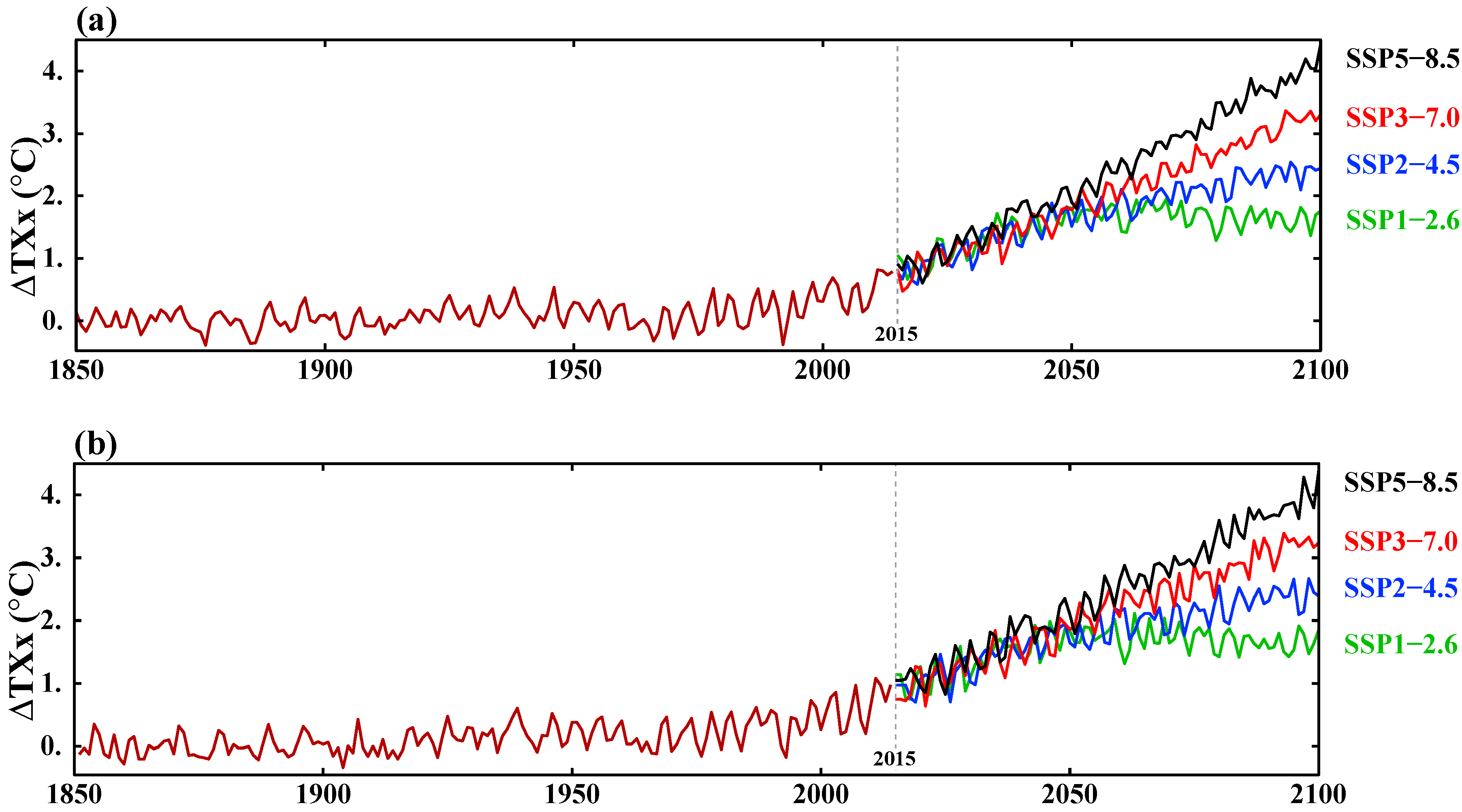
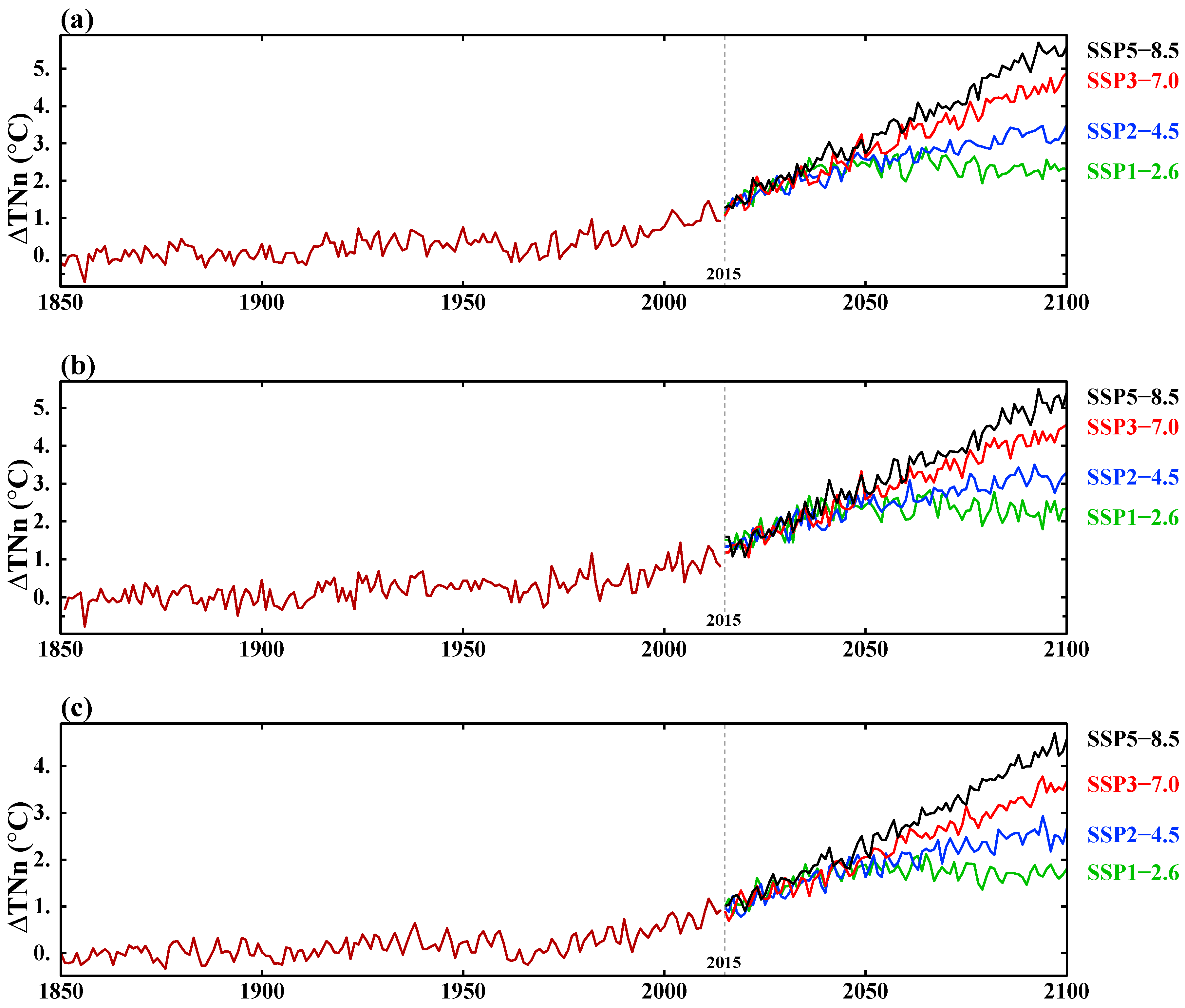
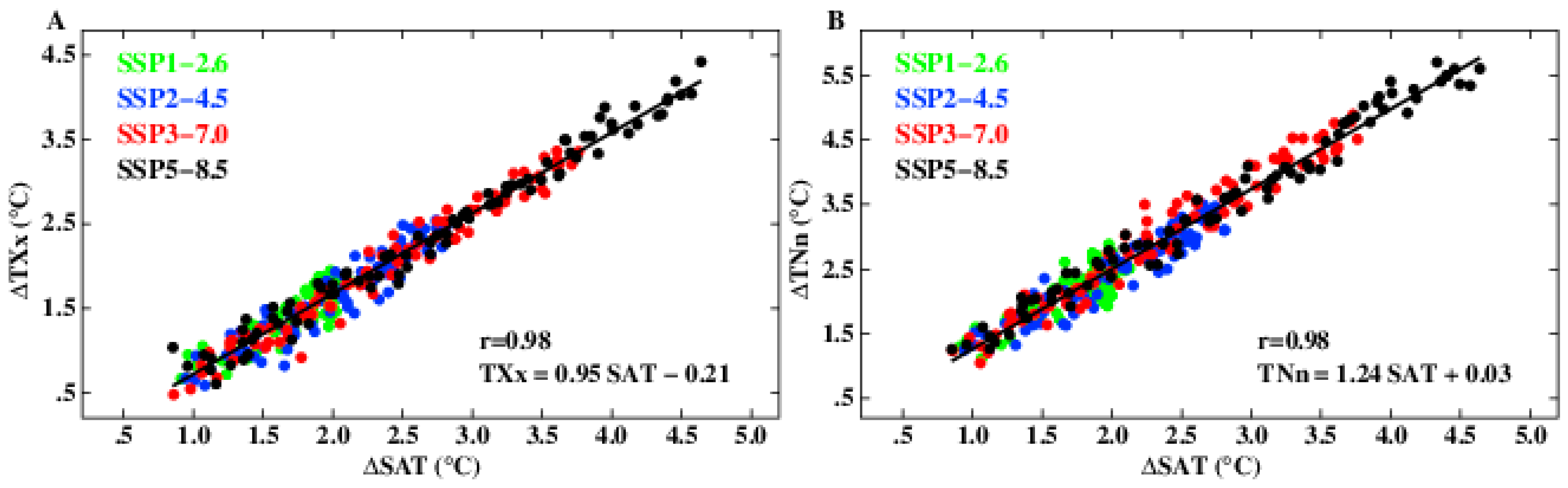
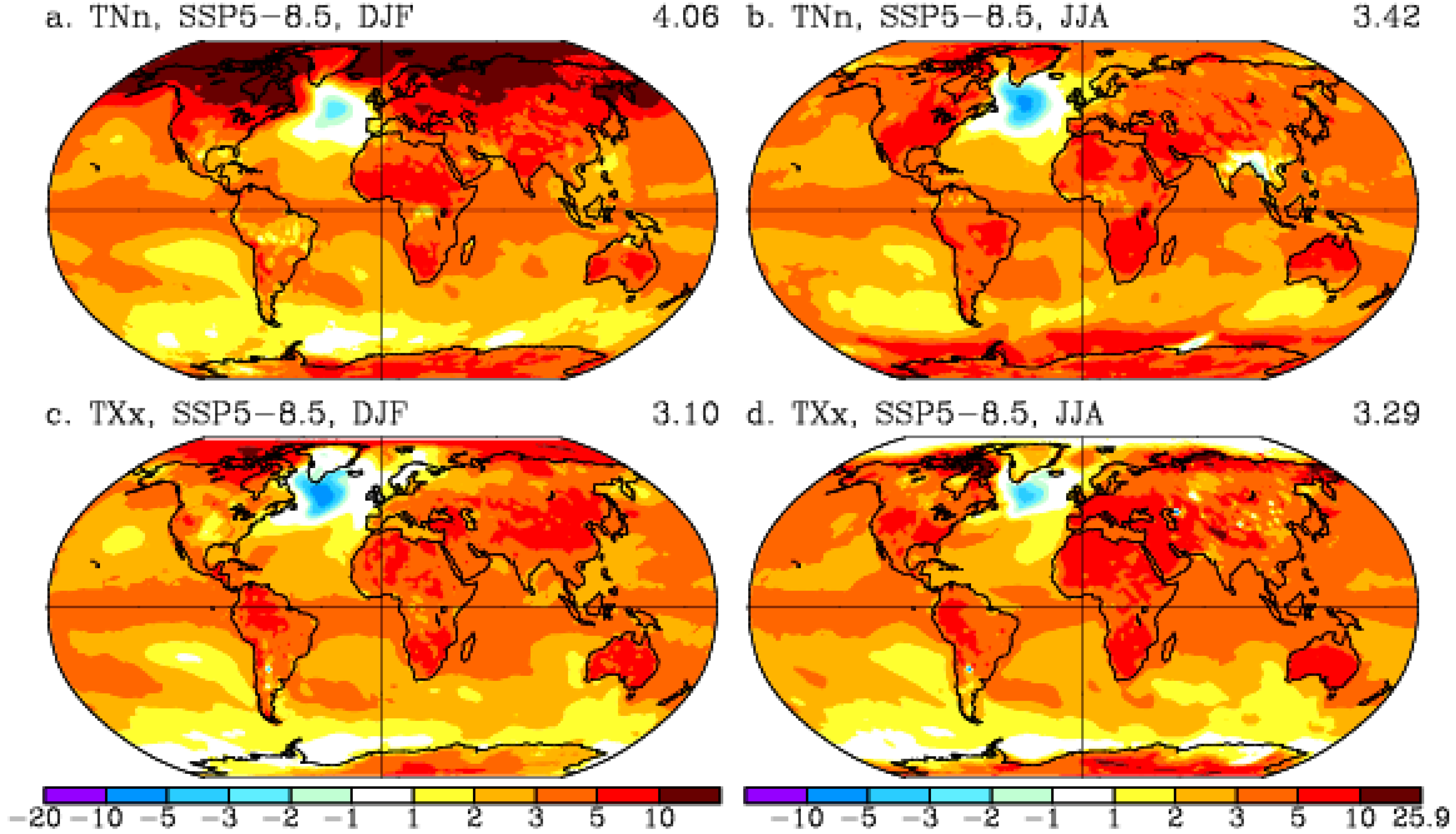
3.1. Temperature Extremes

The days with the minimum (TNn) and maximum (TXx) temperatures represent the coldest and hottest day of the year, season, or month, respectively. Relative to the 1850–1900 reference period, there is a general increase in both minimum and maximum global surface temperatures for the annual, DJF, and JJA means (Figure 1 and Figure 2). The increase in TNn is greater than for TXx for all the scenarios, which is shown in Supplementary Figure S1 in the same plot. TNn is shown as solid lines and TXx is shown as dashed lines.

It was noted earlier that the warming over land is greater than over ice-free ocean areas [32]. Over the northern 30–90° N land areas, the increases in both temperatures are greater (Supplementary Tables S1 and S2) than the global mean temperature warming for the annual, winter, and summer averages. Supplementary Figures S2 and S3 show the maximum and minimum temperatures for the northern 30–90° N land areas and the global means in one plot where the stronger warming over northern land can be seen. The solid lines show the northern 30–90° N land area temperatures, the dashed lines show the global mean temperatures.

The increases in global mean temperatures ranged between 1.5 °C and 4.4 °C, and between 1.5 °C and 5.6 °C for TXx and TNn, respectively (Figure 1 and Figure 2). Over the northern 30–90° N land areas, the increase in the range of temperature in 2100 was found to be between +0.7 °C and 5.4 °C and between +4.0 °C and +9.6 °C for TXx and TNn, respectively (Supplementary Tables S1 and S2; Supplementary Figures S2 and S3).

The increase in the coldest temperature (TNn) over the Northern Hemisphere land areas is stronger (up to 3 times for some scenarios and in some seasons) than the increase in hottest temperatures (TXx) (Supplementary Tables S1 and S2). This stronger warming of the coldest temperatures was also reported by Sillmann et al. [30] for CMIP5 RCP2.6, RCP4.5, and RCP8.5 over the Northern Hemisphere land areas. While the coldest temperature (TNn) warming is quite unform for all seasons, the increase in the hottest temperatures (TXx) is much greater over winter than over summer. In the latest IPCC assessment [33], the projected warming is greatest in the higher latitudes, particularly in the Northern Hemisphere, and greater in the low-sun season than the high-sun season.

For the low GHG emission scenarios SSP1–1.9 and SSP1–2.6, there is a gradual decrease in both TXx and TNn after 2050 for all seasons (Supplementary Tables S1 and S2). The special scenario SSP5–3.4 OS also showed a decrease in temperatures, especially for the coldest temperatures (TNn) (Supplementary Table S2). This shows the achievement of the goal of reducing the greenhouse forcing in scenario SSP5–8.5 from the middle of the 21st century to the values of scenario SSP4–3.4. For the global mean temperatures, the degree of warming is very close for scenarios SSP4–3.4 and SSP5–3.4 OS at 2100. Over the northern land areas, the reduction in warming is stronger for the coldest temperatures in SSP5–3.4 than in SSP4–3.4 (Supplementary Table S2). The stronger warming of the hottest temperatures in SSP5–3.4 OS compared to SSP4–3.4 is due to large inertia of strong forcings in the daytime temperatures over the land areas (Supplementary Table S1).

The projected rates of change in the hottest (ΔTXx) and coldest (ΔTNn) daily temperatures relative to warming in the surface air temperature (ΔSAT) are presented in Figure 3. These rates are expressed as linear regressions for the hottest temperature (TXx = 0.95 SAT − 0.21) and for the coldest temperature (TNn = 1.24 SAT + 0.03), respectively. There is strong correlation (r = 0.98) between both the hottest (ΔTXx) and coldest (ΔTNn) daily temperature anomalies and the surface air temperature anomalies (ΔSAT). Generally, increases in temperature extremes outpace warming in global surface air temperature. There is a stronger increase in TNn per 1 °C of global warming (Figure 3B) compared to the TXx increase (Figure 3A). The maximum TNn warming of 5.6 °C and the maximum TXx warming of 4.4 °C versus 4.6 °C global warming is projected in SSP5–8.5. The minimum TNn warming of 1.1 °C is about double the 0.6 °C TXx warming. The rates of TXx and TNn change in the low-emission scenario SSP1–2.6 are smaller than those in the other scenarios.

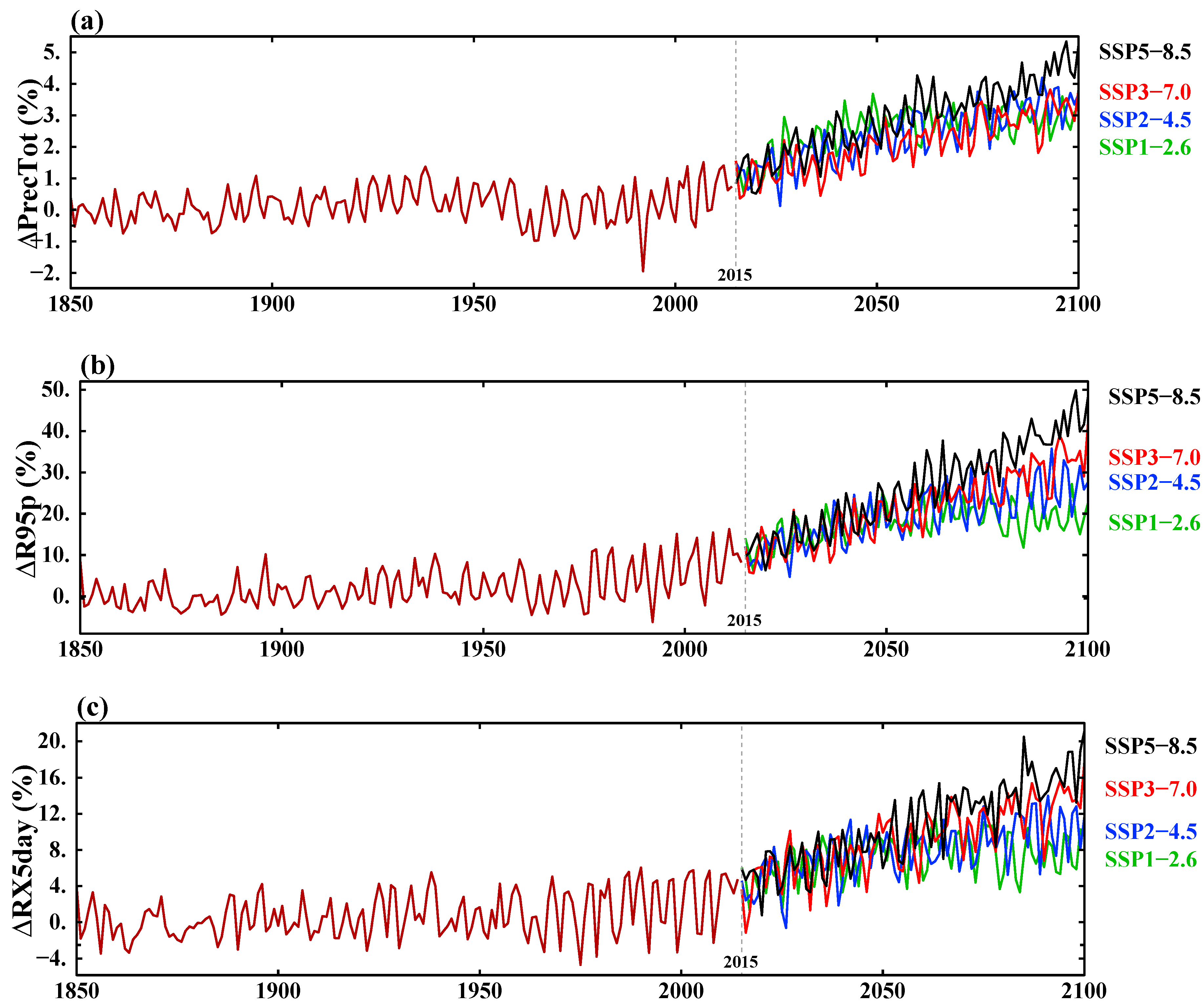
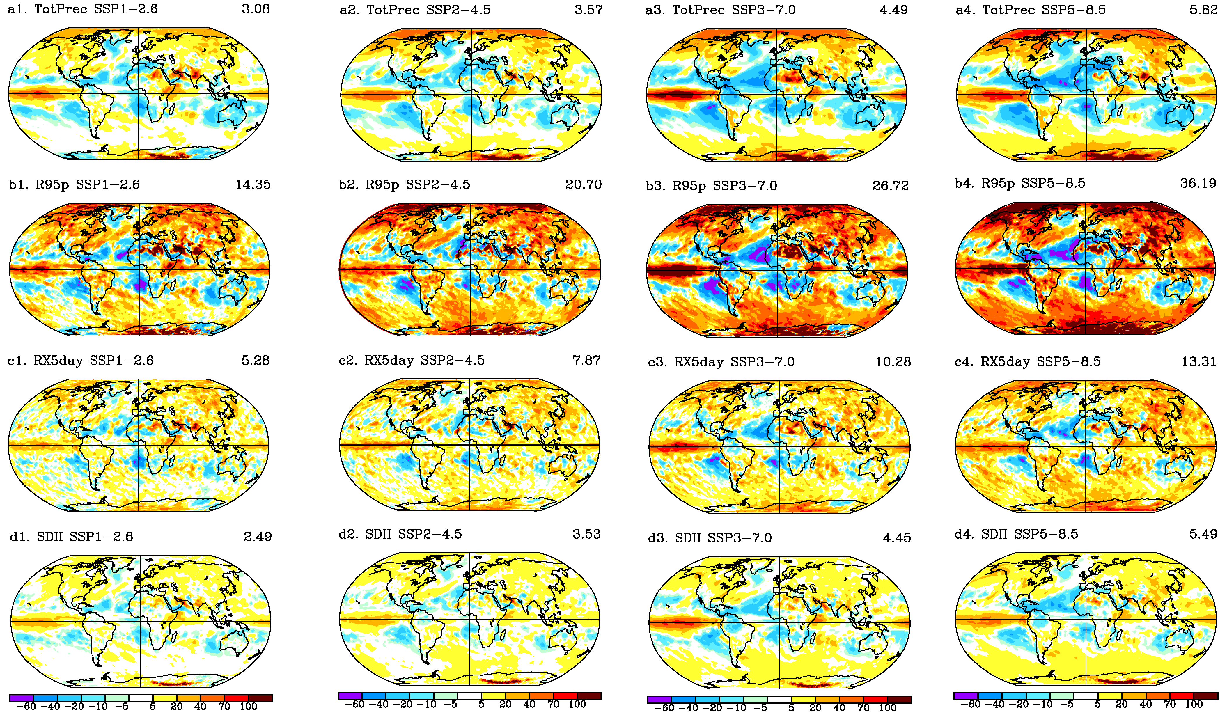
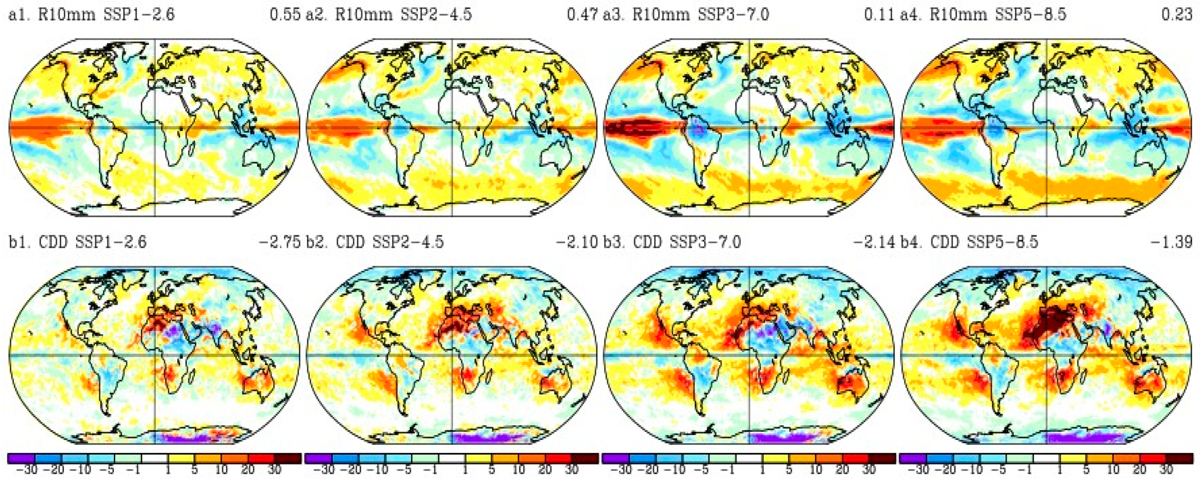
3.2. Precipitation Indices

Changes in the global mean precipitation indices, such as total wet-day precipitation, the 95th percentile threshold of the wet-day precipitation (>1 mm) (R95p), and the maximum 5-day precipitation accumulation (RX5day), relative to the pre-industrial 1850–1900 reference period are shown as percentages in Figure 4. The time evolution of all three indices projected under the four SSP scenarios before 2040 are generally the same. After 2040, the indices begin to show some differences.

Global mean annual mean precipitation must be equal to global mean annual mean evaporation at the surface. Deforestation reduces evaporation and therefore precipitation [34]. Changes in extreme precipitation are not necessarily controlled by a balance between precipitation and evaporation [35]. The effect of different aerosol emissions on the change in total precipitation for the different SSPs was also reported in earlier studies [28,36,37].

The largest increase in total precipitation of 5.2% by year 2100 was found for SSP5–8.5 while an increase of 3.2% was found for the low-GHG emission scenario SSP1–2.6 (Figure 4a). At the end of the 21st century, the increases in total precipitation are similar for SSP1–2.6, SSP2–4.5, and SSP3–7.0 (Figure 4a), although the total warming in SSP3–7.0 is +7 W/m² by the year 2100 [24]. This warming is much stronger and should have a larger effect on precipitation compared with the +2.6 W/m² and +4.5 W/m² values in the warming scenarios. In addition to warming, SSP3–7.0 is a special scenario with large aerosol emissions that apparently have a stronger effect on precipitation changes compared with the usual precipitation increase due to warming. The rapid decreases in aerosol emissions due to aggressive reductions in fossil fuel consumption cause larger increases in total precipitation in SSP2–4.5 and SSP1–2.6 due to warming than in SSP3–7.0. The larger aerosol emissions in SSP3–7.0 (due to weak pollution control policies) would cause smaller increases in total precipitation than in the other SSP runs. Greater negative responses of total precipitation to larger aerosol emissions compensate for the positive responses of total precipitation to the GHG forcing in SSP3–7.0. The business-as-usual scenario SSP5–8.5 with the largest warming (+8.5 W/m²), primarily due to GHG forcing, has the largest increase in total precipitation (+5.2%). The total forcing in SSP5–8.5 is larger than in SSP3–7.0, so the general GHG warming is more overwhelming in SSP5–8.5.

Regarding heavy rain conditions, both the maximum 5-day precipitation and the 95th percentile of the wet-day precipitation show increases consistent with those of total precipitation (Figure 4b,c). An almost 50% increase in heavy precipitation (Figure 4b) and 20% increase in consecutive 5-day heavy precipitation (Figure 4c) are projected for SSP5–8.5, which also reflect the larger capacity of the warmer air to accumulate and hold moisture in this scenario.

The global mean precipitation averages demonstrate that extreme rainfall increases at a faster rate by the year 2100 compared to the total precipitation. Figure 5A shows a scaling of the 95th percentile of the wet-day precipitation (ΔR95p) versus the surface temperature (ΔSAT) (R95p = 9.47 SAT + 0.05). The large correlation of r = 0.89 confirms the direct effect of global warming on the acceleration of the worsening heavy rain conditions. The increase in the wet-day precipitation ranges between 6% and 15% per 1 °C of global surface temperature warming. Figure 5B demonstrates a scaling of the 95th percentile (ΔR95p) versus the total precipitation (ΔTotPrec) (R95p = 8.07 TotPrec + 1.34), with very strong correlation (r = 0.9). This shows that the sensitivity of extreme precipitation to warming is about 10 times stronger than that of the mean total precipitation.

Supplementary Figure S4 demonstrates the changes in total precipitation and 95th percentile of the wet-day precipitation for the northern 30–90° N land areas and the global means in one plot. The solid lines show the northern 30–90° N land area temperatures, and the dashed lines show the global mean temperatures. Consistent with stronger warming over land (Supplementary Figures S2 and S3; Supplementary Tables S1 and S2) than over the entire globe, the increases in total wet-day precipitation are larger over the northern 30–90° N land areas than the global mean (Supplementary Figure S4a). For SSP5–8.5, the increase by 2100 is about three times larger. The heavy precipitations over the northern land areas are about three times larger than the total precipitation change (Supplementary Table S3). For the warmest scenario SSP5–8.5, the 95th percentile of the wet-day precipitation is about 4 times higher over the northern 30–90° N land areas compared to the global mean increases in 2100 (Supplementary Figure S4b).

For the low GHG emission scenarios SSP1–1.9 and SSP1–2.6, there are decreases in total precipitation after 2050 (Supplementary Table S3), which indicate a cooling of temperatures (Supplementary Tables S1 and S2). The same trend for precipitation and temperatures after 2050 was also noted for the special scenario SSP5–3.4 OS. The partial decreases in the heavy rain conditions and in the maximum of 5-day precipitation accumulations were also noted in 2100 for both SSP1–1.9 and SSP1–2.6, as well as for SSP5–3.4 OS (Supplementary Tables S3 and S4) due to reductions in warming and cooling relative to the middle 21st century.

Supplementary Table S4 shows the annual and seasonal changes for the 30–90° N land maximum 5-day precipitation (RX5day) relative to the 1850–1900 base period. Annually, RX5day increases in all the SSPs. The largest increase of 20% was observed under SSP5–8.5. The maximum 5-day precipitation changes in 2100 are stronger in DJF than in JJA over the northern land for most of the SSP scenarios (Supplementary Table S4). This reflects stronger warming in DJF for both the hottest (Supplementary Table S1) and coldest (Supplementary Table S2) days.

The simple daily intensity index (SDII) is a climate index that measures the average amount of rainfall on rainy days (days with at least 1 mm of precipitation) over a specified period. It is calculated by dividing the total precipitation on wet days by the number of wet days. A higher SDII indicates more intense rainfall on wet days. This index for the northern 30–90° N land areas shows increases, with the largest increase of 11.7% in SSP5–8.5 (Supplementary Table S3). The increases in SDII are in line with the increases in total precipitation as well as with the wet-day precipitation indices R95p and heavy precipitation days (>10 mm, R10mm). The number of the consecutive dry days (CDD) in the Northern Hemisphere land areas consistently decreases, although the changes in CDD are not uniform over continents. The regional changes are discussed in the next section.

Probability density functions (PDFs) are often used to illustrate how climate variables change in variability, skewness, or shape of the distribution in the future relative to the present [38]. Figure 6 shows the estimated PDFs of the extreme precipitation index (1850–1900) anomalies for the global mean for four SSPs and historical experiments. For all six precipitation extreme indices, the histograms become flatter, with reduced peaks and increased spread, compared to the historical period of 1850–2014. The mean values shift to the right end (toward larger precipitation and intensity). The higher the GHG emissions of the SSP scenario, the more significant the change in the index.

4. Regional Changes

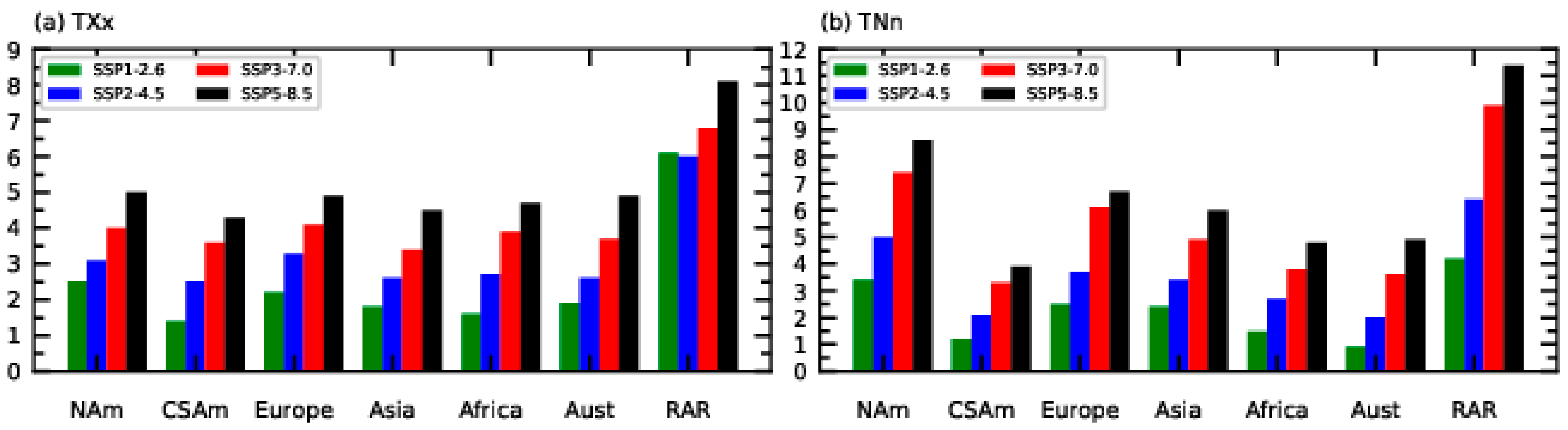
4.1. Temperature Extremes

The geographical distributions of the annual minimum and maximum temperature changes for the last twenty years of the twenty-first century (2081–2100) relative to the last twenty years (1995–2014) of the corresponding historical simulation are shown in Figure 7 and Figure 8 for four selected scenarios: SSP1–2.6, SSP2–4.5, SSP4–7.0, and SSP5–8.5. The numbers in the upper right corner are the global mean values. The same color bar is applied to each column of the maps in Figure 7 and Figure 8, e.g., Figure 7a (Figure 8a) uses the color bar of Figure 7c (Figure 8c) and Figure 7b (Figure 8b) uses the color bar of Figure 7d (Figure 8d). The smallest spatial variability was observed under SSP1–2.6 and the largest variability was observed under the high-emission scenario SSP5–8.5. The spatial patterns of the changes in TNn (Figure 7) and TXx (Figure 8) are different. In particular, TNn increases more strongly in higher latitudes in the Northern Hemisphere. It was reported that the minimum temperatures in northern Europe have warmed the fastest over the last few decades, consistent with the expected influence of greenhouse warming [39,40,41]. For the low-emission scenario SSP1–2.6, TXx only moderately changes over land (Figure 8a), while TNn increases by 2–3 times (Figure 7a), particularly in northern latitudes.

The greatest changes in TNn, between 10 °C and 15 °C, were found in SSP5–8.5 in regions such as North America, Northern Europe, and Northern Asia, with the maximum warming being about +24 °C over the high latitudes in the North Atlantic (Figure 7d). The stronger increase in TNn over the high latitudes is related to the retreating snow and ice covers under warming scenarios that is a further continuation of the warming trend in the Arctic region that has been observed over recent decades [42]. Since the sea ice decrease is much larger for the high-emission scenarios SSP3–7.0 and SSP5–8.5, the increase in TNn over the Arctic and high northern latitudes is about a 2-fold larger (Figure 7c,d) compared to the moderate GHG emission scenario SSP2–4.5 (Figure 7b). In the tropics, the TNn increases are comparable with the increases in TXx.

The largest increase in TXx was found to be over the continents, such as over South and North America, northern and central Eurasia, as well as over Africa and Australia. Even in the low-emission scenario SSP1–2.6, there is a substantial increase in TXx over the Mediterranean region and adjacent parts of Europe and Central Europe, Northern Africa, and the Arabian Peninsula (Figure 8a). The projected patterns of TXx changes are consistent among all the future scenarios, and also with the results of the CMIP5 analysis by [43]. More intense increases in TXx over the continents is clearly seen for scenarios with a stronger forcing: SSP2–4.5 (Figure 8b), SSP3–7.0 (Figure 8c), and SSP5–8.5 (Figure 8d).

The seasonal increases in TNn and TXx are presented in Figure 9 for the highest GHG emission scenario SSP5–8.5. The strong Arctic and high northern latitude increase in TNn (Figure 9a) is generally more pronounced in DJF (with maximum warming of about +24 °C) whereas warming in JJA is more homogeneous over all continents (with maximum warming of about +11 °C) (Figure 9b). The general wintertime warming trend in Europe and high northern latitudes is well established [44]. In contrast to TNn, the increases in TXx are stronger in JJA (Figure 9d) than in DJF (Figure 9c), with the largest increase of about +26 °C over high northern latitude land regions. The increase in TXx in DJF is about +11 °C over the Arctic and high latitude land regions (Figure 9c).

Similar patterns of seasonal and regional changes in TNn and TXx are seen in all the other SSP scenarios, although they are less pronounced in the low-emission scenarios SSP1–1.9 and SSP1–2.6 compared to SSP5–8.5 (Supplementary Tables S1 and S2 for global DJF and JJA means). However, even in the lowest forcing scenario SSP1–1.9, the increase in TNn in DJF is more than +5 °C over high northern latitudes.

The spatial variations projected for TXx and TNn over seven continental land areas (NAm—North America; CSAm—Central and South America; Europe; Asia; Aust—Australia; RAR—Russian Arctic Region) are shown in Figure 10a,b and Supplementary Table S5. The temperature changes are presented for the last twenty years (2081–2100) relative to the 1995–2014 reference period. The increase in TXx is quite uniform for all continents except for the Russian Arctic region, which shows the greatest warming (+6.1 °C, +6.0 °C, +6.8 °C, and +8.1 °C for SSP1–2.6, SSP2–4.5, SSP4–7.0, and SSP5–8.5, respectively) for all scenarios compared to all the other continental areas (Figure 10a). Differences in regional warming are clearly seen in the TNn changes, with stronger warming over the higher latitudes, the Russian Arctic (+4.2 °C, +6.4 °C, +9.9 °C, and +11.4 °C for SSP1–2.6, SSP2–4.5, SSP4–7.0, and SSP5–8.5, respectively), and North America (+3.4 °C, +5.0 °C, +7.4 °C, and +8.6 °C for SSP1–2.6, SSP2–4.5, SSP4–7.0, and SSP5–8.5, respectively) (Figure 10b). Europe and Asia show the second strongest warming after the high latitude regions. There is a smaller increase in TNn over the continents with large tropical coverage (Central and South America, Africa, and Australia) compared to the higher latitudes (Supplementary Table S5).

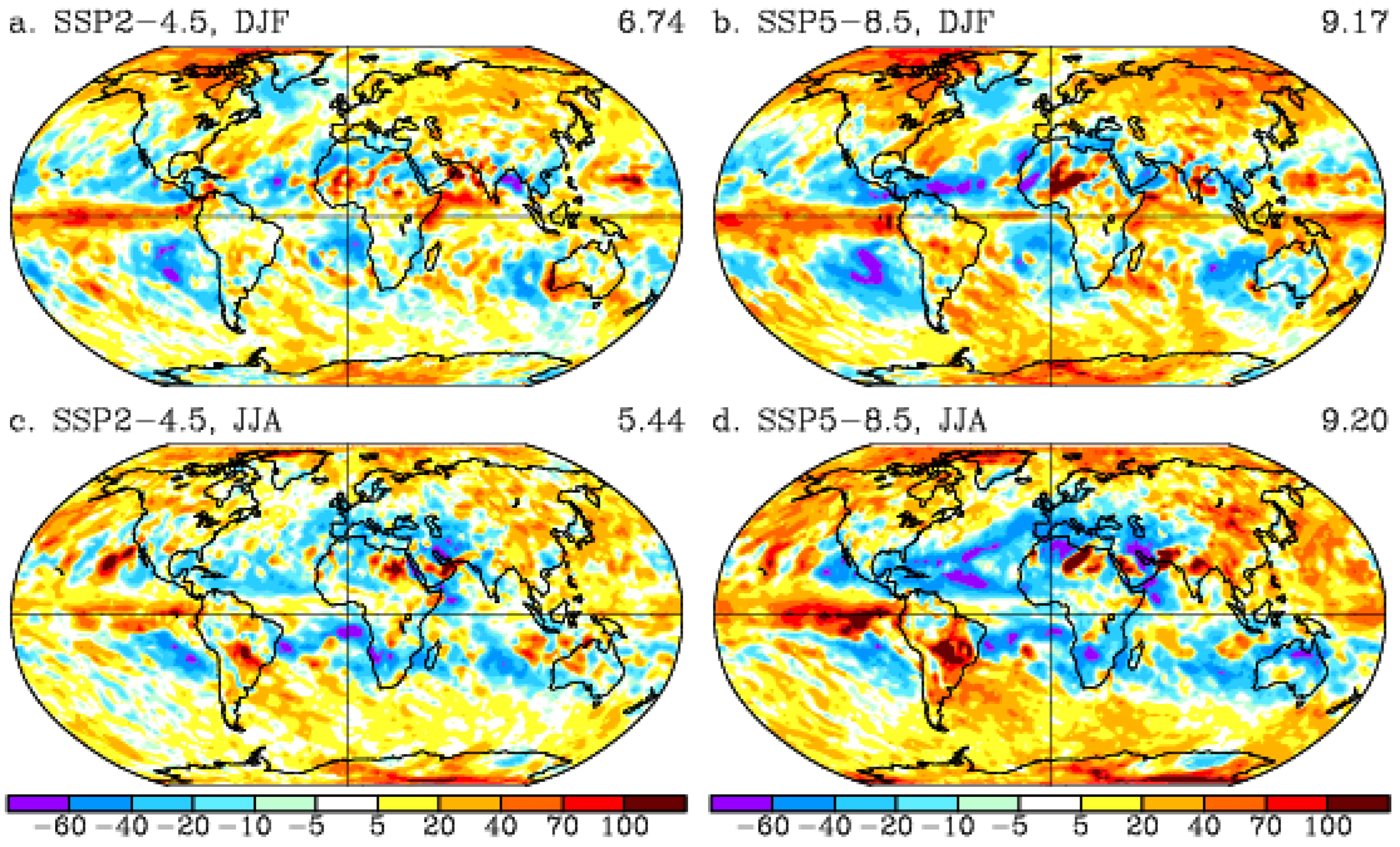
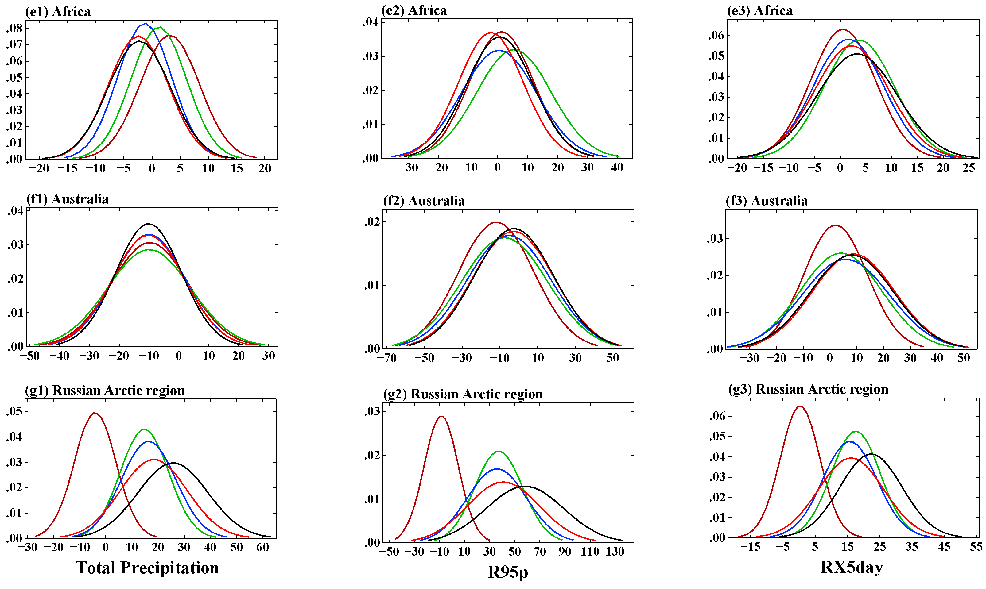
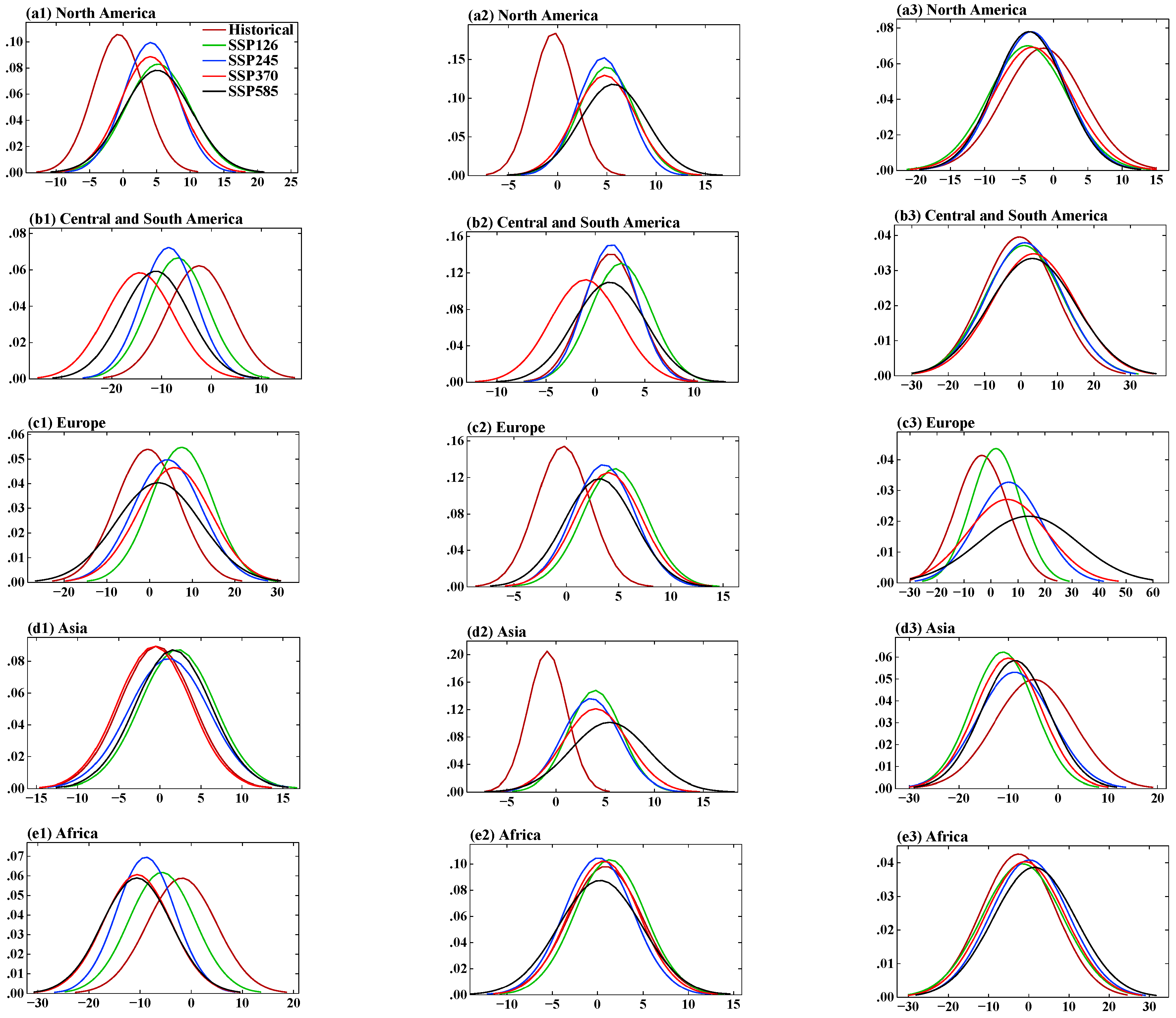
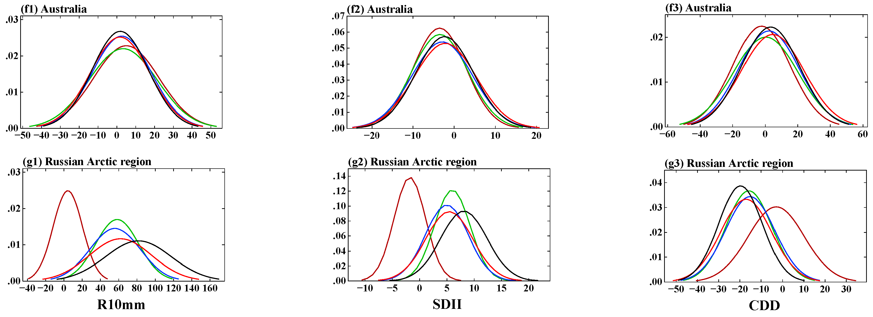
4.2. Precipitation Extremes

The spatial patterns of extreme precipitation are shown in Figure 11, Figure 12 and Figure 13. By the end of the 21st century, there is an increase in total wet-day precipitation over large parts of the Northern Hemisphere continents, Arctic Ocean, east Africa, south of Southern America, the Southern Ocean, as well as Antarctica and the intertropical convergence zone in the Pacific Ocean relative to the 1995–2014 reference period (Figure 11(a1–a4)). Over the continents, the largest changes are projected to be over northeastern Eurasia and the northern part of North America. The higher the emissions of the SSP scenario, the more significant the increase, with the maximum increase found under SSP5–8.5 in the northeast of Eurasia, with an increase reaching more than 50% higher than that of the base period (Figure 11(a4)). Areas with projected decreases in total precipitation include Australia, South Africa, the Mediterranean region, Central America, and sub-tropical ocean regions.

The regional changes in total precipitation generally coincide with the changes in the 95th percentile of the wet-day precipitation (Figure 11(b1–b4)) and the consecutive 5-day heavy precipitation (Figure 11(c1–c4)). R95p increases in high northern and southern latitudes and over the most regions of the northern continents, including more than 70% of the northeast of Eurasia, in SSP5–8.5 (Figure 11(b4)). R95p decreases in Central America, South Africa, and the Mediterranean, with a more than 50% reduction relative to the base period (Figure 11(b1–b4)). The contribution of very wet days (Figure 11(a1–a4)) to the annual total precipitation (Figure 11(b1–b4)) generally shows stronger increases in all SSPs, similar to the results for the global mean quantities (Figure 5B). The regional decreases in R95p are larger compared to the reductions in total precipitation.

Regionally, the greatest increase in RX5day was found for high northern and southern latitudes and the inter-tropical convergence zone in the Pacific Ocean for both annual (Figure 11(c1–c4)) and seasonal (Figure 12) changes relative to simulated late historical (1995–2014) period. Over the high northern latitude regions, the increase in RX5day is less pronounced in JJA, with an increase of 40–70% (Figure 12c,d) compared an increase of more than 70% in DJF (Figure 12a,b). The opposite changes are seen over Southeast Asia, where the summer increases in RX5day are larger than the winter increases. Over the Mediterranean region, such as the south-west European regions and Northern Africa, there are large RX5day decreases in summer (Figure 12c,d) and small increases in winter (Figure 12a,b).

Regions in the Southern Hemisphere, such as Australia and south Africa, experience large decreases in RX5day in winter (JJA) (Figure 12c,d). In Central America, the annual RX5day decreases (Figure 11(c1–c4)) as well as the seasonal response (Figure 12). The decrease in RX5day in combination with the projected increase in CDD suggests severe drying of these regions in future climate projections.

The regional changes in the simple daily intensity index (SDII) as a daily precipitation amount greater than 1 mm a day are shown in Figure 11(d1–d4). The regional changes in SDII coincide with the changes in total precipitation (Figure 11(a1–a4)) as well as R95p (Figure 11(b1–b4)). The projected SDII index shows an increase in most parts of the world, with the regions showing the most significant increase being northern and eastern Eurasia, northern North America, and Northern Africa, which have an SDII reaching more than 20–30% under the high-emission scenarios (Figure 11(d3,d4)).

The regional decreases in both total precipitation and R95p are generally accompanied by a significant increase in the maximum number of consecutive dry days (CDD), as shown in Figure 13(b1–b4). In particular, significant increases in CDD occur in Central America, northeastern South America, the Mediterranean region, Southern Africa, and western Eurasia while CDD decreases in the northeastern Eurasian continent and northern North America compared with the base period. The higher the emissions of the SSP scenario, the more significant the CDD index changes. On the contrary, in South and Southeast Asia, the increases in CDD (Figure 13(b1–b4)) are combined with increases in both R10mm (Figure 13(a1–a4)) and annual mean RX5day (Figure 11(c1–c4)), especially summer (JJA) RX5day (Figure 12c,d), resulting in an intensification of both wet and dry seasons in these regions. The projection of heavy precipitation days (>10 mm) also increases, most significantly over the northern continental regions. Similar to the total precipitation, the higher the emissions of the SSP scenario, the larger the predicted increase in heavy precipitation (Figure 13(a1–a4)).

The continental average extreme precipitation indices are summarized in Supplementary Table S5 and Figure 14 as the 2081–2100 changes relative to the 1995–2014 period. For the continental averages, reductions in total precipitation were found for South America, Europe, Africa, and Australia, and increases in total precipitation were found for North America, Asia, and the continental Russian Arctic (Supplementary Table S5). For the low-emission scenario SSP1–2.6, there is a small increase in total precipitation over South America, Europe, and Africa that could be explained by the flattening of the warming trend over the second half of the 21st century (Figure 1 and Figure 2). Over the continental Russian Arctic, there is an increase in all precipitation extremes and a consistent decrease in CDD for all SSP scenarios, with a maximum increase of more than 90% for R95p and R10mm under SSP5–8.5 (Supplementary Table S5; Figure 14b or Figure 14e).

A summary of the consecutive 5-day heavy precipitation changes relative to the 1995-2014 base period over seven continental land areas are shown in Figure 14c and Supplementary Table S5. The results indicate significant intensification of extreme precipitation, with warming over all continental regions. The largest increase of 27% was found for the Russian Arctic region under SSP5-8.5, and even a small decrease of 0.6% was observed over Africa under SSP3-7.0. This demonstrates the uneven changes in heavy precipitation over different regions and continents under strong warming scenarios. The continental means for the higher latitude regions (North America, Asia, Australia, and Russian Arctic) show larger increases in heavy precipitation while Africa, Europe, and South America experience less extreme precipitation under all the warming scenarios.

It is noteworthy that the R95p (Figure 14b), RX5day (Figure 14c), and SDII (Figure 14d) extremes over Europe and Asia increase while the CDD index is also projected to increase, although the change in CDD over Asia is different under different SSP scenarios (Figure 14f). In general, the future CDD index for North and South America, Asia, and Africa has greater uncertainty, with some area showing increases and decreases under different SSP scenarios (Supplementary Table S5; Figure 14f). This indicates that different regions of the continents experience both wet and dry conditions under different warming scenarios. In Africa, there is high variability in the lengths of long dry conditions that span many years and increased warming. The non-uniform continental change in CDD is more pronounced with stronger warming. These findings indicate that precipitation becomes more uneven in space and time. Moreover, as the emissions in the SSP scenario increase, the uneven distribution of precipitation becomes more pronounced. This non-uniform response to global warming was also reported by [14] for temperature and precipitation extremes in the CMIP5 ensemble.

Figure 15 and Figure 16 present the estimated probability density distributions of the mean annual continental extreme precipitation anomalies (relative to the 1995–2014 climate conditions) for the historical and four SSP scenarios. As was noted before, the different continents experience significant regional variations in extreme precipitation. For North America, the PDFs for total precipitation (Figure 15(a1)) and for all the heavy precipitation indices (R95p—Figure 15(a2); RX5day—Figure 15(a3); R10mm—Figure 16(a1); SDII—Figure 16(a2)) widen, implying a larger area with reduced peaks and increased spread than expected compared to the historical experiment, indicating more precipitation and a stronger intensity. Consistent with the heavy precipitation indices, the PDF for the consecutive dry index is shifted to the left for all SSPs compared to the historical experiment over North America (Figure 16(a3)). The peak of CDD increases for the high-emission scenarios SSP3–7.0 and SSP5–8.5, which confirms the larger variability in CDD under strong warming.

For Central and South America, the uneven changes in the different precipitation indices are very pronounced. While the PDFs for the total precipitation and R10mm are shifted to the left and have more variabilities under the different SSPs (Figure 15(b1); Figure 16(b1)), the PDFs for R95p and RX5day are shifted to the right (Figure 15(b2,b3)), demonstrating increases and smaller variabilities. Uneven changes in the PDFs of SDII were confirmed for stronger warming scenarios (Figure 16(b2)). The slight shifts in the PDFs for CDD in all SSP scenarios (Figure 16(b3)) show an intensification of dry conditions in Central and South America along with stronger heavy precipitation (such as R95p and RX5day).

While the PDFs over Europe did not show changes in the total precipitation in the different SSP scenarios (Figure 15(c1)), there is an intensification of all the extreme precipitation indices (R95p—Figure 15(c2); RX5day—Figure 15(c3); R10mm—Figure 16(c1); SDII—Figure 16(c2)) as well as an increase in drought conditions (CDD—Figure 16(c3)). This demonstrates that both floods and drought periods are possible under warming in the different SSP scenarios. Non-uniform regional changes, such as droughts in the south and floods in the north, were reported for extreme precipitation over China in earlier studies [45,46,47,48,49].

The analysis of the PDF indices for Asia confirmed that the non-uniform response for different regions of continents under different SSPs, such as intensification of total precipitation and heavy precipitation (Figure 15(d1–d3); Figure 16(d1,d2)) as well as reductions in droughts, although there are larger variabilities in CDD changes under the SSPs (Figure 16(d3)). These uneven changes in CDD over Asia under the different warming scenarios is shown in Figure 14f (maps shown in Figure 13(b1–b4)). The average over the entire continent Asia is not very informative since there are sub-regions that experience severe desert droughts, with monsoon rainy seasons, with floods in the south and droughts in the north parts of eastern China. This leads to the canceling out or minimization of the extreme precipitation changes after calculating the continental mean for Asia. It could be worth considering the changes over sub-regions in Asia in a future project. These results align with those of a prior study that found significant increases in precipitation extremes under the SSP5–8.5 and SSP2–4.5 scenarios [50]. In particular, it was noted that there were non-linear changes in the hydrological cycle, which affected precipitation patterns.

There are changes in all the precipitation extremes over the high northern latitudes and the Russian Arctic region (Figure 15(g1–g3); Figure 16(g1,g2)) and there is a consistent decrease in consecutive dry days (Figure 16(g3)). The increase of precipitation over high latitudes in the Northern Hemisphere was reported in the study by [51], with the largest precipitation increase observed in SSP5–8.5. All the extreme precipitation indices show consistent large increases in precipitation over the Russian Arctic region in stronger warming scenarios (Supplementary Table S5).

The PDFs widen implying a larger area (a larger standard deviations) than expected, based on internal variability, experiencing more precipitation, stronger intensities, and longer dry spells by the end of 21st century.

5. Discussion and Conclusions

We described the extreme temperature and precipitation responses to forcing for the CMIP6 SSP future scenarios (2015–2100) using the GISS-E2.1 climate model. In this study, we mostly investigated four scenarios: SSP1–2.6, SSP2–4.5, SSP3–7.0, and SSP5–8.5, although we also discussed the results for other SSP future scenarios.

Increases in both maximum and minimum temperature extremes outpace the warming of the global surface air temperature by a factor of 4–5. Consistent with the CMIP5 RCP2.6, RCP4.5, and RCP8.5 results reported by [30], there is stronger warming of the coldest daily temperatures compared to the hottest daily temperatures. This larger increase in the coldest temperatures than the warmest temperatures implies that the diurnal temperature range may be narrower. Two high-mitigation scenarios, SSP1–1.9 and SSP1–2.6, which were designed to maintain the surface warming below 2 °C [52] at the end of the 21st century relative to the pre-industrial surface temperature, showed a gradual decrease in both TXx and TNn after 2050 for all seasons compared to strong warming scenarios SSP4–7.0 and SSP5–8.5. This suggests that the emission reduction plans can have a substantial effect on mitigating the warming of temperature extremes.

Regardless of the choice of the forcing scenario, there are large-scale features of the temperature extremes, such as stronger warming over land than over ice-free ocean areas, polar amplification, and more rapid warming in cold extremes than in hot extremes. The hot extremes show regional exceptions compared to the cold extremes. The scenario projections show somewhat stronger warming over tropical and subtropical land and ocean areas in hot extremes compared to the cold extremes.

The results indicate an intensification of patterns of change in extreme temperatures with increasing radiative forcing for the future scenarios of the 21st century. Both temperature extremes show small spatial variability for the low-emission scenario, SSP1–2.6, although the warming over the high northern latitudes is 2–3 times stronger for the coldest daily temperatures compared to the mid-latitudes and tropics, reflecting the polar amplification effect. The largest warming of the daily minimum temperatures is over North America, Northern Europe, and Northern Asia. The warming of the daily maximum temperatures is uniform for different continent areas.

The changes in the seasonal minima of TNn are more pronounced in northern regions where the warming is stronger in winter compared to summer. Strong temperature increases in high northern latitudes have been associated with different mechanisms, including reductions in winter ice and snow cover, indirect responses to decreases in summer ice cover, and increased summer ocean heating, as well as increased surface heat fluxes [53]. The continental tropical regions, such as Central and South America, Africa, and Australia, show less winter warming. In contrast, changes in the seasonal maxima of TXx are more uniformly distributed the land globally.

The projected results show that compared with the total precipitation, the mean global extreme precipitation significantly increases in all future scenarios, with most obvious and largest increases observed in SSP5–8.5, confirming the direct effect of strong warming on accelerating increases in heavy precipitation. The sensitivity of the 95th percentile of the wet-day precipitation is about 10 times stronger than the sensitivity of the mean total precipitation versus surface temperature.

Compared with the historical period, precipitation extremes are projected to intensify over the most regions of the world, with the most obvious increase in northeastern Eurasia and the northern part of North America. The stronger the warming in the SSP scenario, the more significant and more intense the increase in precipitation extremes. The increases in total precipitation over the northern land areas are larger than the global mean increases, which is consistent with the stronger warming over land than over the entire globe. Stronger winter warming compared to summer warming over northern land is reflected by larger increases in extreme precipitation and RX5day, particularly during winter months. These pattern changes are broadly comparable to those of the CMIP5 models [14,30].

The results presented here show the reversal or slowing of increasing precipitation extremes for the low-emission scenarios SSP1–1.9 and SSP1–2.6, as well as in the special scenario SSP5–3.4 OS (Supplementary Table S3), in response to stabilizing and cooling global temperatures in 2100. Although the precipitation recovery is slow and delayed, it highlights that the precipitation projections under reduced and stabilized warming can substantially deviate or reverse to some extent the precipitation changes observed under strong warming scenarios, like SSP3–7.0 and SSP5–8.5. The delayed recovery of the mean European summer precipitation in a CO₂ removal simulation after CO₂ ramp-up period was highlighted in the study by [54]. Reversals in the precipitation projections would have important implications for water resource management in many climate change “hotspots”, as was pointed in the research paper by [55].

Regional decreases in precipitation extremes are accompanied by an increase in the maximum number of consecutive dry days. Globally, CDD shows a decreasing trend. In South and Southeast Asia, the increases in CDD are combined with increases in heavy precipitation extremes, which indicates an intensification of both wet and dry seasons in these regions. These results show that extreme precipitation will increase in the future, and dry and wet periods will become more unevenly distributed in space and time. Moreover, in stronger warming scenarios, the uneven distribution of different precipitation extremes will become more noticeable.

There is widespread flattening of the probability distribution functions (PDFs) of the future precipitation extremes relative to the historical period extremes with shifts toward greater precipitation and a stronger intensity. The stronger the warming in the SSP scenario, the larger the increase in mean precipitation (and further the shift to the right for PDFs) and more widespread (the flatter the PDF histograms). The flattening is most pronounced over the Russian Arctic region, North America and Asia for the precipitation extremes. Such PDF flattening and mean decreases lead to large increases in extreme precipitation, stronger intensities, and longer drought events over the 21st century. The largest drought increases were found for the northern part of South America, Europe, the Mediterranean region, Southern Africa, Central America, Southeast Asia, and Australia.

Overall, the widespread flattening of the probability distribution functions, and thus the increased variability for all extreme fields, appears to be a robust response to the warming in the different SSP scenarios, showing the large-scale picture of more frequent and more intense hot temperature and precipitation extremes if climate warming is not limited. These conclusions from simulating temperature and precipitation extremes are comparable to those from previous CMIP5 simulations although there are still large differences compared to the simulated energetic constraints for global and regional precipitation extremes reported by [56] for several CMIP6 models. These differences could be due to the different processes and feedback as well as the different parameterizations used in the different models [57].

References

1. Eyring, V.; Mishra, V.; Griffith, G.P.; Chen, L.; Keenan, T.; Turetsky, M.R.; Brown, S.; Jotzo, F.; Moore, F.C.; van der Linden, S. Reflections and projections on a decade of climate science. Nat. Clim. Change 2021, 11, 279–285. [Google Scholar] [CrossRef]
2. Fischer, E.M.; Knutti, R. Anthropogenic contribution to global occurrence of heavy-precipitation and high-temperature extremes. Nat. Clim. Change 2015, 5, 560–564. [Google Scholar] [CrossRef]
3. Chiang, F.; Mazdiyasni, O.; AghaKouchak, A. Evidence of anthropogenic impacts on global drought frequency. duration and intensity. Nat. Commun. 2021, 12, 2754. [Google Scholar] [CrossRef]
4. Marvel, K.; Cook, B.I.; Bonfils, C.J.W.; Durack, P.J.; Smerdon, J.E.; Williams, A.P. Twentieth-century hydroclimate changes consistent with human influence. Nature 2019, 569, 59–65. [Google Scholar] [CrossRef] [PubMed]
5. Eyring, V.; Bony, S.; Meehl, G.A.; Senior, C.A.; Stevens, B.; Stouffer, R.J.; Taylor, K.E. Overview of the coupled model intercomparison project phase 6 (CMIP6) experimental design and organization. Geosci. Model Dev. 2016, 9, 1937–1958. [Google Scholar] [CrossRef]
6. Eyring, V.; Cox, P.M.; Flato, G.M.; Gleckler, P.J.; Abramowitz, G.; Caldwell, P.; Collins, W.D.; Gier, B.K.; Hall, A.D.; Hoffman, F.M.; et al. Taking climate model evaluation to the next level. Nat. Clim. Change 2019, 9, 102–110. [Google Scholar] [CrossRef]
7. Allen, M.R.; Ingram, W.J. Constraints on future changes in climate and the hydrologic cycle. Nature 2002, 419, 224–232. [Google Scholar] [CrossRef] [PubMed]
8. Pendergrass, A.G.; Hartmann, D.L. Changes in the distribution of rain frequency and intensity in response to global warming. J. Clim. 2014, 27, 8372–8383. [Google Scholar] [CrossRef]
9. Douville, H.; Raghavan, K.; Renwick, J.; Allan, R.P.; Arias, P.A.; Barlow, M.; Cerezo-Mota, R.; Cherchi, A.; Gan, T.Y.; Gergis, J.; et al. Water cycle changes. In Climate Change 2021: The Physical Science Basis; Contribution of Working Group I to the Sixth Assessment Report of the Intergovernmental Panel on Climate, Change; Masson-Delmotte, V., Zhai, P., Pirani, A., Connors, S.L., Péan, C., Berger, S., Caud, N., Chen, Y., Goldfarb, L., Gomis, M.I., Eds.; Cambridge University Press: Cambridge, MA, USA, 2021; pp. 1055–1210. [Google Scholar] [CrossRef]
10. Muller, C.J.; O’Gorman, P.A. An energetic perspective on the regional response of precipitation to climate change. Nat. Clim. Change 2011, 1, 266–271. [Google Scholar] [CrossRef]
11. Allan, R.P.; Soden, B.J.; John, V.O.; Ingram, W.; Good, P. Current changes in tropical precipitation. Environ. Res. Lett. 2010, 5, 025205. [Google Scholar] [CrossRef]
12. Trenberth, K.E. Changes in precipitation with climate change. Climate Res. 2011, 47, 123–138. [Google Scholar] [CrossRef]
13. Fischer, E.M.; Beyerle, U.; Knutti, R. Robust spatially aggregated projections of climate extremes. Nat. Clim. Change 2013, 3, 1033–1038. [Google Scholar] [CrossRef]
14. Kharin, V.V.; Zwiers, F.W.; Zhang, X.; Wehner, M. Changes in temperature and precipitation extremes in the CMIP5 ensemble. Clim. Change 2013, 119, 345–357. [Google Scholar] [CrossRef]
15. O’Gorman, P.A.; Schneider, T. The physical basis for increases in precipitation extremes in simulations of 21st-century climate change. Proc. Natl Acad. Sci. USA 2009, 106, 14773–14777. [Google Scholar] [CrossRef] [PubMed]
16. Donat, M.G.; Lowry, A.L.; Alexander, L.V.; O’Gorman, P.A.; Maher, N. More extreme precipitation in the world’s dry and wet regions. Nat. Clim. Change 2016, 6, 508–513. [Google Scholar] [CrossRef]
17. Fischer, E.M.; Knutti, R. Detection of spatially aggregated changes in temperature and precipitation extremes. Geophys. Res. Lett. 2014, 41, 547–554. [Google Scholar] [CrossRef]
18. Westra, S.; Alexander, L.V.; Zwiers, F.W. Global increasing trends in annual maximum daily precipitation. J. Clim. 2013, 26, 3904–3918. [Google Scholar] [CrossRef]
19. Mueller, B.; Seneviratne, S.I. Hot days induced by precipitation deficits at the global scale. Proc. Natl. Acad. Sci. USA 2012, 109, 12398–12403. [Google Scholar] [CrossRef]
20. Seneviratne, S.I.; Corti, T.; Davin, E.L.; Hirschi, M.; Jaeger, E.B.; Lehner, I.; Orlowsky, B.; Teuling, A.J. Investigating soil moisture–climate interactions in a changing climate: A review. Earth Sci. Rev. 2010, 99, 125–161. [Google Scholar] [CrossRef]
21. Fischer, E.M.; Sedláček, J.; Hawkins, E.; Knutti, R. Models agree on forced response pattern of precipitation and temperature extremes. Geophys. Res. Lett. 2014, 41, 8554–8562. [Google Scholar] [CrossRef]
22. Pfahl, S.; O’Gorman, P.A.; Fischer, E.M. Understanding the regional pattern of projected future changes in extreme precipitation. Nat. Clim. Change 2017, 7, 423–427. [Google Scholar] [CrossRef]
23. García-León, D.; Casanueva, A.; Standardi, G.; Burgstall, A.; Flouris, A.D.; Nybo, L. Current and projected regional economic impacts of heatwaves in Europe. Nat. Commun. 2021, 12, 5807. [Google Scholar] [CrossRef] [PubMed]
24. Nazarenko, L.S.; Tausnev, N.; Russell, G.L.; Rind, D.; Miller, R.L.; Schmidt, G.A.; Bauer, S.E.; Kelley, M.; Ruedy, R.; Ackerman, A.S.; et al. Future climate change under SSP emission scenarios with GISS-E2.1. J. Adv. Model Earth Syst. 2022, 14, e2021MS002871. [Google Scholar] [CrossRef]
25. Kelley, M.; Schmidt, G.A.; Nazarenko, L.; Bauer, S.E.; Ruedy, R.; Russell, G.L.; Ackerman, A.S.; Aleinov, I.; Bauer, M.; Bleck, R.; et al. GISS-E2.1: Configurations and climatology. J. Adv. Model. Earth Syst. 2020, 12, e2019MS002025. [Google Scholar] [CrossRef]
26. Miller, R.L.; Schmidt, G.A.; Nazarenko, L.; Bauer, S.E.; Kelley, M.; Ruedy, R.; Russell, G.L.; Ackerman, A.; Aleinov, I.; Bauer, M.; et al. CMIP6 historical simulations (1850–2014) with GISS-E2.1. J. Adv. Model. Earth Syst. 2021, 13, e2019MS002034. [Google Scholar] [CrossRef]
27. Hansen, J.; Sato, M.K.; Ruedy, R.; Nazarenko, L.; Lacis, A.; Schmidt, G.A.; Russell, G.; Aleinov, I.; Bauer, M.; Bauer, S.; et al. Efficacy of climate forcings. J. Geophys. Res. 2005, 110, D18104. [Google Scholar] [CrossRef]
28. O’Neill, B.C.; Tebaldi, C.; van Vuuren, D.; Eyring, V.; Friedlingstein, P.; Hurtt, G.; Knutti, R.; Kriegler, E.; Lamarque, J.-F.; Lowe, J.; et al. The scenario model intercomparison project (ScenarioMIP) for CMIP6. Geosci. Model Dev. 2016, 9, 3461–3482. [Google Scholar] [CrossRef]
29. Gidden, M.J.; Riahi, K.; Smith, S.J.; Fujimori, S.; Luderer, G.; Kriegler, E.; van Vuuren, D.P.; van den Berg, M.; Feng, L.; Klein, D.; et al. Global emissions pathways under different socioeconomic scenarios for use in CMIP6: A dataset of harmonized emissions trajectories through the end of the century. Geosci. Model Dev. 2019, 12, 1443–1475. [Google Scholar] [CrossRef]
30. Sillmann, J.; Kharin, V.V.; Zwiers, F.W.; Zhang, X.; Bronaugh, D. Climate extremes indices in the CMIP5 multimodel ensemble: Part 2. Future climate projections. J. Geophys. Res. Atmos. 2013, 118, 2473–2493. [Google Scholar] [CrossRef]
31. Zhang, X.B.; Alexander, L.; Hegerl, G.C.; Jones, P.; Tank, A.; Peterson, T.C.; Trewin, B.; Zwiers, F.W. Indices for monitoring changes in extremes based on daily temperature and precipitation data. WIREs Clim. Change 2011, 2, 851–870. [Google Scholar] [CrossRef]
32. Li, C.; Zwiers, F.W.; Zhang, X.; Li, G.; Sun, Y.; Wehner, M. Changes in annual extremes of daily temperature and precipitation in CMIP6 models. J. Clim. 2021, 34, 3441–3460. [Google Scholar] [CrossRef]
33. IPCC. Summary for policymakers. In Global Warming of 1.5 °C; An IPCC Special Report on the Impacts of Global Warming of 1.5 °C Above Pre-Industrial Levels and Related Global Greenhouse Gas Emission Pathways; World Meteorological Organization: Geneva, Switzerland, 2018; p. 32. [Google Scholar]
34. Devaraju, N.; Bala, G.; Modak, A. Effects of large-scale deforestation on precipitation in the monsoon regions: Remote versus local effects. Proc. Natl. Acad. Sci. USA 2015, 112, 3257–3262. [Google Scholar] [CrossRef] [PubMed]
35. Sugiyama, M.; Shiogama, H.; Emori, S. Precipitation extreme changes exceeding moisture content increases in MIROC and IPCC climate models. Proc. Natl. Acad. Sci. USA 2010, 107, 571–575. [Google Scholar] [CrossRef] [PubMed]
36. Lund, M.T.; Myhre, G.; Samset, B.H. Anthropogenic aerosol forcing under the Shared Socioeconomic Pathways. Atmos. Chem. Phys. 2019, 19, 13827–13839. [Google Scholar] [CrossRef]
37. Rao, S.; Klimont, Z.; Smith, S.J.; Van Dingenen, R.; Dentener, F.; Bouwman, L.; Riahi, K.; Mann, M.; Leon Bodirsky, B.; van Vuuren, D.P.; et al. Future air pollution in the Shared Socio-economic Pathways. Glob. Environ. Change 2017, 42, 346–358. [Google Scholar] [CrossRef]
38. Stott, P.A.; Christidis, N.; Otto, F.E.L.; Ying Sun, Y.; Vanderlinden, J.-P.; van Oldenborgh, G.J.; Robert Vautard, R.; von Storch, H.; Walton, P.; You, P.; et al. Attribution of extreme weather and climate-related events. WIREs Clim. Change 2016, 7, 23–41. [Google Scholar] [CrossRef]
39. Davy, R.; Esau, I.; Chernokulsky, A.; Outten, S.; Zilitinkevich, S. Diurnal asymmetry to the observed global warming. Int. J. Climatol. 2017, 37, 79–93. [Google Scholar] [CrossRef]
40. Rantanen, M.; Lee, S.H.; Aalto, J. Asymmetric warming rates between warm and cold weather regimes in Europe. Atmos. Sci. Lett. 2023, 24, e1178. [Google Scholar] [CrossRef]
41. Vose, R.S.; Easterling, D.R.; Gleason, B. Maximum and minimum temperature trends for the globe: An update through 2004. Geophys. Res. Lett. 2005, 32, L23822. [Google Scholar] [CrossRef]
42. Rantanen, M.; Karpechko, A.Y.; Lipponen, A.; Nordling, K.; Hyvärinen, O.; Ruosteenoja, K.; Vihma, T. The Arctic has warmed nearly four times faster than the globe since 1979. Commun. Earth Environ. 2022, 3, 168. [Google Scholar] [CrossRef]
43. Seneviratne, S.I.; Hauser, M. Regional climate sensitivity of climate extremes in CMIP6 versus CMIP5 multimodel ensembles. Earth’s Future 2020, 8, e2019EF001474. [Google Scholar] [CrossRef]
44. Sippel, S.; Fischer, E.M.; Scherrer, S.C.; Meinshausen, N.; Knutti, R. Late 1980s abrupt cold season temperature change in Europe consistent with circulation variability and long-term warming. Environ. Res. Lett. 2020, 15, 094056. [Google Scholar] [CrossRef]
45. Feng, L.; Zhou, T.; Wu, B.; Li, T.; Luo, J.-J. Projection of future precipitation change over China with a high-resolution global atmospheric model. Adv. Atmos. Sci. 2011, 28, 464–476. [Google Scholar] [CrossRef]
46. Ji, Z.; Kang, S. Evaluation of extreme climate events using a regional climate model for China. Int. J. Climatol. 2015, 35, 888–902. [Google Scholar] [CrossRef]
47. Meng, C.; Zhang, L.; Gou, P.; Huang, Q.; Ma, Y.; Miao, S.; Ma, W.; Xu, Y. Assessments of future climate extremes in China by using high-resolution PRECIS 2.0 simulations. Theor. Appl. Climatol. 2021, 145, 295–311. [Google Scholar] [CrossRef]
48. Xu, K.; Xu, B.; Ju, J.; Wu, C.; Dai, H.; Hu, B.X. Projection and uncertainty of precipitation extremes in the CMIP5 multimodel ensembles over nine major basins in China. Atmos. Res. 2019, 226, 122–137. [Google Scholar] [CrossRef]
49. Xu, H.; Chen, H.; Wang, H. Future changes in precipitation extremes across China based on CMIP6 models. Int. J. Climatol. 2022, 42, 635–651. [Google Scholar] [CrossRef]
50. Xu, H.; Chen, H.; Wang, H. Detectable human influence on changes in precipitation extremes across China. Earth’s Future 2022, 10, e2021EF002409. [Google Scholar] [CrossRef]
51. Song, Y.H.; Chung, E.-S.; Shahid, S. Global future climate signal by latitudes using CMIP6 GCMs. Earth’s Future 2024, 12, e2022EF003183. [Google Scholar] [CrossRef]
52. Meinshausen, M.; Meinshuasen, N.; Hare, W.; Raper, S.C.; Frieler, K.; Knutti, R.; Frame, D.J.; Allen, M.R. Greenhouse emission targets for limiting global warming to +2 °C. Nature 2009, 458, 1158–1163. [Google Scholar] [CrossRef]
53. Screen, J.A.; Simmonds, I. Increasing fall-winter energy loss from the Arctic Ocean and its role in Arctic temperature amplification. Geophys. Res. Lett. 2010, 37, L16707. [Google Scholar] [CrossRef]
54. Im, N.; Kim, D.; An, S.I.; Paik, S.; Kim, S.K.; Shin, J.; Min, S.K.; Kug, J.S.; Oh, H. Hysteresis of European summer precipitation under a symmetric CO2 ramp-up and ramp-down pathway. Environ. Res. Lett. 2024, 19, 074030. [Google Scholar] [CrossRef]
55. Dittus, A.J.; Collins, M.; Sutton, R.; Hawkins, E. Reversal of projected European summer precipitation decline in a stabilizing climate. Geophys. Res. Lett. 2024, 51, e2023GL107448. [Google Scholar] [CrossRef]
56. Feng, T.; Zhu, X.; Dong, W. Historical assessment and future projections of extreme precipitation in CMIP6 models: Global and continental. Int. J. Climatol. 2023, 43, 4119–4135. [Google Scholar] [CrossRef]
57. Zelinka, M.D.; Myers, T.A.; McCoy, D.T.; Po-Chedley, S.; Caldwell, P.M.; Ceppi, P.; Klein, S.A.; Taylor, K.E. Causes of higher climate sensitivity in CMIP6 models. Geophys. Res. Lett. 2020, 47, e2019GL085782. [Google Scholar] [CrossRef]
Figure 1. Global mean surface air temperature anomalies relative to the 1850–1900 base period for the hottest day. (a) Annual; (b) DJF; and (c) JJA means.
Atmosphere 16 00920 g001aAtmosphere 16 00920 g001b
Figure 2. Global mean surface air temperature anomalies relative to the 1850–1900 base period for the coldest day. (a) Annual; (b) DJF; and (c) JJA means.
Atmosphere 16 00920 g002
Figure 3. The scaling of 1850–1900 temperature anomalies vs. surface air temperature (SAT) anomalies. (A) TXx; (B) TNn.
Atmosphere 16 00920 g003
Figure 4. Global mean anomalies (%) relative to the 1850–1900 base period for (a) total precipitation; (b) 95th percentile of precipitation; (c) maximum 5-day precipitation.
Atmosphere 16 00920 g004
Figure 5. The scaling of 1850–1900 95th percentile of precipitation (R95p) anomalies vs. (A) surface air temperature (SAT) anomalies and (B) total precipitation.
Atmosphere 16 00920 g005
Figure 6. Probability density distributions of annual global mean extreme precipitation (1850–1900) anomalies. (a) Total precipitation (%); (b) R95p (%); (c) RX5day (%); (d) R10mm (%); (e) SDII (%); (f) CDD (%). The vertical axis is PDF in all the figures.
Atmosphere 16 00920 g006
Figure 7. Annual minimum surface air temperature differences (TNn, °C) between 2081–2100 and 1995–2014 from the corresponding historical climate model. (a) SSP1–2.6; (b) SSP2–4.5; (c) SSP3–7.0; (d) SSP5–8.5. (a) uses the color bar of (c); (b) uses the color bar of (d).
Atmosphere 16 00920 g007
Figure 8. Annual maximum surface air temperature differences (TXx, °C) between 2081–2100 and 1995–2014 from the corresponding historical climate model. (a) SSP1–2.6; (b) SSP2–4.5; (c) SSP3–7.0; (d) SSP5–8.5. (a) uses the color bar of (c); (b) uses the color bar of (d).
Atmosphere 16 00920 g008
Figure 9. SSP5–8.5 seasonal surface air temperature differences (°C) between 2081–2100 and 1995–2014 from the corresponding historical climate model. (a) TNn in DJF; (b) TNn in JJA; (c) TXx in DJF; (d) TXx in JJA. (a) uses the color bar of (c); (b) uses the color bar of (d).
Atmosphere 16 00920 g009
Figure 10. Annual mean surface air temperature anomalies (°C) relative to the 1995–2014 base period (a) for the hottest day; (b) for the coldest day.
Atmosphere 16 00920 g010
Figure 11. Annual differences (%) between 2081–2100 and 1995–2014 from the corresponding historical climate model. (a1a4) Total precipitation; (b1b4) R95p; (c1c4) RX5day; (d1d4) SDII. 1st column—SSP1–2.6; 2nd column—SSP2–4.5; 3rd column—SSP3–7.0; 4th column—SSP5–8.5. (a1,b1,c1) use the color bar of (d1); (a2,b2,c2) use the color bar of (d2); (a3,b3,c3) use color bar of (d3); (a4,b4,c4) use the color bar of (d4).
Atmosphere 16 00920 g011
Figure 12. Maximum 5-day precipitation differences (%) between 2081–2100 and 1995–2014 from the corresponding historical climate model. (a) DJF in SSP2–4.5; (b) DJF in SSP5–8.5; (c) JJA in SSP2–4.5; (d) JJA in SSP5–8.5. (a) uses the color bar of (c); (b) uses the color bar of (d).
Atmosphere 16 00920 g012
Figure 13. Annual differences (day) between 2081–2100 and 1995–2014 from the corresponding historical climate model. (a1a4) R10mm; (b1b4) CDD. 1st column—SSP1–2.6; 2nd column—SSP2–4.5; 3rd column—SSP3–7.0; 4th column—SSP5–8.5. (a1) uses the color bar of (b1); (a2) uses the color bar of (b2); (a3) uses the color bar of (b3); (a4) uses the color bar of (b4).
Atmosphere 16 00920 g013
Figure 14. Annual mean anomalies (%) relative to the 1995-2014 base period. (a) total precipitation; (b) the 95th percentile of the wet-day precipitation (R95p); (c) maximum 5-day precipitation (RX5day); (d) simple daily intensity index (SDII); (e) heavy precipitation days (>10 mm); (f) consecutive dry days.
Atmosphere 16 00920 g014
Figure 15. Probability density distributions of mean annual continental extreme precipitation (1995–2014) anomalies: total precipitation (%), R95p (%), RX5day (%). The vertical axis is PDF in all the figures.
Atmosphere 16 00920 g015aAtmosphere 16 00920 g015b
Figure 16. Probability density distributions of mean annual continental extreme precipitation (1995–2014) anomalies: R10mm (%), SDII (%), CDD (%). The vertical axis is PDF in all the figures.
Atmosphere 16 00920 g016aAtmosphere 16 00920 g016b
Disclaimer/Publisher’s Note: The statements, opinions and data contained in all publications are solely those of the individual author(s) and contributor(s) and not of MDPI and/or the editor(s). MDPI and/or the editor(s) disclaim responsibility for any injury to people or property resulting from any ideas, methods, instructions or products referred to in the content.