Air Quality Prediction Using Neural Networks with Improved Particle Swarm Optimization

Abstract

Accurate prediction of Air Quality Index (AQI) concentrations remains a critical challenge in environmental monitoring and public health management due to the complex nonlinear relationships among multiple atmospheric factors. To address this challenge, we propose a novel prediction model that integrates an adaptive-weight particle swarm optimization (AWPSO) algorithm with a back propagation neural network (BPNN). First, the random forest (RF) algorithm is used to scree the influencing factors of AQI concentration. Second, the inertia weights and learning factors of the standard PSO are improved to ensure the global search ability exhibited by the algorithm in the early stage and the ability to rapidly obtain the optimal solution in the later stage; we also introduce an adaptive variation algorithm in the particle search process to prevent the particles from being caught in local optima. Finally, the BPNN is optimized using the AWPSO algorithm, and the final values of the optimized particle iterations serve as the connection weights and thresholds of the BPNN. The experimental results show that the RFAWPSO-BP model reduces the root mean square error and mean absolute error by 9.17 μg/m³, 5.7 μg/m³, 2.66 μg/m³; and 9.12 μg/m³, 5.7 μg/m³, 2.68 μg/m³ compared with the BP, PSO-BP, and AWPSO-BP models, respectively; furthermore, the goodness of fit of the proposed model was 14.8%, 6.1%, and 2.3% higher than that of the aforementioned models, respectively, demonstrating good prediction accuracy.

1. Introduction

The recent rapid urbanization and industrialization of China have led to increasing levels of air pollution resulting from the release of many toxic and harmful substances into the atmosphere [1]. These substances affect the quality of urban air and pose a great threat to public health [2,3]. Air Quality Index (AQI), which acts as an index for evaluating pollutant concentration in the atmosphere, is calculated from the concentration of individual pollutants such as carbon monoxide (CO), sulfur dioxide (SO₂), nitrogen dioxide (NO₂), ozone (O₃), and particulate matter (PM_2.5 and PM₁₀) in the air [4].

Table 1. AQI classification criteria.

AQI	Classification	AQI Category	Color
0~50	Grade 1	Excellent	Green
51~100	Grade 2	Good	Yellow
101~150	Grade 3	Light pollution	Orange
151~200	Grade 4	Moderate pollution	Red
201~300	Grade 5	Severe pollution	Purple
>300	Grade 6	Severe pollution	Maroon

shows the AQI classification criteria, comprising six levels [5]. Air pollution poses a serious threat to human health, mainly in the form of respiratory diseases and skin diseases [6,7]. According to the latest report released by the National Health Commission of People’s Republic of China, malignant tumor ranks first among causes of death for urban residents in China, among which lung cancer ranks first [8].

Especially for environments with high pollution levels, it is necessary to well monitor, model, and accurately predict air quality for a clear understanding of pollution levels and associated future health risks [9]. Therefore, most Chinese cities have established air quality monitoring systems. However, the high price of monitoring equipment adds to the financial burden of the government, and real-time monitoring of air pollution does not fully address the air pollution problem. Accurate prediction of future air quality is necessary to help cities develop sustainably and protect residents’ physical and mental health [10]. Therefore, it is necessary to construct a scientific and accurate air quality prediction model to provide some basis for the management and comprehensive protection of urban air environment.

Air quality is difficult to predict, as it is affected by multiple factors [11,12]. Currently, the most commonly used methods to predict air quality are statistical models and machine learning models (MLMs). Statistical models include the autoregressive integrated moving average (ARIMA) [13] and multiple linear regression algorithm [14]. Although both ARIMA models and multiple linear regression models are extensively used to predict air quality [15], they have low prediction accuracy if the series is nonlinear or irregular [16]. MLMs include both support vector machines [17] and artificial neural networks (ANNs) [18]. Support vector machines have been used for nonlinear regression prediction, as the algorithm is capable of quickly finding the global optimal solution, but its parameters can be hardly determined to accurately predict air quality [19]. The core advantage of the random forest algorithm in AQI prediction lies in its excellent feature importance analysis capability, which enables researchers to deeply understand the impact of various environmental factors on air quality. In practical applications, the algorithm is widely used to deal with the complex correlations between various air indicators such as AQI, PM_2.5 concentration, and total nitrogen oxide (NO_X) concentration, and the model performance is comprehensively evaluated through multi-dimensional indicators such as correlation coefficient and determination coefficient [20]. Random forests are gradually being integrated into more complex hybrid model systems. For example, in the study of air quality-meteorological correlation modeling, the fitting effect of the fusion model and the actual observations is extremely ideal [21].

In recent years, researchers have started to use nonlinear models (e.g., ANNs) to predict air quality [22]. The related literature shows that nonlinear models can obtain good prediction results [23,24]. Among them, ANN is a powerful tool to describe nonlinear phenomena, which has the characteristics of massively parallel processing, strong learning ability, and obvious nonlinearity. Therefore, ANNs have been used extensively for predicting air quality. Wang [25] et al. adopted back propagation neural networks (BPNNs) for predicting PM_2.5 concentration in the environment, but their training time was long; and the influence of temperature, humidity, and other factors in the air on PM_2.5 concentration prediction was not considered, so their prediction accuracy was low. Maleki [26] constructed artificial neural network to predict PM_2.5 concentration, but, as BPNNs are prone to falling into local minima, the models showed low prediction accuracy.

BPNNs face obvious disadvantages, such as a propensity to being caught in local minima, the need for long-term learning, and weak convergence rates. However, the prediction accuracy of BPNNs is closely associated with the setting of its parameters, which include hidden layer parameters, initial weights, bias, and learning rate [27]. As metaheuristic algorithms perform well in optimizing parameters, some scholars have used them (e.g., genetic algorithms (GAs), artificial bee colony algorithms, and sparrow optimization algorithms) for such purposes [28]. Yang [29] used a GA to search for the optimal parameters of a BPNN, resulting in a higher prediction accuracy. Xu [30] used a sparrow search algorithm to optimize the parameters, leading to the improvement of substation project cost prediction. The above models outperformed the traditional BPNN in terms of convergence speed and prediction accuracy. Compared with the above methods, the particle swarm optimization (PSO) algorithm has become the most popular method among many metaheuristic algorithms because of its high accuracy, fast convergence, and simplicity [31,32]. Xiao [33] used a PSO algorithm to optimize a BPNN for pavement performance prediction, with the hybrid prediction model showing higher accuracy compared to the single model. Li [27] introduced PSO to a BPNN to improve network training applicability and reduce learning time. Guo [34] used PSO to optimize a BPNN for predicting NO₂ concentration in air, and the prediction accuracy was greatly improved compared with the original BPNN. Cai et al. [35] applied an improved particle swarm optimization algorithm to optimize the parameters of long and short-term memory networks for chaos prediction.

Although the traditional PSO algorithm applied to BPNNs is capable of both reducing the network learning time and improving prediction accuracy, it still inevitably exhibits low convergence speed, local optimums, and premature convergence when solving complex optimization problems. Therefore, researchers have designed a variety of different improved PSOs to improve performance [36]. Jiang [37] introduced immune cloning into the PSO algorithm to enhance the global search capability of particles. Sabat et al. [38] proposed an integrated learning PSO algorithm, which exhibits a high convergence speed but easily fell into local minima. Li [39] studied a chaotic PSO algorithm that enhanced the global and local search ability exhibited by particles, but its convergence speed was much lower than other methods.

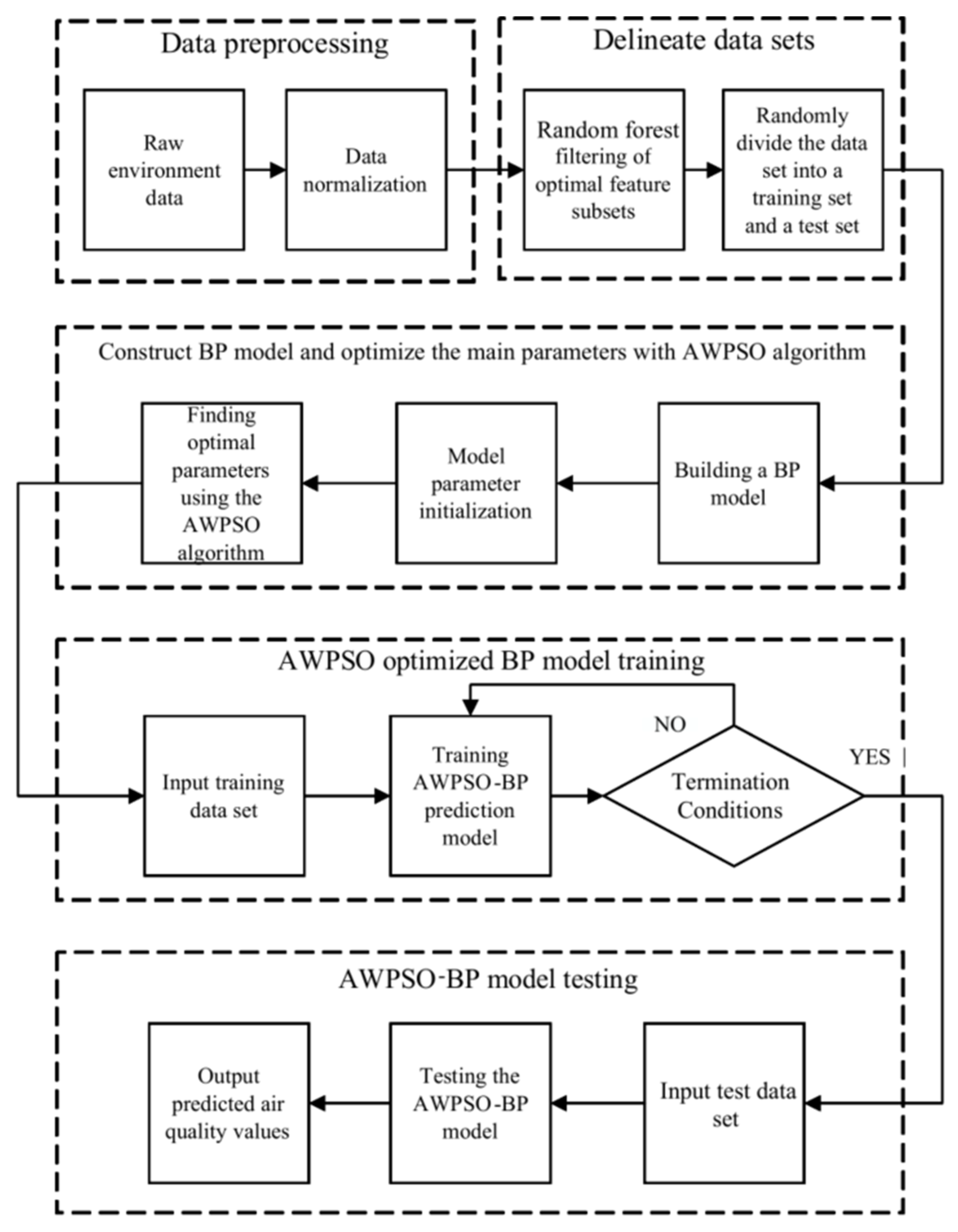
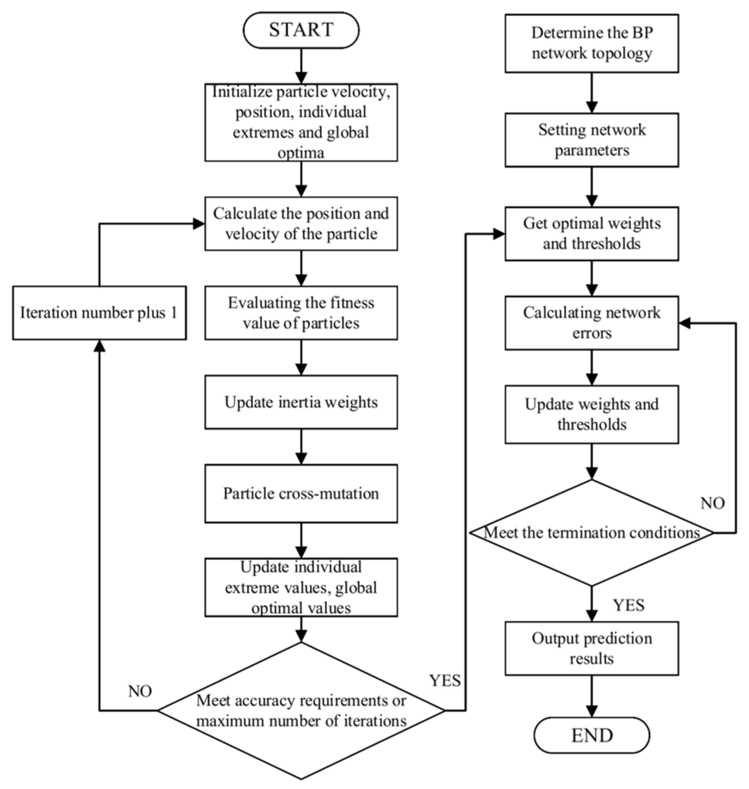
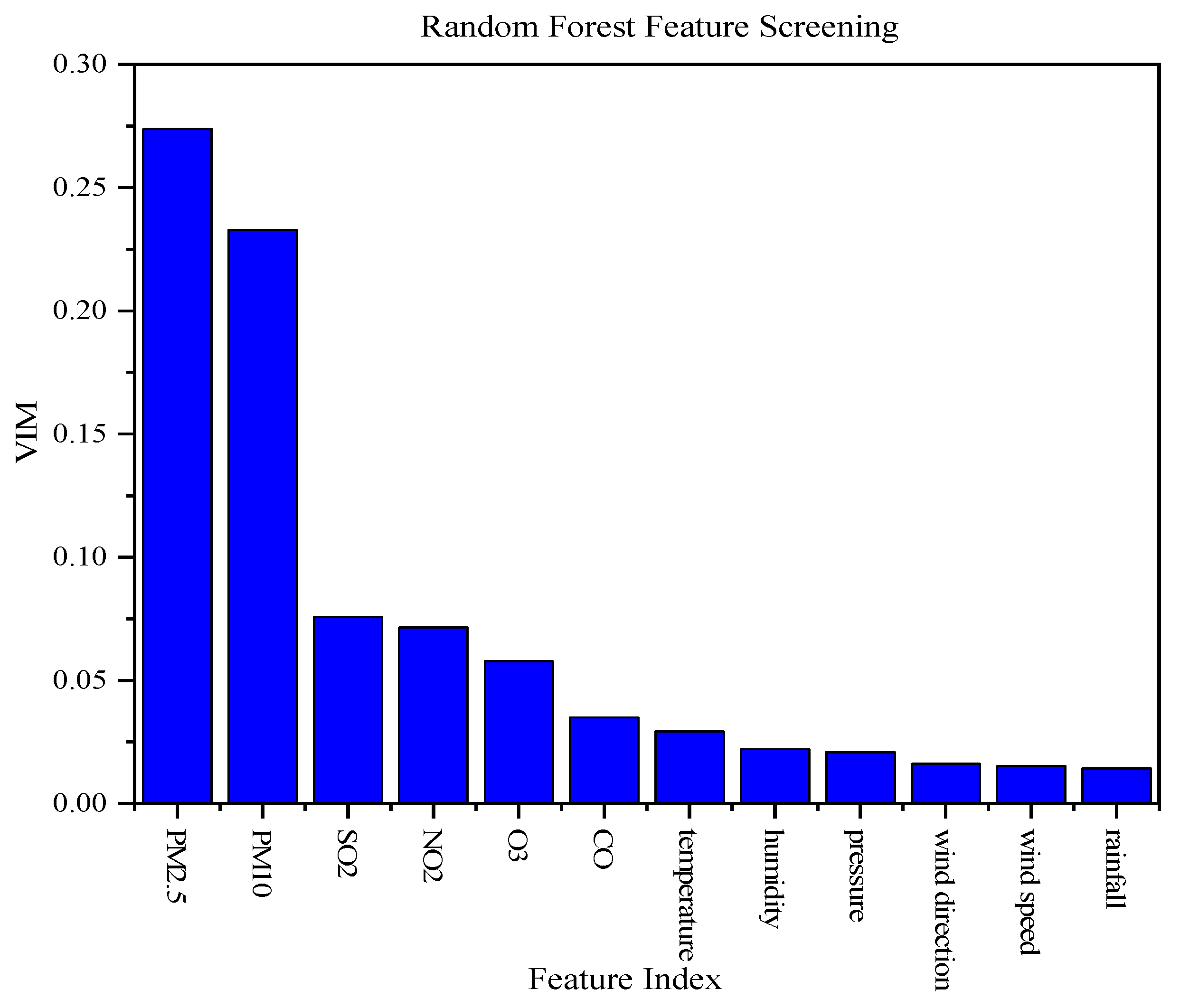
Despite extensive research efforts to enhance learning strategies, topological structures, and update mechanisms of PSO algorithms, conventional approaches continue to exhibit significant limitations, including slow convergence rates, susceptibility to local optima entrapment, and premature convergence phenomena. To address these computational challenges and enhance air quality prediction accuracy, this study proposes a comprehensive three-stage hybrid optimization framework. The methodology initially employs Random Forest (RF) algorithm to identify the optimal feature subset, effectively reducing dimensionality and eliminating redundant variables that may compromise prediction performance. Subsequently, the traditional PSO algorithm is enhanced through dynamically adaptive inertia weights and learning factors, while incorporating an adaptive mutation mechanism during particle search processes, thereby significantly improving global search capability and convergence efficiency while mitigating premature convergence risks. Finally, this enhanced PSO algorithm is utilized to simultaneously optimize both connection weights and threshold parameters of the BPNN, establishing a synergistic hybrid model that combines superior global optimization capabilities with robust nonlinear mapping strengths. Experimental validation conducted using air quality data from China, demonstrates that the proposed framework achieves faster convergence while effectively circumventing local optima limitations. The resulting model exhibits stable, rapid, efficient, and accurate air quality prediction capabilities, thereby overcoming the inherent deficiencies of traditional temporal prediction models and conventional hybrid approaches.

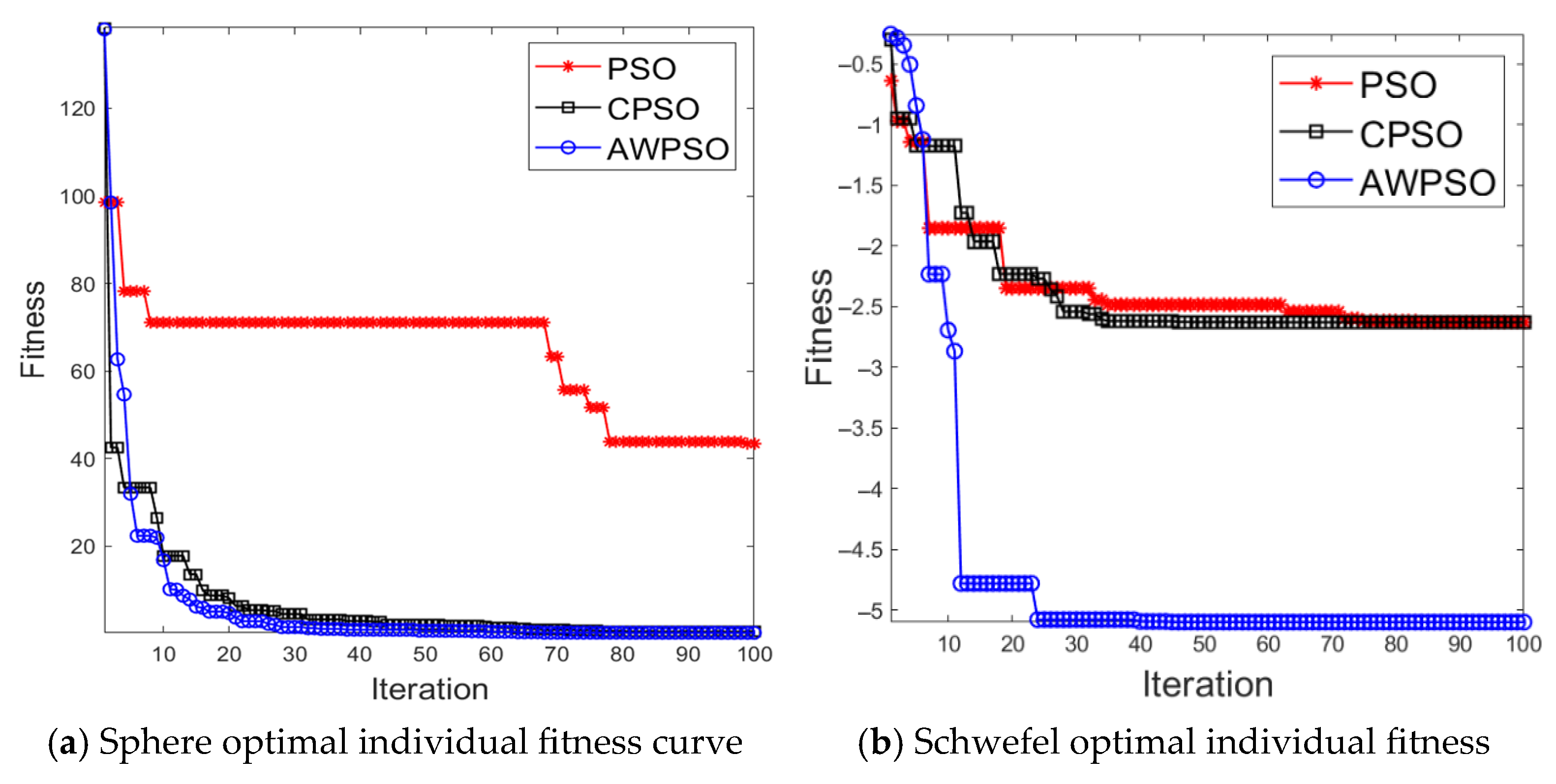
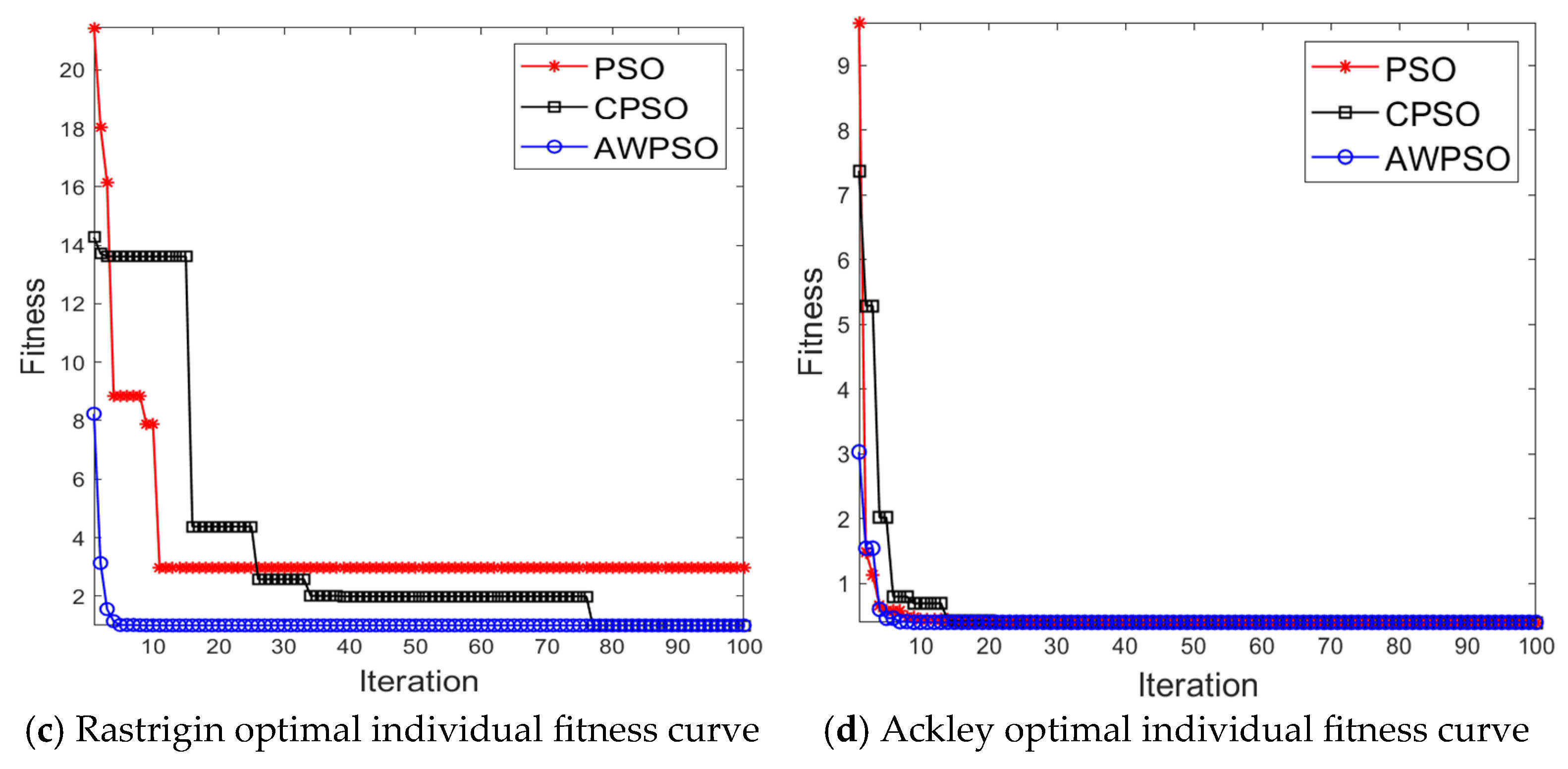
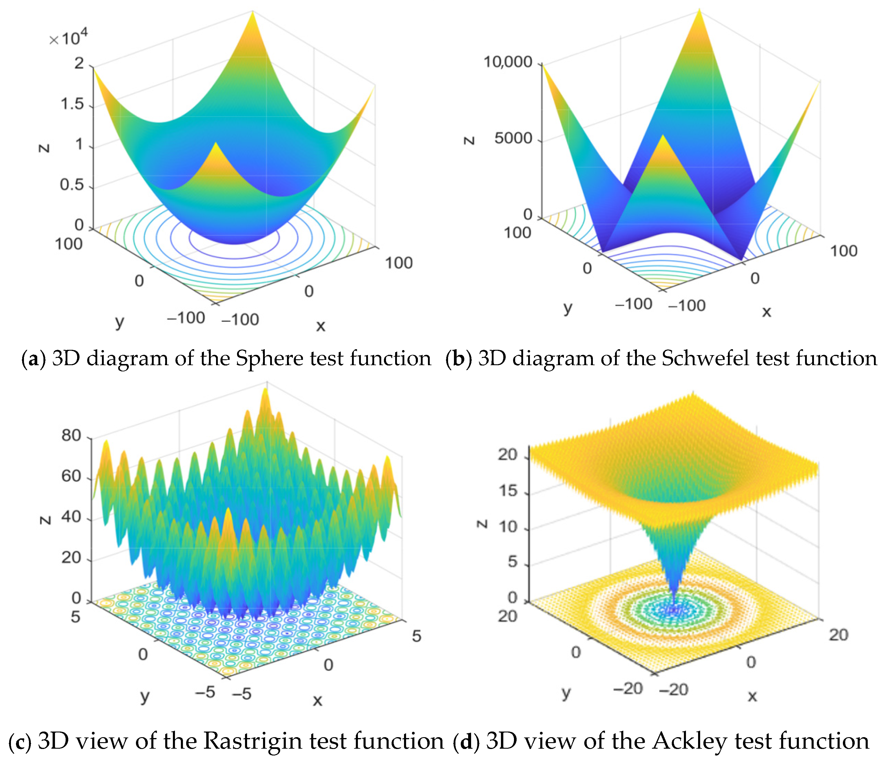
The rest of the paper is organized into five sections: Section 2 discusses the basic theory and methods of this work, including RFs, deep learning models, and improvements to the standard PSO algorithm. Section 3 describes building the prediction model and data preprocessing, followed by the results of filtering the input variables. Section 4 presents simulation results and analysis, including the validation of the adaptive-weight particle swarm algorithm (AWPSO) using four benchmark functions, and the simulation experimental results and discussion using air quality data from Shijiazhuang City. Section 5 presents the conclusions of the paper.

2. Theory

2.1. Random Forest

RF is characterized by fast computation, effective application to a wide range of nonlinear problems (involving complex higher-order interaction effects), and reliable identification of relevant predictive values from a large number of candidate variables. Therefore, this paper selects RF for feature screening of AQI impact factors. RF has been widely used in bioinformatics [40] and environmental science [41] for prediction and variable selection. As a machine learning integrated supervised learning method based on a bagging algorithm, RF uses a CART decision tree as the basis of forest construction, and adopts the Gini index to realize the node division of the CART decision tree, where the smaller the Gini index of nodes, the more ideal the effect of feature division [42]. Due to the characteristics of the decision tree, RF can be used not only for classification regression but also feature selection. Its basic principle is that there are put-back adoptions from the original dataset to obtain several subsets, training various base classifiers combining each subset, followed by obtaining the final classification results through voting of classifiers.

The calculation of the Gini index is shown in Equation (1):

$$Gin{i}^{\prime }(D)=1-{\displaystyle \sum _{i=1}^T{P}_{mi}^2}$$

(1)

where D denotes the air quality sample, $i$ represents the air quality class number, $T$ stands for the total number of air quality sample characteristics, and $p_{mi}$ denotes the subset of samples of the first class as a proportion of the whole sample.

After the decision tree is branched, it is assumed that the samples are divided into subsamples. The Gini index of the divided nodes is calculated by Equation (2):

$$Gin{i}^{\prime }(D)=P_{m1}Gini(D_1)+P_{m2}Gini(D_2)+\cdots +P_{mj}Gini(D_j)$$

(2)

The importance of a feature is expressed by calculating the difference in the Gini index before and after the node division, where the higher the difference, the higher the importance of the feature. The importance assessment value of the feature is usually expressed in terms of variable importance (VIM), which can be calculated by Equation (3):

$$VIM=\left|Gin{i}^{\prime }(D)-Gini(D)\right|$$

(3)

The computed results of each tree are weighted and averaged to evaluate the obtained features and rank their importance.

2.2. Back Propagation Neural Network Model

BPNN serves as a multi-layer feed-forward neural network that is trained based on the error BP algorithm, which is a kind of commonly applied neural network [43]. BPNN calculates output values considering the input layer data, initial weights, and thresholds, compares the current output value with the actual value, and then reverses the connection weights and thresholds. The structure of a three-layer BPNN (input layer, implicit layer, and output layer) is sufficient to fit most nonlinear systems, and the three-layer network structure has good parallelism and simple computation [43]. Therefore, a three-layer BPNN is used here for air quality prediction. Figure 1 gives the topology of the three-layer BPNN model.

The objective function of the BPNN is shown in Equation (4):

$$E={\displaystyle \frac{1}{2\times L}}{\displaystyle \sum _{i=1}^n{\displaystyle \sum _{j=1}^i{(y_{i,j}-{\widehat{y}}_{i,j})}^2}}$$

(4)

where $L$ is the size of the training sample, $i$ is the dimension of the output quantity $y$, and $y_{i,j}$ and ${\widehat{y}}_{i,j}$ are the actual and predicted values of AQI, respectively:

$$y_s=f(w_{1k}\times o_1+\cdots +w_{jk}\times o_j+\cdots +w_{nk}\times o_n+b_k)$$

(5)

where f denotes the activation function, $o_j$ is the output value of the hidden layer neurons, $w_{jk}$ is the weight, and $b_k$ is the bias.

To make the output value of AQI results close to the actual value, the weights and deviations of the network structure must be updated according to the training error. The update equations for hidden layer weights and biases are shown in Equations (6) and (7):

$$w_{jk}^{\prime }=w_{jk}-{\displaystyle \frac{\alpha }{s}}{\displaystyle \sum _{k-1}^s\Delta k\cdot o_j}$$

(6)

$$b_j^{\prime }=b_j-{\displaystyle \frac{1}{s}}{\displaystyle \sum _{k-1}^s\Delta k}$$

(7)

where represents the neuron number in the output layer, $w_{jk}^{\prime }$ is the neuron number associated with the first hidden layer neuron, is the update weight of the connection with the first hidden layer neuron and the first output layer neuron, $b_j^{\prime }$ is the update bias of the first number of output-layer neurons, $\Delta k$ is the training error, and $\Delta k=y_k-\stackrel{\wedge }{y_k}$.

In the parameter setting of the BP model, the number of BPNN layers is set to 3, in which the input layer has 6 input nodes, corresponding to 6 parameter variables of air quality. Considering the general empirical formula, we are allowed to initially set the implied layer number, and more reasonable results can be obtained after several simulation experiments [44]. The common empirical formula is shown in Equation (8):

$$q=\sqrt{M+L}+a$$

(8)

where $q$ represents the neuron number in the hidden layer, $M$ is the neuron number in the input layer, and $L$ is the neuron number in the output layer. $a$ is a fixed constant, which is set to 3.

2.3. Standard Particle Swarm Optimization Algorithm

The PSO algorithm is a new evolutionary computational method that simulates the foraging behavior of birds. The basic idea of the PSO algorithm is to find the optimal solution through collaboration and information-sharing among individuals in the population [33]. PSO is a global dynamic optimization-seeking computational method based on particle iterations that achieves the optimal spatial solution by seeking the global optimum and individual extrema during each iteration $p_g$ and individual extrema $p_i$ to continuously adjust its position and speed. Let the first particle i whose position in dimensional space is $X_i=(X_{i1,}{X}_{i2,}\dots X_{id,})$ and whose velocity is $V_i=(V_{i1,}{V}_{i2,}\dots V_{id,})$; the individual extremum is $P_i=(P_{i1,}{P}_{i2,}\dots P_{id,})$, and the global extremum of the population is $P_g=(P_{g1},P_{g2}\dots P_{gd})$. Figure 2 shows a particle in the population at the first k position updated in the second iteration, where $X_{id}^k$ is the current position of the particle, $X_{id}^{k+1}$ is the updated position, $V_{id}^k$ is the current velocity, $V_{id}^{k+1}$ is the current velocity, $V_g$ is the global extremum pointing to the $P_g$ is the velocity of $V_p$ is the velocity pointing to the individual extreme value of $P_i$ is the velocity of the $V_i$.

The velocity and position of the particle are updated based on Equations (9) and (10), whose iterative formulas are as follows:

$$V_{id}^{k+1}=w{V}_{id}^k+c_1{r}_1\left(P_{id}^k-X_{id}^k\right)+c_2{r}_2\left(P_{gd}^k-X_{id}^k\right)$$

(9)

$$X_{id}^{k+1}=X_{id}^k+V_{\mathrm{id}}^{k+1}$$

(10)

where Equation (9) is the velocity update equation, Equation (10) is the position update equation, $k$ is the number of current iterations, $w$ is the inertia weight factor, $c_1$ and $c_2$ called acceleration constants, $c_{1,}{c}_2\in [0,4]$, and $r_2$ are the random values of $r_{1,}{r}_2\in \left(0,1\right)$.

The particles keep tracking the individual extrema and global extrema in the solution space to search until a specified number of iterations is reached or a given error criterion is satisfied. To prevent the particle from searching blindly, the velocity of the particle is $\left[-V_{\max },V_{\max ,}\right]$, and its position is $\left[-X_{\max },V_{\max ,}\right]$.

2.4. Adaptive-Weight Particle Swarm Optimization Algorithm

Many scholars have proposed improvements to address the problems of PSO algorithms [38]. There are three main approaches to overcome the low convergence speed, the local optimization, and the maturation of PSO algorithms: (1) Adjusting the parameters of the PSO to balance the global detection and local exploitation capabilities; (2) Designing different types of topologies and changing particle learning patterns, thus increasing the diversity of populations; and (3) Combining PSO with other optimization algorithms to form a hybrid PSO algorithm. In this paper, the inertia weights and learning factors of PSO are improved, and the crossover and mutation operations of GA are introduced to improve the particle convergence speed and enhance the particle search ability. Thus, an air quality prediction model combining AWPSO and BPNN is developed.

The improvement of inertia weights can enhance the overall and local search ability exhibited by the algorithm. Specific to the standard PSO algorithm, the inertia weight presents a straight downtrend; thus, it exhibits a stronger global search ability in the initial iteration stage and a stronger local search ability in the later iteration stage. However, the method of decreasing the inertia weight coefficient is adopted too early, which leads to its poor global search ability in the later stage and local search ability in the earlier stage. In the initial search phase, the inertia weight coefficients are reduced nonlinearly, allowing the algorithm to possess a stronger global search capability in this phase and enter into local search rapidly. When iteration is stopped, the inertial weight coefficients start to decrease linearly, and the algorithm is capable of obtaining the optimal solution stably. Adjustment of the algorithm is achieved following Equation (11):

$$w=\left\{\begin{array}{c}{w}_{min}+\left(w_{max}-w_{min}\right)\times l_1\left(t\right),t<k\\ 2w_{min}+2\left(w_d-w_{min}\right)\times l_2\left(t\right),t\ge k\end{array}\right.$$

(11)

where $t$ is the number of iterations; $w_{\max }$ and $w_{min}$ are the largest and smallest values of the inertia weight coefficients, respectively; $l_1(t)$ represents a nonlinear function; $l_2(t)$ stands for a linear function; and $w_d$ is the initial inertia weight following the initial search.

The equations for $l_1(t)$ and $l_2(t)$ are shown in Equations (12) and (13):

$$l_1\left(t\right)=e^{-30\times {\left({\displaystyle \frac{t}{t_{max}}}\right)}^{10}}$$

(12)

$$l_2\left(t\right)=-{\displaystyle \frac{t}{t_{max}}}$$

(13)

where $t_{\max }$ is the maximum number of iterations.

To ensure particle diversity in early search phases, dynamic parameter adjustment is required. The algorithm must then rapidly converge to global optima in later stages. This study employs a tangent function for parameter modulation. The tangent function dynamically adjusts algorithmic parameters throughout optimization. This approach effectively balances global exploration and local exploitation. The tangent functions are as shown in Equations (14) and (15):

$$c_1=\left(c_{1\_start}-c_{1\_end}\right)\times tan\left\{0.875\times \left[1-{\left({\displaystyle \frac{t}{N}}\right)}^{0.5}\right]\right\}+c_{1\_end}$$

(14)

$$c_2=\left(c_{2\_start}-c_{2\_end}\right)\times arctan\left\{2.755\times \left[1-{\left({\displaystyle \frac{t}{N}}\right)}^{0.6}\right]\right\}+c_{2\_end}$$

(15)

PSO algorithms typically exhibit rapid early convergence rates. All particles quickly cluster near optimal positions. This clustering leads to significantly slower convergence in later stages. To address this limitation, genetic algorithm crossover and mutation operations are introduced. The mutation operation modifies single particle dimensions with specified probability. This mechanism enables particles to explore alternative search regions. The approach integrates GA’s global optimization capabilities with PSO’s local search efficiency. Local region convergence speed is substantially improved. Enhanced particle search ability results from this algorithmic synergy. The two algorithms achieve complementary performance benefits. Crossover operations are initially applied to particles with predetermined probability. For paired particles, the crossover process regarding position and velocity is shown in Equations (16) and (17):

$$\left\{\begin{array}{c}{X}_i^{k+1}={\beta }_1{X}_i^k+\left(1-{\beta }_1\right)X_j^k\\ X_j^{k+1}=\left(1-{\beta }_1\right)X_i^k+{\alpha }_1{X}_j^k\end{array}\right.$$

(16)

$$\left\{\begin{array}{c}{V}_i^{k+1}={\beta }_2{V}_i^k+\left(1-{\beta }_2\right)X_j^k\\ V_j^{k+1}=\left(1-{\beta }_2\right)V_i^k+{\alpha }_2{X}_j^k\end{array}\right.$$

(17)

The particles mutate with a certain probability to obtain new individuals by means of position and velocity crossover operations. This process is shown in Equations (18) and (19).

$$X_{ij}=\left\{\begin{array}{c}{X}_{ij}+\left(X_{ij}-X_{max}\right)Y\left(g\right),r_1\le 0.5\\ X_{ij}+\left(X_{min}-X_{ij}\right)Y\left(g\right),r_1>0.5\end{array}\right.$$

(18)

$$Y\left(g\right)=r_2\left(1-{\displaystyle \frac{k}{G_{max}}}\right)$$

(19)

where $X_{\max }$ and $X_{\min }$ denote the upper and lower bounds of particle $X_{ij}$, and $G_{\max }$ denotes the maximum number of evolutionary generations.

2.5. Proposed Model

2.5.1. Model Framework

In this paper, the collected air quality data are normalized. Then, the data are screened for optimal feature subsets using RF and are randomly sorted into the training set and the test set. Next, the constructed BP model is optimized using the AWPSO algorithm to find the optimal parameters. Finally, the optimized prediction model is the final air quality prediction model. Figure 3 shows the overall framework of the AWPSO optimized BPNN model.

2.5.2. Model Details

The specific training method for BPNN optimization based on the AWPSO algorithm is based on the principle that during each iteration, all particles update their positions according to the new rate calculated to move in a new direction, and the new positions are the new weights. Based on the weights of the network error set, a new network error set is obtained. To minimize the error in the network output layer, the particles are continuously moved within the range of weights (i.e., the network weights are continuously updated by moving search).

The connection weights and the thresholds are represented by the position vectors of the particles, where the size of the particles correspond to the number of ownership values and thresholds. The weight vectors and thresholds of the optimal particles are derived for each iteration, and the actual output values of the BPNN in this set of weight vectors and thresholds. The fitness function selects the Mean-Square Error (MSE) metric.

The steps of using AWPSO to optimize the BPNN algorithm are as follows:

Step 1: Given the input and output training sets of the network, perform normalization to determine the BPNN topology.

Step 2: Initialize the particle velocity, position, individual poles, and global poles, and set the particle position, velocity range, maximum number of iterations, and error accuracy.

Step 3: Determine the particle number in the population according to the structure and parameters regarding the neural network $n$ and inertia weights $w$, their maximum values $w_{\max }$ and minimum values $w_{\min }$, acceleration $c_1$ and $c_2$. Initialize the initial position of the particle by the uniform distribution function $x_{id}$, as well as $p_{id}$ and $p_{gd}$, and set the initial velocity of the particle to zero.

Step 4: Update the inertia weights, particle velocity, and position.

Step 5: Select a suitable fitness function to evaluate the adaptive value of each particle.

Step 6: Calculate the fitness function value for each particle. When the value is superior to the single optimal solution, the current value $p_{id}$ is used to update the single extreme value. When the individual is superior to the global optimum, the same method will replace the global extreme value $p_{gd}$.

Step 7: Calculate the particle velocity and position following Equations (9)–(11), (14) and (15), and perform the crossover and mutation operations of the particle according to Equations (16)–(19).

Step 8: If the largest iteration number or the smallest error accuracy is satisfied, stop the iteration, outputting the final weights and thresholds regarding the neural network; otherwise, go back to Step 4.

Step 9: Use the optimal values after AWPSO as the initial weights and thresholds of the BPNN. The BPNN is trained, together with the completion of related modeling.

Figure 4 gives a flow chart of the AWPSO-optimized BPNN.

3. Experiment

3.1. Data Sources and Pre-Processing

Air quality data were obtained from China Environmental Monitoring Station (www.cnemc.cn), including average daily PM_2.5, PM₁₀, O₃, CO, and SO₂ levels, as well as Nanjing AQI for the whole year of 2020–2021. These raw data suffer from many problems, such as incomplete and duplicate data. Some environmental sample data are shown in

Table 2. Selected environmental sample data.

Statistics	PM2.5 (μg/m3)	PM10 (μg/m3)	SO2 (μg/m3)	CO (mg/m3)	NO2 (μg/m3)	O3 (μg/m3)	AQI
Average	89.26	114.25	38.56	1.03	50.85	45.98	91.07
Median	69.23	56.06	32.64	0.96	46.23	31.13	108.23
Crowd	45.82	31.59	11.36	1.01	43.07	34.98	89.64
Standard	76.38	105.96	35.38	0.87	25.36	35.08	87.63
Maximum	172.36	218.27	40.23	1.51	77.07	77.42	230.56
Minimum	9.75	11.66	4.47	0.21	19.86	9.69	17.51

.

The data in the experiments were processed as follows:

1. Remove duplicate data. In the experiment, the data that are duplicates of the original data are deleted, and the duplicate-free data are kept.

2. Data filling. When detecting the air quality, data are missing due to the sensor itself as well as environmental effects. Given the smooth change in air ambient data over time, which usually do not change suddenly, the average ambient data for the previous and the subsequent hours are used to fill in missing portions of data. This is shown in Equation (20).

$$V_t={\displaystyle \frac{V_{t-1}+V_{t+1}}{2}}$$

(20)

where $V_{t-1}$ is the data at time $t$ of the previous hour, $V_t$ is the time $t$ for the missing value, and $V_{t+1}$ is the data at time $t$ data for the subsequent after.

After removing duplicates and filling in missing data, a total of 5628 data examples were collected. 4502 data from January 2020 to October 2021 were used as the training sample, and 1126 data from November and December 2021 were used as the test sample.

Due to the differences in environmental data, once unprocessed data are input into the prediction model, it will lead to slower training and poor prediction accuracy. Hence, for fastening the prediction model operation speed and enhancing the prediction accuracy, the input quantity must be normalized as shown in Equation (21):

$$Y\left(x\right)={\displaystyle \frac{x-min\left(x\right)}{max\left(x\right)-min\left(x\right)}}$$

(21)

where max(x) stands for the largest value in the data sample, min(x) represents the smallest value in the data sample, and $x$ is an arbitrary value in the data sample.

3.2. Experimental Design

The entire project was based on Python3. We used the PyTorch v1 library to develop and train our models. The experiments were conducted on a device equipped with an Intel Core i7 CPU and an NVIDIA GeForce RTX 3090 GPU (NVIDIA, Santa Clara, CA, USA).

This research uses the mean square error (RMSE), mean absolute error (MAE), and goodness-of-fit (R²) to assess the RF-AWPSO-BP model. The calculation method is as shown in Equations (22)–(24):

$$\mathrm{RMSE}=\sqrt{{\displaystyle \frac{{{\displaystyle \sum }}_{i=1}^n{\left(y_i-\widehat{y_i}\right)}^2}{n}}}$$

(22)

$$MAE={\displaystyle \frac{{{\displaystyle \sum }}_{i=1}^n\left|y_i-\widehat{y_i}\right|}{n}}$$

(23)

$$R^2=1-{\displaystyle \frac{{{\displaystyle \sum }}_{i=1}^n{\left(y_i-\widehat{y_i}\right)}^2}{{{\displaystyle \sum }}_{i=1}^n{\left(y_i-\overline{y_i}\right)}^2}}$$

(24)

where $y_i$ and ${\stackrel{\wedge }{y}}_i$ denote the actual value of the $i$ actual value and algorithm model output value of the second test, respectively, $n$ denotes the total test number, and ${\overline{y}}_i$ denotes the average value of the algorithm model output.

3.3. Predictor Screening

More dimensions of data will affect the prediction accuracy of ANN [45]. In this context, the RF algorithm evaluates the importance of each of the following environmental factors: PM_2.5, PM₁₀, SO₂, CO, NO₂, O₃, temperature, humidity, pressure, wind direction, wind speed, and rainfall. The optimal feature subset is filtered to enable the processing of moderate-dimensional data and enhance the prediction accuracy of the AWPSO-BP model. The RF code was run through python3 software to obtain the VIM of each indicator (

Table 3. The VIM of each indicator.

Indicator	VIM	Indicator	VIM
PM2.5	0.273776	Temperature	0.028245
PM10	0.232833	Humidity	0.022049
SO2	0.075757	Pressure	0.020996
NO2	0.07149	Wind direction	0.016189
O3	0.057766	Wind Speed	0.015286
CO	0.035083	Rainfall	0.014368

), as illustrated in Figure 5. Six indicators with VIM > 0.035 (PM_2.5, PM₁₀, SO₂, NO₂, CO, O₃) were screened, considering the RF results as the input samples for the model.

4. Results and Discussion

4.1. Algorithm Performance Analysis

The proposed AWPSO algorithm addresses the problems of the PSO algorithm, including its poor local search ability, tendency to fall into local extrema, and low search accuracy. Therefore, we select commonly used test functions to compare the AWPSO algorithm with the PSO and CPSO [46], as listed in

Table 4. Global optimization success rate of the three algorithms.

Global Optimization Success Rate	PSO (%)	CPSO (%)	AWPSO (%)
f1	67.6	98.6	100
f2	68.5	96.4	100
f3	76.3	98.8	99.8
f4	88.6	89.7	100

. We set the size of all three algorithms to 20, and $c_1=c_2=1.49455$. The largest iteration number is 100. Figure 6a–d represent the optimal individual fitness curves of the Sphere, Schwefel, Rastrigin, and Ackley test functions, and Figure 7a–d show the 3D plots of each test function, respectively.

The Sphere test function is a single-peaked function with a unique global minimum. The experimental results in Figure 6a show that the PSO algorithm frequently falls into local minima, whereas the CPSO algorithm and the AWPSO algorithm can find the global optimum very quickly. Although the AWPSO algorithm is only slightly inferior to the CPSO algorithm in the early stage, it has a faster search speed and higher accuracy in the middle and late stage, indicating an improved global search capability due to the other two algorithms.

Figure 7b shows that Schwefel is a continuous, smooth, multi-peaked function. From Figure 7b, it can be seen that the AWPSO algorithm converges slower in the early stage than the PSO and CPSO algorithms but has a faster convergence rate in the later stage, whereas both the PSO and CPSO algorithms fall into local minima during the optimization process.

Figure 7c, we can conclude that Rastrigin is also a multi-peaked function. As there are many local optima in the Rastrigin function, the algorithm can be easily caught in local optima in the process of finding the optimal value. However, as seen in Figure 6c, the PSO and CPSO algorithms fall into local extremes, whereas AWPSO quickly finds the global optimal solution. As seen in Figure 7d, the Ackley function has many local optima, and the independent variables are independent of each other. As seen in Figure (d), the AWPSO algorithm converges faster. The improved algorithm exhibits a strong global optimum–finding ability, has a reduced probability of falling into local optima, introduces the crossover and variation operation of the GM to improve the population diversity, and shows improved performance in the middle and late stages.

Therefore, as shown in Figure 6a–d, the PSO algorithm is usually caught in local extremes, whereas the other two algorithms are capable of finding the global optimal solution quickly. As the iteration number increases, the AWPSO algorithm obtains the optimal global solution with the least number of iterations among the four tested functions; the number of iterations basically does not exceed 20, showing a good optimization capability.

Table 4 shows the success rate (i.e., likelihood of obtaining the optimal test function value as a percentage) of the three algorithms. The calculation formulas for the indicators in Table 4 are shown in Equations (26)–(28). The PSO global optimization success rate is the lowest, whereas that of the AWPSO algorithm is the highest. The likelihood that the AWPSO algorithm falls into a local optimum is reduced by 32.4%, thus improving the accuracy of the algorithm model prediction. Therefore, it can be concluded from Figure 7 and Table 4 that the AWPSO algorithm solves the poor local search ability exhibited by the PSO algorithm and its likelihood of falling into local optima, improves its search accuracy, obtains a high iteration success rate, and has good stability.

$$f_1\left(x\right)={\displaystyle \sum }_{i=1}^D\left(x_i^2-10\cos \left(2\pi x_i\right)+10\right)$$

(25)

$$f_2\left(x\right)={\displaystyle \sum }_{i=1}^D{x}_i^2$$

(26)

$$f_3\left(x\right)=-aexp\left(-b\sqrt{{\displaystyle \frac{1}{d}}{\sum }_{i=1}^d{x}_i^2}\right)-exp({\displaystyle \frac{1}{d}}{\sum }_{i=1}^{d}cos\left(c{x}_i\right))$$

(27)

$$f_4\left(x\right)={\displaystyle \sum }_{i=1}^D\left|x_i\right|+{\displaystyle \prod }_{i=1}^D\left|x_i\right|$$

(28)

In summary, the proposed AWPSO algorithm has a certain improvement in both the search accuracy and convergence speed in dealing with high-latitude multi-peak issues. In solving the single-peak problem, the convergence speed is slower in the early stage, but there is an obvious improvement in search ability in the later stage, which proves the dependence of the solution performance exhibited by the improved algorithm on the other two algorithms, whether for single-peak or multi-peak functions.

4.2. Comparison of Convergence

This experiment uses the AWPSO algorithm to optimize the BPNN in terms of weights and thresholds. To compare the performance of different algorithms for parameter-optimization of the BPNN, the standard PSO algorithm and the AWPSO algorithm are chosen in this paper.

The PSO algorithm parameters are as follows: $c_1=c_2=2$ (i.e., the particle number is 20); the particle velocity range is $\left[-\mathrm{1,1}\right]$, the particle position range is $\left[-\mathrm{5,5}\right],$ and the BPNN is optimized via the PSO algorithm. The training of the AWPSO-BPNN was based on the following parameter settings: $c_{1\_start}=2.5$, $c_{1\_end}=0.5$, $c_{2\_start}=1$, $c_{2\_end}=3$, $w_{\min }=0.5$, $w_{\max }=1$, and the largest iteration number is 200.

Figure 8 displays the variation curves of the MSE with iteration number when the BPNN, PSO-BP, AWPSO-BP, and RF-AWPSO-BP models are trained. The BPNN model, after reaching a certain error, exhibits a slow convergence speed despite the MSE decreasing with the increase in generations, and the optimal solution can be hardly found. The AWPSO-BP algorithm model converges fast and with low error compared with the PSO-BP algorithm model, which can effectively perform the global optimization search. Although the AWPSO-BP and RF-AWPSO-BP models are very close to each other, the RF-AWPSO-BP model has a smaller error and is easier to perform global optimization. Accordingly, the RF-AWPSO-BP model outperforms the BP model, the standard PSO-BPNN model, and the AWPSO model.

4.3. Performance Comparison of Prediction Models at Different Time Intervals

To analyze and evaluate the prediction performance of the RF-AWPSO-BP prediction model for different time intervals, we divided the test samples into 1, 4, 12, and 24 h for predicting air quality (i.e., AQI). Generally speaking, the air quality of a day varies with time, so if the model can accurately predict it over time, it has an outstanding prediction performance. We compare the output values of the AWPSO-BP model and the RF-AWPSO-BP model with the true values, as shown in Figure 9.

From Figure 9, it can be seen that the error between the predicted and true values of the AWPSO-BP model increases with time, owing to the original dataset being directly imported into the AWPSO-BP model without feature selection of the original dataset, resulting in the prediction error of the prediction model gradually becoming larger with time. The RF-AWPSO-BP model, on the other hand, has a larger error between the predicted and true values as time increases, but the error changes are smaller because the optimal feature subset is obtained by using the RF algorithm for feature selection of the original dataset. Both prediction models have lower RMSEs and MAEs within 1 h, and higher R² values (

Table 5. Comparison results of different time intervals.

Time Interval (h)	RMSE (μg/m3)		MAE (μg/m3)		R2 (%)
	AWPSO-BP	RF-AWPSO-BP	AWPSO-BP	RF-AWPSO-BP	AWPSO-BP	RF-AWPSO-BP
1	2.67	0.99	2.52	0.98	95.6	97.2
4	5.10	1.94	4.92	1.76	91.5	96.7
12	7.27	2.46	7.18	2.34	89.6	95.4
24	9.62	2.58	9.08	2.42	84.2	94.8

). However, as time increases, the RMSE and MAE of the AWPSO-BP model become larger, and the fit (R²) becomes lower, whereas the RMSE, MAE and R² of the RF-AWPSOBP model change less, indicating the superiority of the RF-AWPSO-BP model in terms of prediction performance.

4.4. Comparison of Prediction Results of Different Models

To analyze the forecasting ability exhibited by the RF-AWPSO-BP-based hybrid model, we choose BPNN, PSO-BPNN, and AWPSO-BPNN to compare with 1 h time series. Although BPNN and PSO-BPNN have been widely used in the field of forecasting, they both have disadvantages, such as low generalization, poor stability, and overfitting, leading to low accuracy of their prediction models. The model proposed in this paper can relatively solve the above-mentioned problems and improve the prediction accuracy of air quality. The trained models are used to predict future air quality, and the predicted values are compared with the actual values. Figure 10 shows the comparison results between the predicted and actual values of the four algorithm models, and Figure 11 shows the error comparison of the four algorithm models. Figure 10 and Figure 11 show that the predicted and actual values of the RF-AWPSO-BP algorithm model fit better, and the fitted curves match better and have a smaller error compared with the BP algorithm model, PSO-BP algorithm model, and AWPSO-BPS algorithm model. The results show that compared with the BP, PSO-BP, and AWPSO-BP models, the RF-AWPSO-BP model proposed in this paper has stronger learning ability and good generalization ability and can predict air quality concentration more accurately.

To further compare the prediction performance of the different models in this work, three evaluation metrics are introduced in the paper: RMSE, MAE, and R².

Table 6. Comparison of metrics for the performance of the three algorithms for prediction models.

Algorithm Model	RMSE	MAE	R2 (%)
BP	10.22	10.02	82.7
PSO-BP	6.75	6.6	91.4
AWPSO-BP	3.71	3.58	95.2
RF-AWPSO-BP	1.05	0.9	97.5

compares these metrics to evaluate the performance of the different prediction algorithm models.

From Table 6, the RMSE and MAE of RF-AWPSO-BPNN are much lower than those of the other three algorithm models, by 9.17 μg/m³, 5.7 μg/m³, 2.66 μg/m³; and 9.12 μg/m³, 5.7 μg/m³, and 2.68 μg/m³, respectively, indicating that the predicted values are closest to the actual values, with the best prediction accuracy and the least prediction error. Meanwhile, the fit of the RF-AWPSO-BP algorithm model is 97.5%, which is 14.8%, 6.1%, and 2.3% higher than that of the BP, PSO-BP, and AWPSO-BP models, respectively, revealing the better prediction performance of the proposed model. Therefore, the RF-AWPSO-BPNN model exhibits excellent prediction performance and is capable of meeting air quality prediction.

4.5. Sensitivity Analysis

To test the applicability of the proposed RF-AWPSO-BP optimized model for different datasets, we next perform sensitivity analysis, which commonly serves to investigate and analyze how parameter variation affects prediction model performance. As the variation of PM_2.5 concentration has a significant impact on air quality prediction, we choose PM_2.5 as the input variable. The sensitivity of the variables to the tested parameters is calculated as shown in Equation (29):

$$\nu ={\displaystyle \frac{{{\displaystyle \sum }}_{t=1}^n\left|Y_t^{\prime }-Y_t\right|}{n}}$$

(29)

where $\nu$ denotes the rate of change; $Y_t$ and $Y_t^{\prime }$ denote the values of the output variables before and after the time change, respectively; and $n$ denotes the total number of experiments.

We vary the PM_2.5 inputs as −50%, −30%, −10%, 10%, 30%, and 50%, and keep the remaining five inputs constant; thus, we can derive the rate of change in the impact of PM_2.5 on AQI. The rates of change for each model with different PM_2.5 inputs are shown in Figure 12, which show that the change in air quality concentration predicted using the RF-AWPSO-BP model is relatively small, with the largest change rate being 0.182. In comparison, the largest change rate in air quality concentration predicted using the AWPSO-BP, PSO-BP, and BP models is 0.312, 0.661, and 0.934, respectively. Thus, the RF-AWPSO-BP model is the least sensitive to changes in the input values and has the least variability and stability. Therefore, the RF-AWPSO BP model is capable of effectively avoiding inaccurate concentration prediction values due to algorithm defects.

5. Conclusions

As the problem of air pollution has seriously affected people’s health and economic development, the prediction and control of air pollution have now become an urgent direction in research today. Although the traditional BP model is a widely used prediction method, it is prone to being caught in minimal value and slow convergence speed, adding difficulty in accurately predicting AQI. The combined prediction model based on RF-AWPSO-BPNN proposed in this paper is capable of improving the accuracy of air quality prediction. By analyzing and comparing AWPSO simulation tests and experimental data, the following conclusions are drawn.

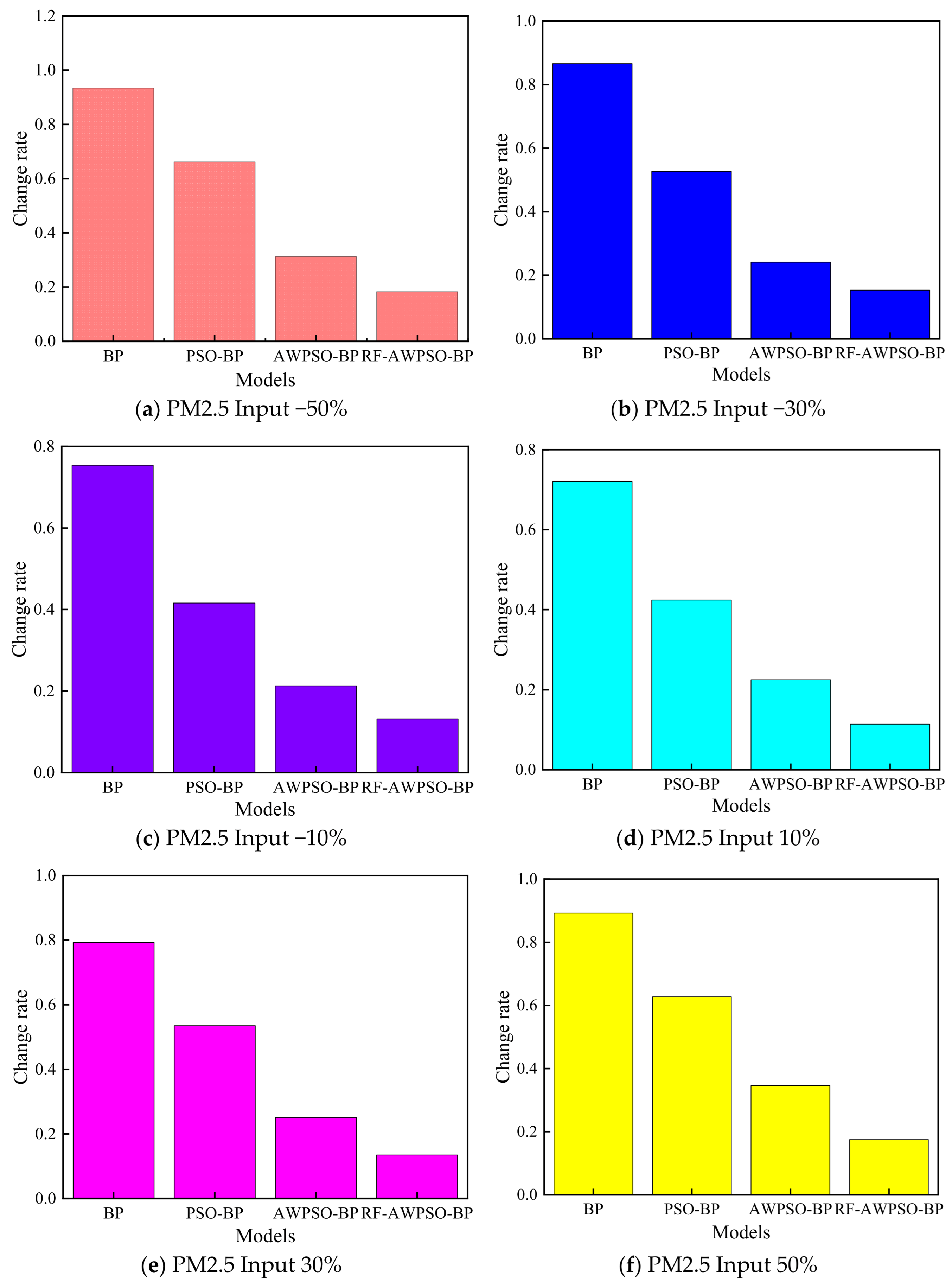
(1) The optimal feature subset is obtained by feature extraction of the original data through RF, which contributes to an effective improvement in AQI prediction accuracy.

(2) The PSO algorithm is chosen to optimize the BPNN for its defects and obtaining the best weights and thresholds.

(3) Due to the low convergence speed, local optimization, and premature maturation of the PSO algorithm, the study improves the inertia weights and learning factors and introduces the crossover and variation operations of GA in the particle search process to enhance the particle convergence speed and improve the particle search capability.

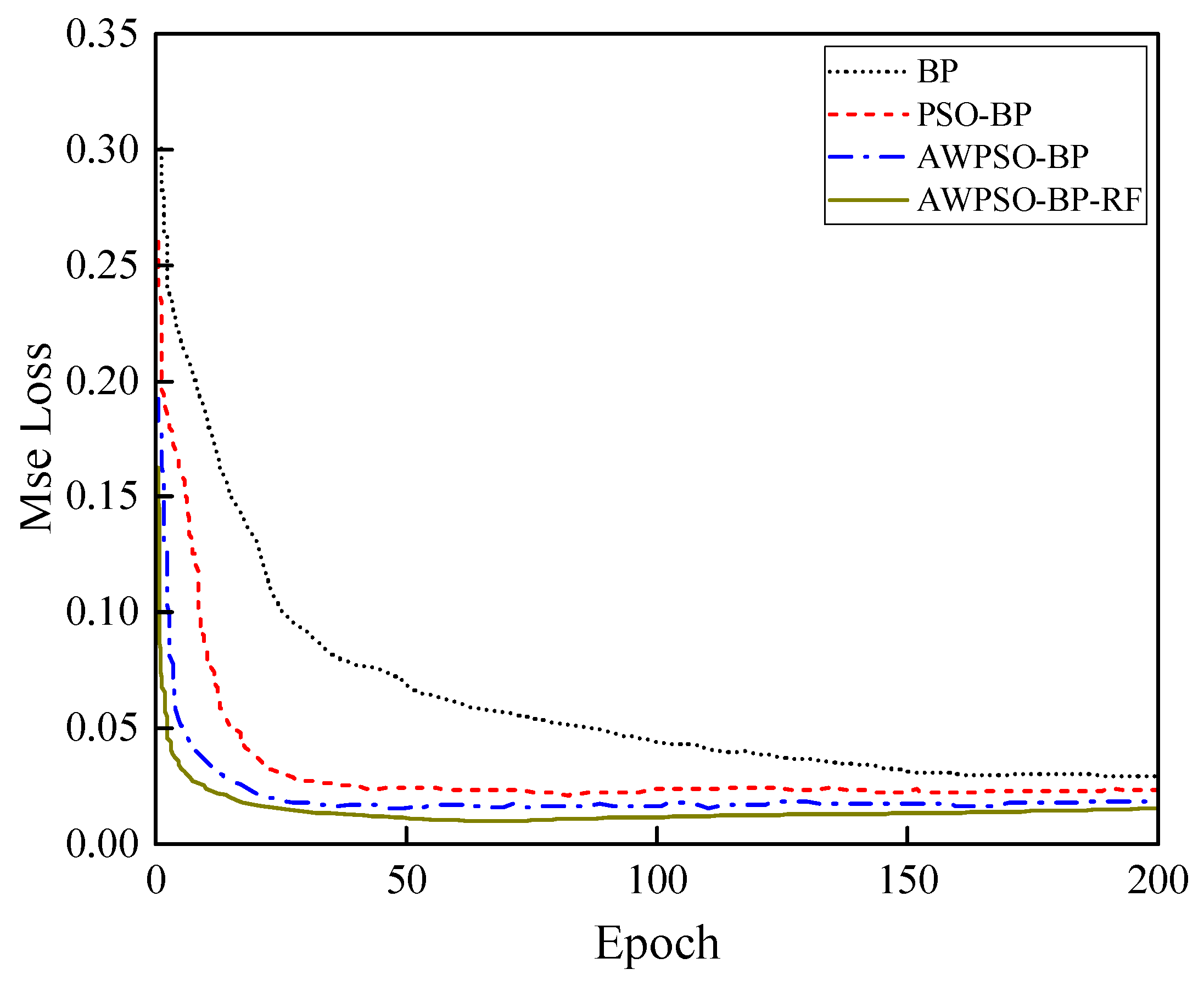
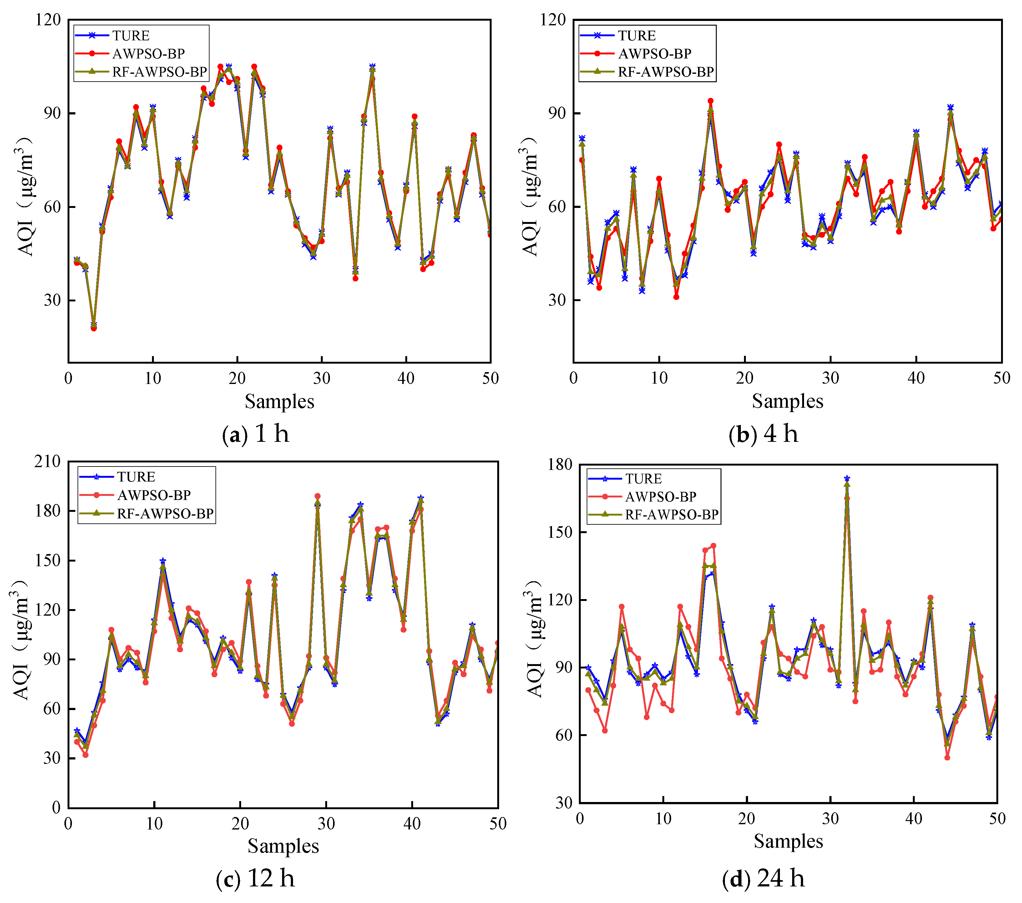
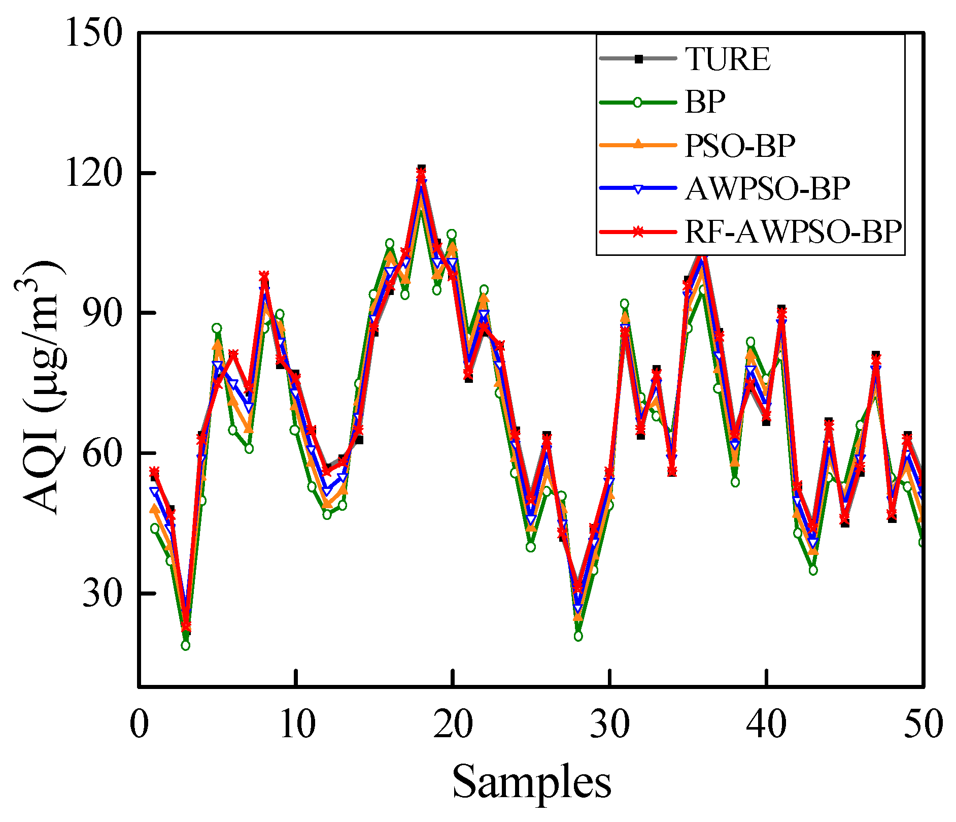
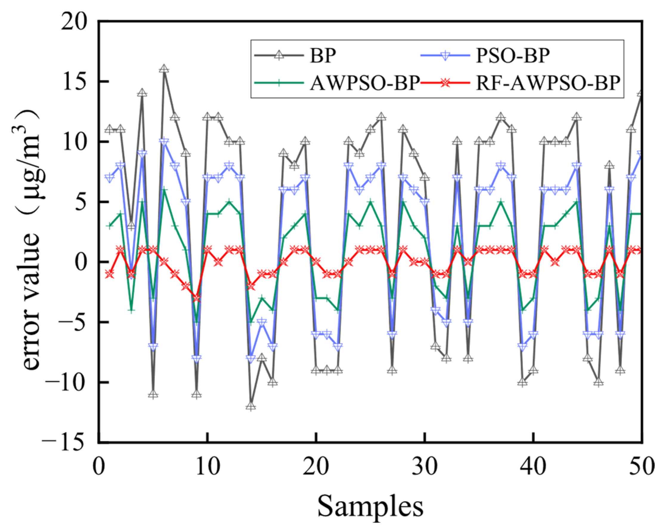
(4) Through comparison experiments, it is found that the proposed RF-AWPSO-BP hybrid model greatly improves the prediction performance, and the predicted and true values exhibit a strong fitting degree.

The above findings prove that the hybrid prediction model has high accuracy for AQI prediction, which is of practical application for the prediction and control of air pollution.

The proposed model offers significant practical value to multiple stakeholders in environmental management and public health sectors. Environmental protection agencies and regulatory bodies can leverage the improved AQI prediction accuracy to enhance their air quality monitoring capabilities and develop more effective pollution control policies. Public health officials can utilize the reliable forecasting results to establish better early warning systems and health advisories. Additionally, weather and environmental forecasting services can incorporate our model to provide more accurate air quality forecasts to the general public, enabling citizens to make informed decisions about outdoor activities and health protection measures. The research also contributes to the broader scientific community by advancing methodological approaches in environmental prediction modeling, while offering practical solutions for smart city initiatives.

However, the air quality of a location is not only affected by its own historical data (temporal dimension), but also significantly affected by the transport of pollutants from surrounding areas (spatial dimension). This manuscript does not adequately consider the interactions in geospatial space. Future work will focus on improving long-term prediction capabilities. We plan to explore multi-scale modeling strategies to hierarchically process prediction tasks at different time scales. In addition, we will study how to effectively integrate multi-source external data such as weather forecasts to enhance the model’s ability to predict environmental changes. By combining ensemble learning methods with the long-term memory advantages of deep learning models, it is expected that a more robust long-term AQI prediction system will be built to provide decision support for environmental management and public health policy making.

References

1. Wang, J.Y.; Li, J.Z.; Wang, X.X.; Wang, J.; Huang, M. Air quality prediction using CT-LSTM. Neural Comput. Appl. 2021, 33, 4779–4792. [Google Scholar] [CrossRef]
2. Soh, P.W.; Chang, J.W.; Huang, J.W. Adaptive Deep Learning-Based Air Quality Prediction Model Using the Most Relevant Spatial-Temporal Relations. IEEE Access 2018, 6, 38186–38199. [Google Scholar] [CrossRef]
3. Yang, L.; Li, X.; Jareemit, D.; Liu, J. Vegetation Configuration Effects on Microclimate and PM2.5 Concentrations: A Case Study of High-Rise Residential Complexes in Northern China. Atmosphere 2025, 16, 672. [Google Scholar] [CrossRef]
4. Miguel, J.P.M.; de Blas, C.S.; Sipols, A.E.G. A forecast air pollution model applied to a hypothetical urban road pricing scheme: An empirical study in Madrid. Transp. Res. Part D Transp. Environ. 2017, 55, 21–38. [Google Scholar] [CrossRef]
5. Wang, W.W.; Cui, K.P.; Zhao, R.; Hsieh, L.T.; Lee, W.J. Characterization of the Air Quality Index for Wuhu and Bengbu Cities, China. Aerosol Air Qual. Res. 2018, 18, 1198–1220. [Google Scholar] [CrossRef]
6. Kumar, P.; Singh, A.B.; Arora, T.; Singh, S.; Singh, R. Critical review on emerging health effects associated with the indoor air quality and its sustainable management. Sci. Total Environ. 2023, 872, 162163. [Google Scholar] [CrossRef] [PubMed]
7. Abolhasani, R.; Araghi, F.; Tabary, M.; Aryannejad, A.; Mashinchi, B.; Robati, R.M. The impact of air pollution on skin and related disorders: A comprehensive review. Dermatol. Ther. 2021, 34, e14840. [Google Scholar] [CrossRef] [PubMed]
8. Xi, J.; Chen, Y.; Li, J. BP-SVM air quality combination prediction model based on binary linear regression. Int. J. Earth Sci. Eng. 2016, 9, 1194–1199. [Google Scholar]
9. Wu, Q.L.; Lin, H.X. A novel optimal-hybrid model for daily air quality index prediction considering air pollutant factors. Sci. Total Environ. 2019, 683, 808–821. [Google Scholar] [CrossRef] [PubMed]
10. Zhang, Z.; Zeng, Y.; Yan, K. A hybrid deep learning technology for PM2.5 air quality forecasting. Environ. Sci. Pollut. Res. 2021, 28, 39409–39422. [Google Scholar] [CrossRef] [PubMed]
11. He, H.D.; Lu, W.Z.; Xue, Y. Prediction of particulate matter at street level using artificial neural networks coupling with chaotic particle swarm optimization algorithm. Build. Environ. 2014, 78, 111–117. [Google Scholar] [CrossRef]
12. Bartzis, J.; Andronopoulos, S.; Sakellaris, I. Source Term Estimation for Puff Releases Using Machine Learning: A Case Study. Atmosphere 2025, 16, 697. [Google Scholar] [CrossRef]
13. Abhilash, M.S.K.; Thakur, A.; Gupta, D.; Sreevidya, B. Time Series Analysis of Air Pollution in Bengaluru Using ARIMA Model. In Proceedings of the Ambient Communications and Computer Systems, Singapore, 10–11 August 2018; pp. 413–426. [Google Scholar]
14. Liu, B.; Zhao, Q.B.; Jin, Y.Q.; Shen, J.Y.; Li, C.Y. Application of combined model of stepwise regression analysis and artificial neural network in data calibration of miniature air quality detector. Sci. Rep. 2021, 11, 3247. [Google Scholar] [CrossRef] [PubMed]
15. Liu, B.C.; Binaykia, A.; Chang, P.C.; Tiwari, M.K.; Tsao, C.C. Urban air quality forecasting based on multidimensional collaborative Support Vector Regression (SVR): A case study of BeijingTianjin-Shijiazhuang. PLoS ONE 2017, 12, e0179763. [Google Scholar] [CrossRef]
16. Hualong, L.; Miao, L.; Kai, Z.; Xianwang, L.; Xuanjiang, Y.; Zelin, H.; Panpan, G. Construction Method and Performance Test of Prediction Model for Laying Hen Breeding Environmental Quality Evaluation. Smart Agric. 2020, 2, 37–47. [Google Scholar]
17. Wan, R. Research on Air Quality Prediction Based on Neural Networks. Front. Comput. Intell. Syst. 2024, 8, 43–46. [Google Scholar] [CrossRef]
18. Cabaneros, S.M.; Calautit, J.K.; Hughes, B.R. A review of artificial neural network models for ambient air pollution prediction. Environ. Model. Softw. 2019, 119, 285–304. [Google Scholar] [CrossRef]
19. Ning, M.; Guan, J.H.; Liu, P.Z.; Zhang, Z.P.; O’Hare, G.M.P. GA-BP Air Quality Evaluation Method Based on Fuzzy Theory. Comput. Mater. Contin. 2019, 58, 215–227. [Google Scholar] [CrossRef]
20. Liu, H.; Li, Q.; Yu, D.; Gu, Y. Air Quality Index and Air Pollutant Concentration Prediction Based on Machine Learning Algorithms. Appl. Sci. 2019, 9, 4069. [Google Scholar] [CrossRef]
21. Gupta, N.S.; Mohta, Y.; Heda, K.; Armaan, R.; Valarmathi, B.; Arulkumaran, G. Prediction of Air Quality Index Using Machine Learning Techniques: A Comparative Analysis. J. Environ. Public Health 2023, 2023, 4916267. [Google Scholar] [CrossRef]
22. Du, S.; Li, T.; Yang, Y.; Horng, S.J. Deep Air Quality Forecasting Using Hybrid Deep Learning Framework. IEEE Trans. Knowl. Data Eng. 2021, 33, 2412–2424. [Google Scholar] [CrossRef]
23. Xu, J.; Li, X.; Lu, W.; Wei, X.; Chen, G.; Li, Y. A heterogeneous two-layer graph convolution model for turning traffic prediction with missing data. Transp. B Transp. Dyn. 2025, 13, 2497941. [Google Scholar] [CrossRef]
24. Xu, J.; Li, Y.; Lu, W.; Wu, S.; Li, Y. A heterogeneous traffic spatio-temporal graph convolution model for traffic prediction. Phys. A Stat. Mech. Its Appl. 2024, 641, 129746. [Google Scholar] [CrossRef]
25. Wang, X.; Wang, B. Research on prediction of environmental aerosol and PM2.5 based on artificial neural network. Neural Comput. Appl. 2019, 31, 8217–8227. [Google Scholar] [CrossRef]
26. Maleki, H.; Sorooshian, A.; Goudarzi, G.; Baboli, Z.; Tahmasebi Birgani, Y.; Rahmati, M. Air pollution prediction by using an artificial neural network model. Clean Technol. Environ. Policy 2019, 21, 1341–1352. [Google Scholar] [CrossRef] [PubMed]
27. Li, L.; Zhang, Y.M.; Fung, J.C.H.; Qu, H.M.; Lau, A.K.H. A coupled computational fluid dynamics and back-propagation neural network-based particle swarm optimizer algorithm for predicting and optimizing indoor air quality. Build. Environ. 2022, 207, 108533. [Google Scholar] [CrossRef]
28. Chen, P.S.; Zheng, Y.J.; Li, L.; Jing, T.; Du, X.X.; Tian, J.Z.; Zhang, J.X.; Dong, M.Y.; Fan, J.C.; Wang, C.; et al. Prediction of PM2.5 Mass Concentration Based on the Back Propagation (BP) Neural Network Optimized by t-Distribution Controlled Genetic Algorithm. J. Nanoelectron. Optoelectron. 2020, 15, 432–441. [Google Scholar] [CrossRef]
29. Yang, Y.; Wang, G.; Yang, Y. Parameters optimization of polygonal fuzzy neural networks based on GA-BP hybrid algorithm. Int. J. Mach. Learn. Cybern. 2014, 5, 815–822. [Google Scholar] [CrossRef]
30. Xu, X.M.; Peng, L.Y.; Ji, Z.S.; Zheng, S.P.; Tian, Z.X.; Geng, S.P. Research on Substation Project Cost Prediction Based on Sparrow Search Algorithm Optimized BP Neural Network. Sustainability 2021, 13, 13746. [Google Scholar] [CrossRef]
31. Bi, Y.; Wang, S.; Zhang, C.; Cong, H.; Qu, B.; Li, J.; Gao, W. Safety and reliability analysis of the solid propellant casting molding process based on FFTA and PSO-BPNN. Process Saf. Environ. Prot. 2022, 164, 528–538. [Google Scholar] [CrossRef]
32. Lu, J.; Huang, M.; Wu, W.; Wei, Y.; Liu, C. Application and Improvement of the Particle Swarm Optimization Algorithm in Source-Term Estimations for Hazardous Release. Atmosphere 2023, 14, 1168. [Google Scholar] [CrossRef]
33. Xiao, M.; Luo, R.; Chen, Y.; Ge, X. Prediction model of asphalt pavement functional and structural performance using PSO-BPNN algorithm. Constr. Build. Mater. 2023, 407, 133534. [Google Scholar] [CrossRef]
34. Yingying, G.; Hexiang, Q.; Suwen, L.; Fusheng, M. Application of BP neural network based on particle swarm optimization in atmospheric NO2 concentration prediction. J. Atmos. Environ. Opt. 2022, 17, 230–240. [Google Scholar]
35. Cai, Z.; Feng, G.; Wang, Q. Based on the Improved PSO-TPA-LSTM Model Chaotic Time Series Prediction. Atmosphere 2023, 14, 1696. [Google Scholar] [CrossRef]
36. Jiang, H.; Yan, Z.; Liu, X. Melt index prediction using optimized least squares support vector machines based on hybrid particle swarm optimization algorithm. Neurocomputing 2013, 119, 469–477. [Google Scholar] [CrossRef]
37. Sun, Y.; Gao, Y.; Shi, X. Chaotic Multi-Objective Particle Swarm Optimization Algorithm Incorporating Clone Immunity. Mathematics 2019, 7, 146. [Google Scholar] [CrossRef]
38. Sabat, S.L.; Ali, L.; Udgata, S.K. Integrated Learning Particle Swarm Optimizer for global optimization. Appl. Soft Comput. 2011, 11, 574–584. [Google Scholar] [CrossRef]
39. Li, M.; Zhang, H.; Liu, L.; Chen, B.; Guan, L.; Wu, Y. A Quantitative Structure-Property Relationship Model Based on Chaos-Enhanced Accelerated Particle Swarm Optimization Algorithm and Back Propagation Artificial Neural Network. Appl. Sci. 2018, 8, 1121. [Google Scholar] [CrossRef]
40. Li, J.J.; Xu, L.; Yang, C.H.; Jiang, Y. Transmembrane Protein Prediction Using N-Gram and Random Forests. J. Comput. Theor. Nanosci. 2014, 11, 2526–2534. [Google Scholar] [CrossRef]
41. Liu, Y.; Li, Y.P.; Yang, W.; Hu, J. Exploring nonlinear effects of built environment on jogging behavior using random forest. Appl. Geogr. 2023, 156, 102990. [Google Scholar] [CrossRef]
42. Qu, L.A.; Chen, Z.J.; Li, M.C. CART-RF Classification with Multifilter for Monitoring Land Use Changes Based on MODIS Time-Series Data: A Case Study from Jiangsu Province, China. Sustainability 2019, 11, 5657. [Google Scholar] [CrossRef]
43. Wang, Z.; Wu, J.; Wang, H.; Wang, H.; Hao, Y. Optimal Underwater Acoustic Warfare Strategy Based on a Three-Layer GA-BP Neural Network. Sensors 2022, 22, 9701. [Google Scholar] [CrossRef] [PubMed]
44. Sheela, K.G.; Deepa, S.N. Review on Methods to Fix Number of Hidden Neurons in Neural Networks. Math. Probl. Eng. 2013, 2013, 425740. [Google Scholar] [CrossRef]
45. Guha, S.; Jana, R.K.; Sanyal, M.K. Artificial neural network approaches for disaster management: A literature review. Int. J. Disaster Risk Reduct. 2022, 81, 103276. [Google Scholar] [CrossRef]
46. Alayi, R.; Mohkam, M.; Seyednouri, S.R.; Ahmadi, M.H.; Sharifpur, M. Energy/Economic Analysis and Optimization of On-Grid Photovoltaic System Using CPSO Algorithm. Sustainability 2021, 13, 12420. [Google Scholar] [CrossRef]
Figure 1. BPNN model.
Atmosphere 16 00870 g001
Figure 2. Schematic diagram of the position update of particles in a particle swarm.
Atmosphere 16 00870 g002
Figure 3. Framework of AWPSO-optimized BPNN prediction model.
Atmosphere 16 00870 g003
Figure 4. Flow chart of AWPSO-optimized BPNN.
Atmosphere 16 00870 g004
Figure 5. Importance of environmental sample characteristic variables (VIM ranking).
Atmosphere 16 00870 g005
Figure 6. Optimal individual fitness plots of each test function.
Atmosphere 16 00870 g006aAtmosphere 16 00870 g006b
Figure 7. Three-dimensional diagrams of each test function.
Atmosphere 16 00870 g007
Figure 8. MSE curves of different training models.
Atmosphere 16 00870 g008
Figure 9. Air quality prediction results for different time intervals.
Atmosphere 16 00870 g009
Figure 10. Comparison of four models in terms of the predicted and actual values.
Atmosphere 16 00870 g010
Figure 11. Comparison of the four algorithm models in terms of error values.
Atmosphere 16 00870 g011
Figure 12. Rate of change in each model with different inputs.
Atmosphere 16 00870 g012