
Air Temperature Extremes in the Mediterranean Region (1940–2024): Synoptic Patterns and Trends


Abstract
1. Introduction
2. Materials and Methods
2.1. Data
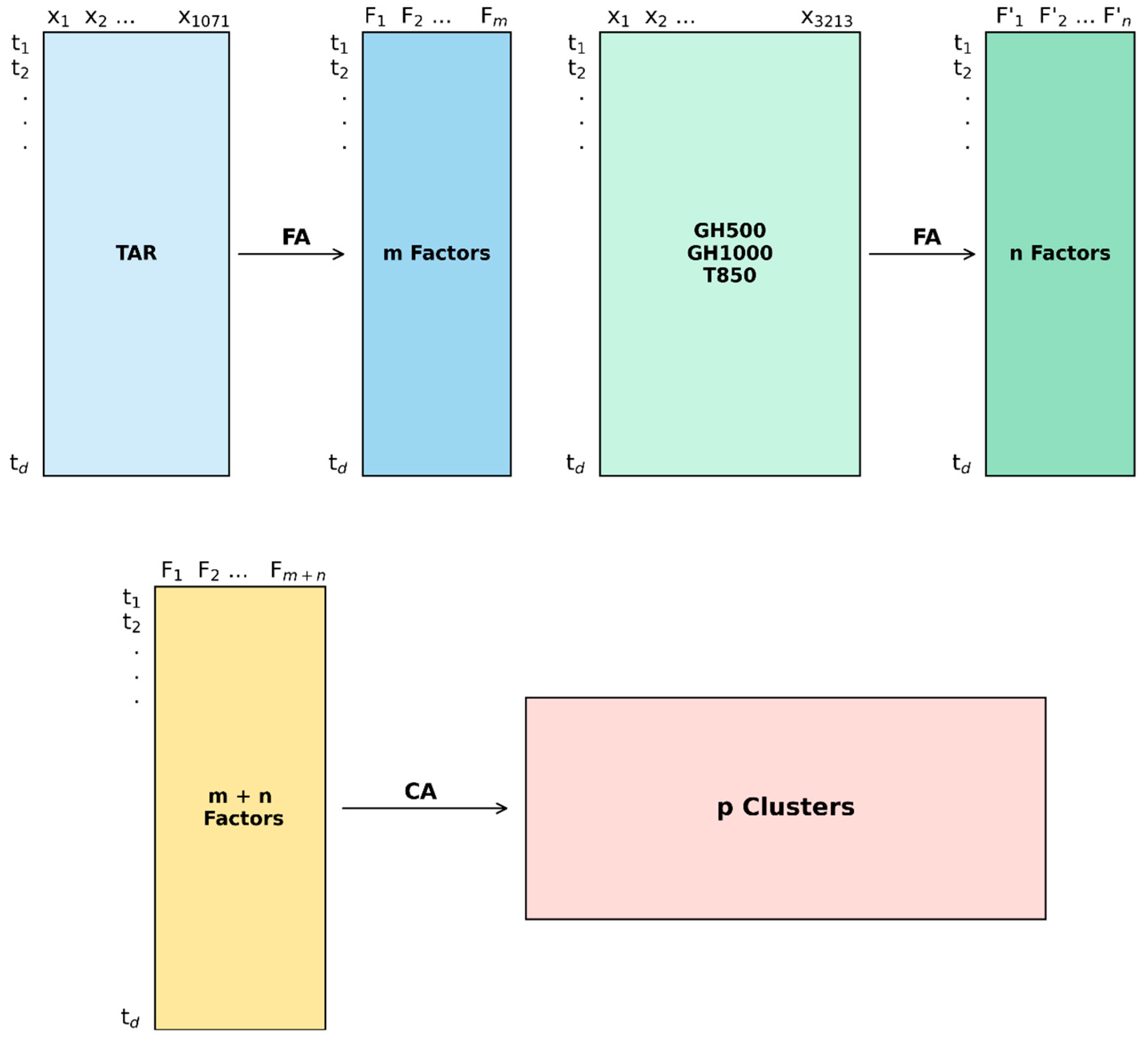
2.2. Methodology
3. Results and Discussion
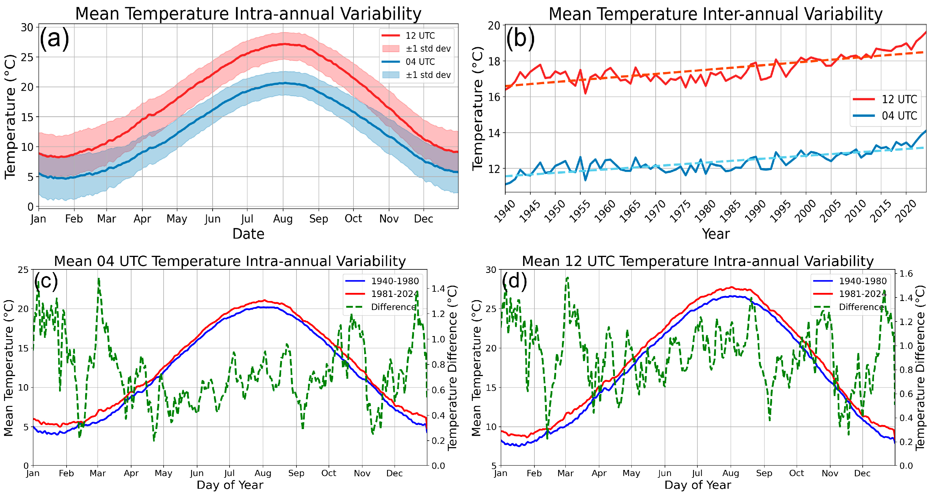
3.1. Temperature Statistics
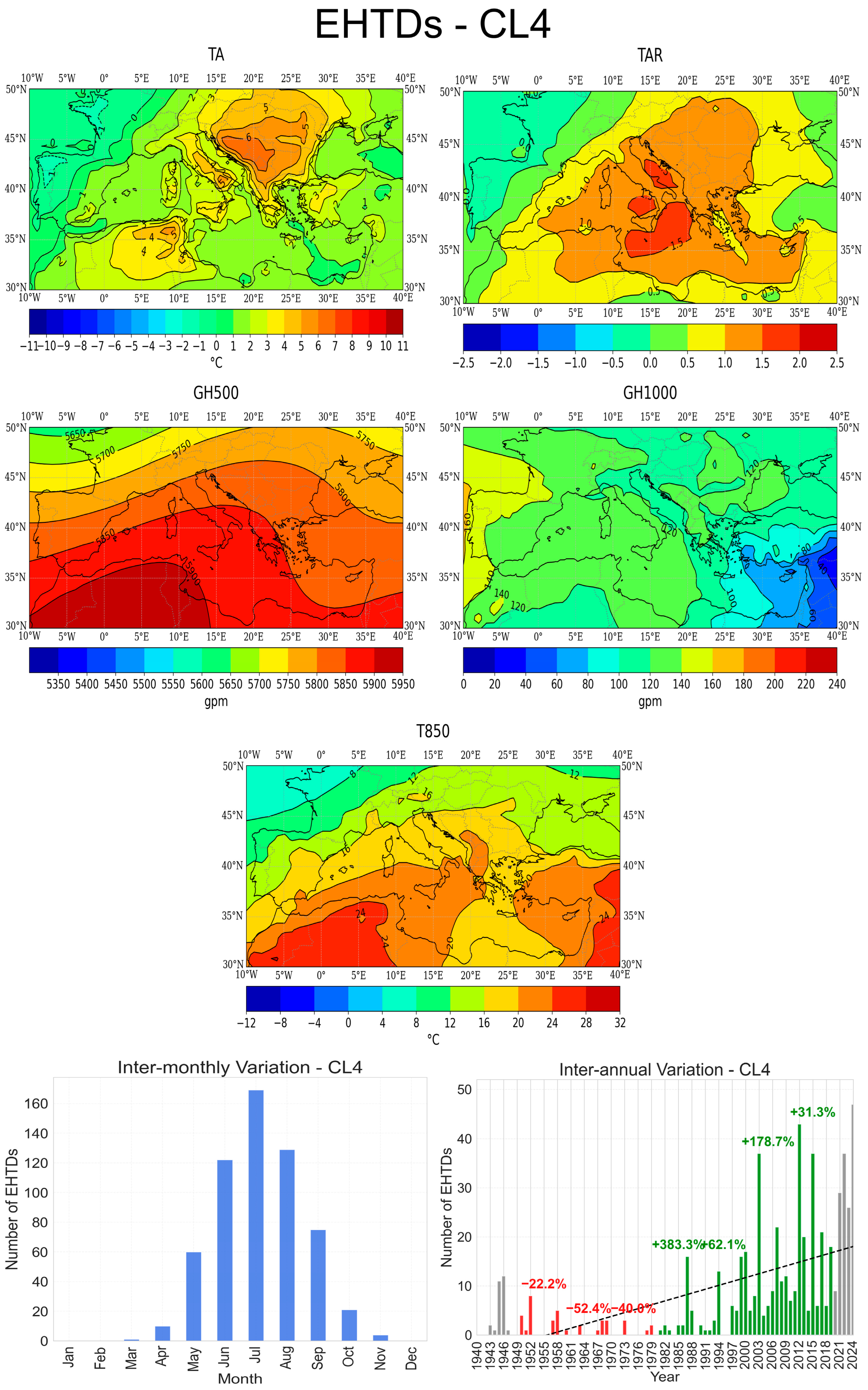
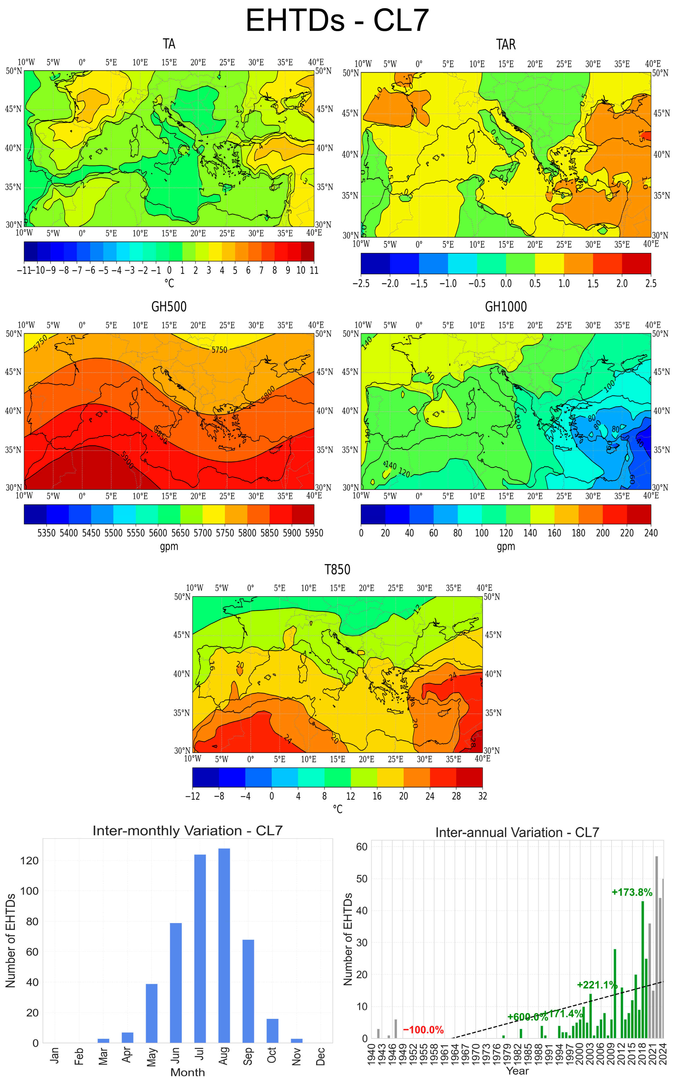
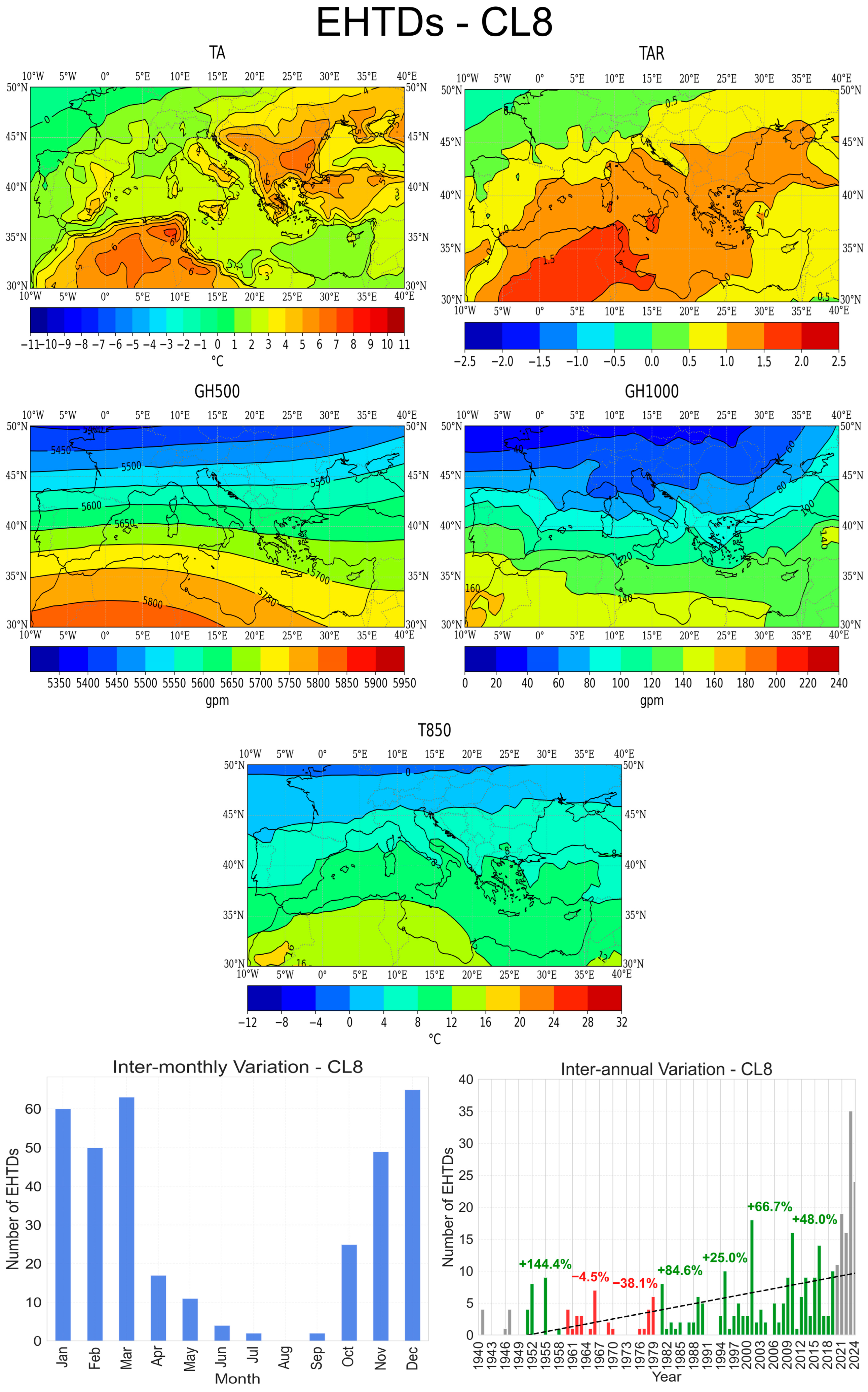
3.2. EHTDs
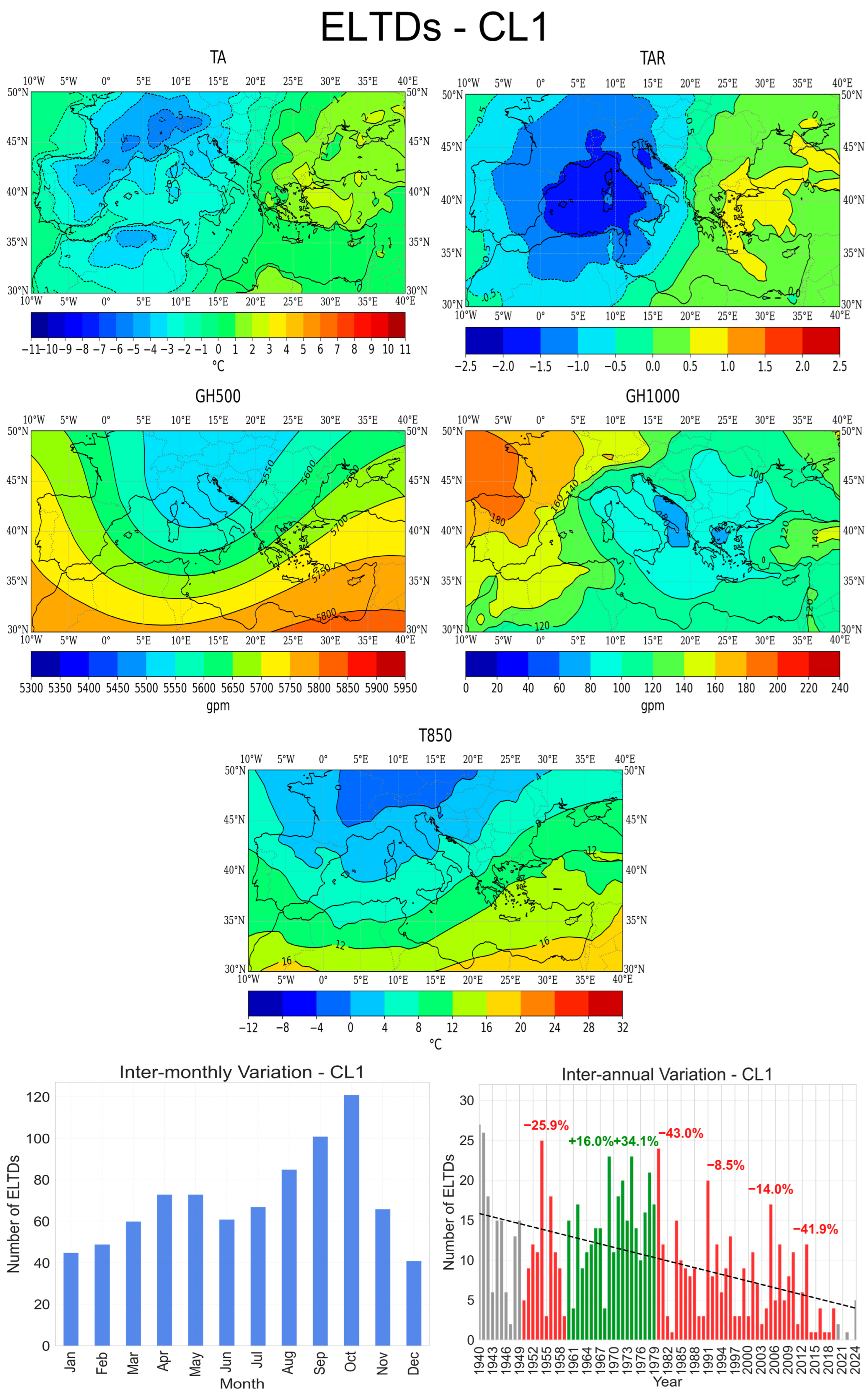
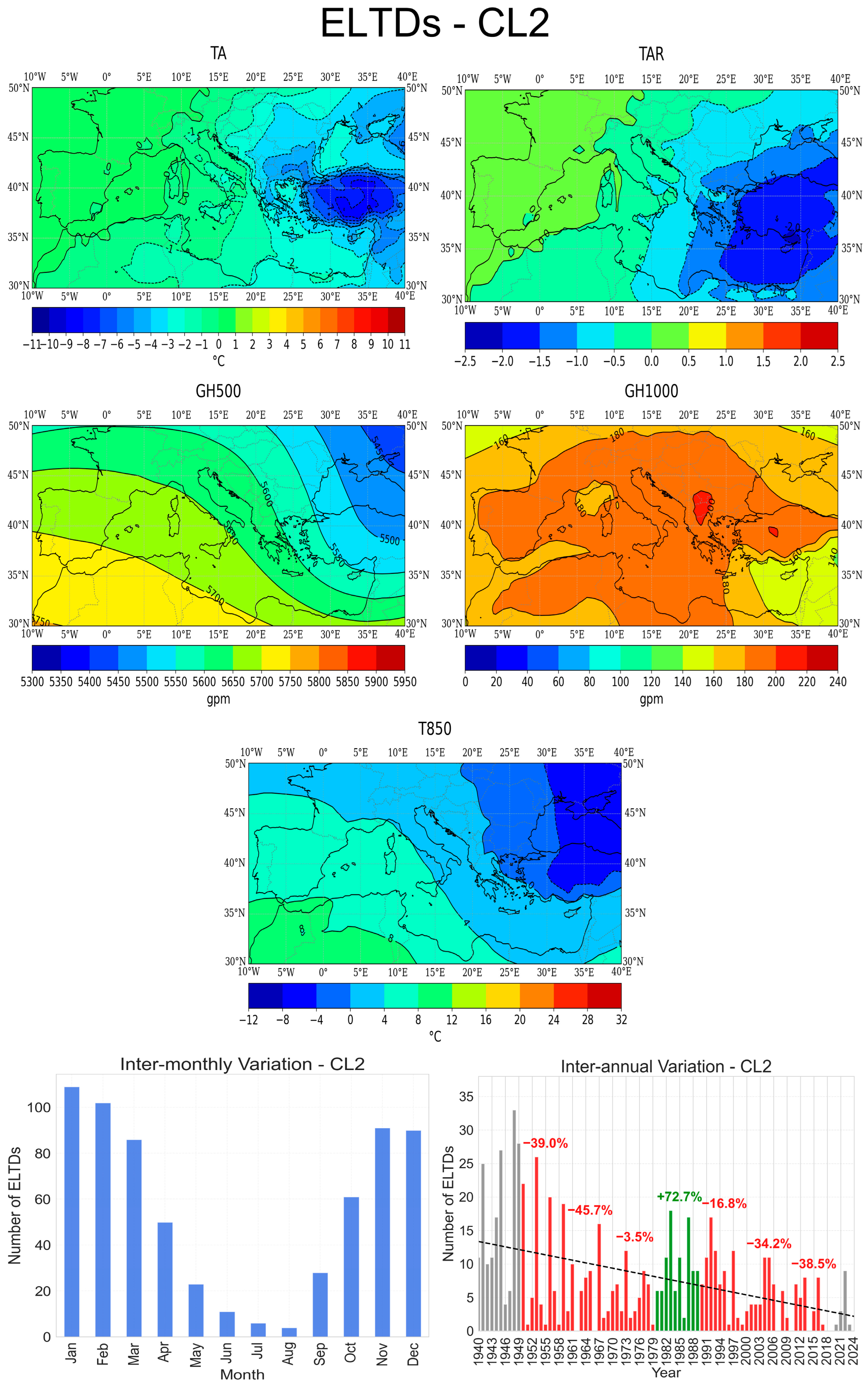
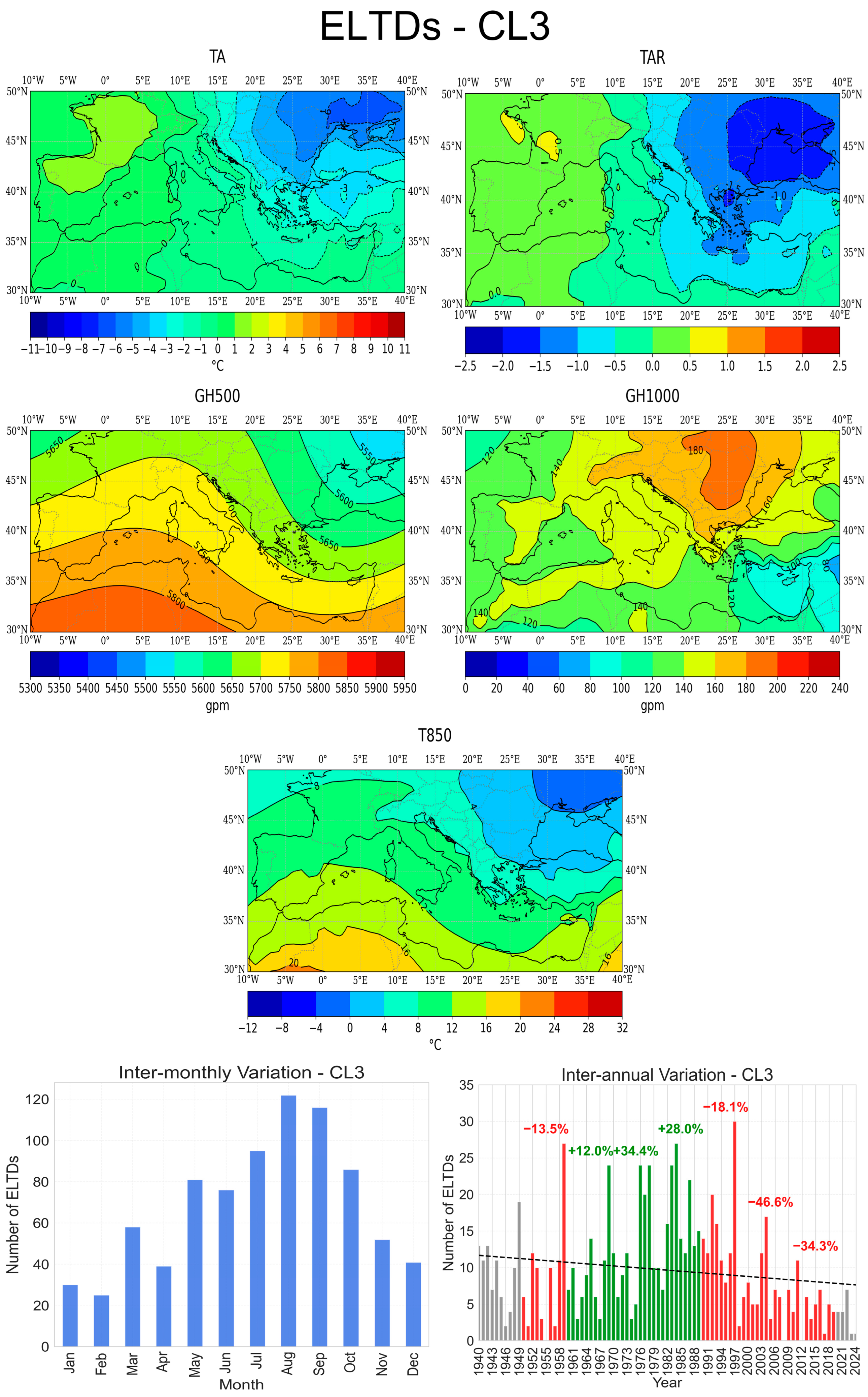
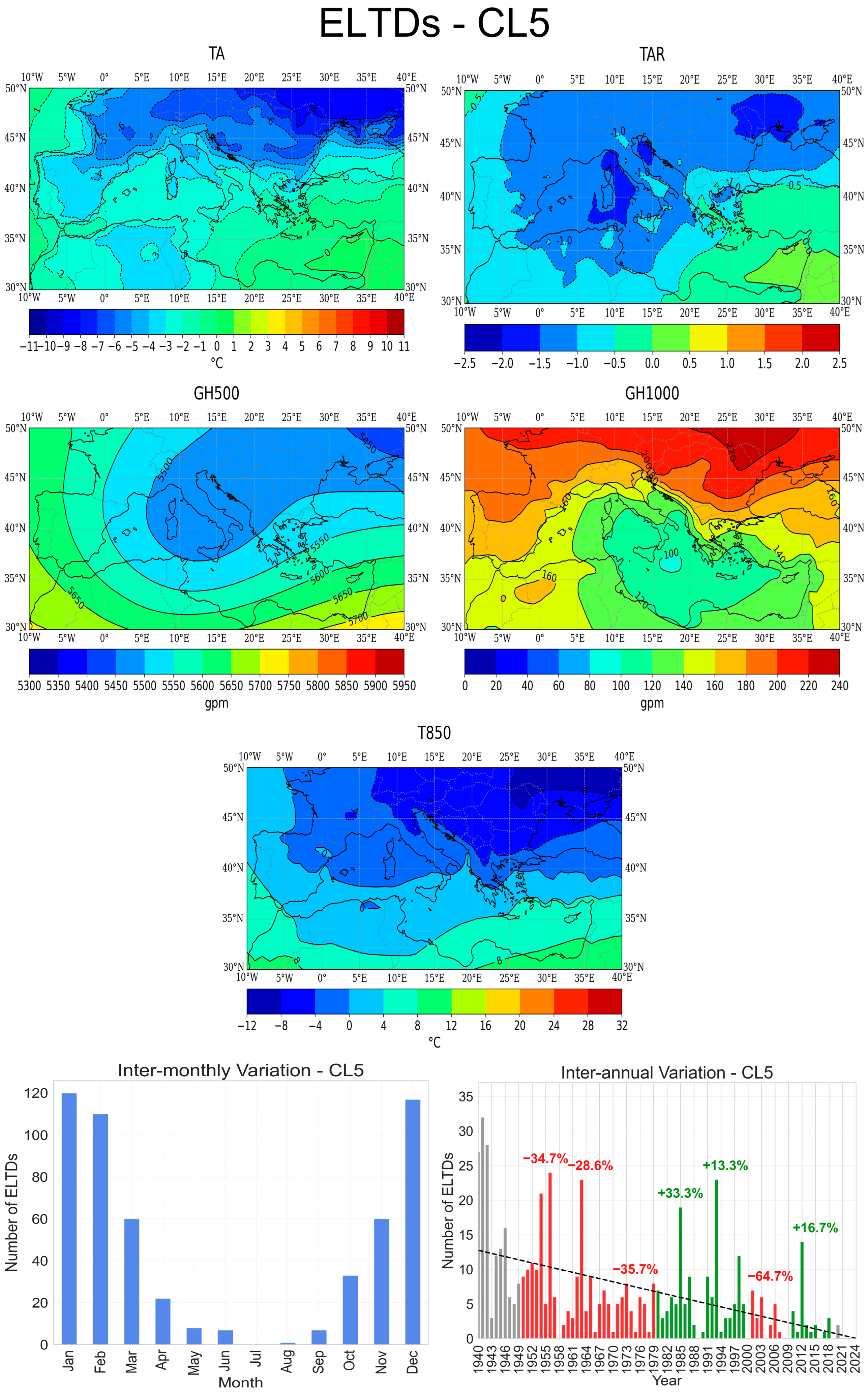
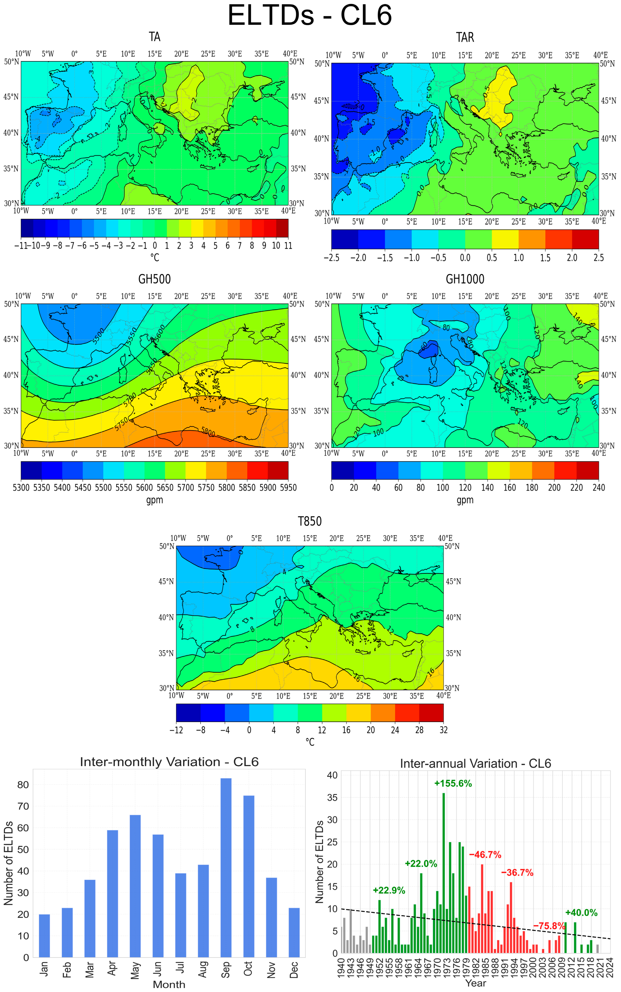
3.3. ELTDs
4. Conclusions
- A clear intensification of temperature extremes was found. EHTDs display a significantly increased frequency, while ELTDs have significantly decreased, especially during the 21st century. These tendencies highlight a shifting of the temperature regime in the Mediterranean and are consistent with the regional warming trends linked to climate change.
- Distinct circulation patterns were associated with each type of extreme. EHTDs typically occur under strong anticyclonic conditions, promoting blocking, solar heating and warm advection. ELTDs are associated with radiative cooling, cold advection and polar air mass intrusions. This connection between extremes and synoptic-scale atmospheric circulation conditions provides new insight into the mechanisms behind Mediterranean temperature extremes.
- Seasonal differences were revealed. Warm period EHTDs are dominated by mid-tropospheric ridges leading to the occurrence of heatwaves, while cold period EHTDs involve atmospheric blocking systems favoring the development of heat domes. On the other hand, warm period ELTDs are characterized by persistent surface cyclonic systems resulting in cold air advection, while cold period ELTDs are associated with blocking highs favoring radiative cooling and polar air mass intrusions.
- A high contrast in the occurrence between the extremes over land and sea was shown. This is highlighted by the effect of daytime radiative warming (peaking during summer for EHTDs) and the nighttime radiative cooling (peaking during winter for ELTDs) which are overlapping with the impact of warm and cold air advection leading to the appearance of extreme temperature days.
- All present findings, especially the remarkable statistically significant positive/negative trends in the number of ETHDs/ELTDs, are in agreement with the recent warming of the Mediterranean climate attributed to ongoing climate change [5,43]. Compared with earlier studies, this work utilizes long-term high spatiotemporal resolution reanalysis data covering the entire Mediterranean region for clustering temperature extremes with the associated synoptic patterns, therefore filling a key knowledge gap and improving the robustness and spatial relevance of temperature extreme classifications.
- Applying the current clustering methodology to compound events like heatwaves with drought by utilizing 2 m temperature and precipitation anomalies and involving local-scale observations and downscaled model data.
- Investigating the connection between temperature extremes and large-scale atmospheric oscillations (NAO, AO, EA-WR) using correlation and composite analysis techniques to improve forecasting capabilities and assist in the development of early warning strategies for Mediterranean climate extremes.
Author Contributions
Funding
Institutional Review Board Statement
Informed Consent Statement
Data Availability Statement
Acknowledgments
Conflicts of Interest
References
- IPCC 2023: Climate Change 2023 Synthesis Report; Contribution of Working Groups I, II and III to the Sixth Assessment Report of the Intergovernmental Panel on Climate Change; Core Writing Team, Lee, H., Romero, J., Eds.; IPCC: Geneva, Switzerland, 2023; pp. 35–115. [Google Scholar] [CrossRef]
- Frame, D.J.; Rosier, S.M.; Noy, I.; Harrington, L.J.; Carey-Smith, T.; Sparrow, S.N.; Stone, D.A.; Dean, S.M. Climate change attribution and the economic costs of extreme weather events: A study on damages from extreme rainfall and drought. Clim. Change 2020, 16, 781–797. [Google Scholar] [CrossRef]
- Van Garderen, L.; Feser, F.; Shepherd, T.G. A methodology for attributing the role of climate change in extreme events: A global spectrally nudged storyline. Nat. Hazards Earth Syst. 2021, 21, 171–186. [Google Scholar] [CrossRef]
- Cramer, W.; Guiot, J.; Fader, M.; Garrabou, J.; Gattuso, J.-P.; Iglesias, A.; Lange, M.A.; Lionello, P.; Llasat, M.C.; Paz, S.; et al. Climate change and interconnected risks to sustainable development in the Mediterranean. Nat. Clim. Change 2018, 8, 972–980. [Google Scholar] [CrossRef]
- MedECC. Climate and Environmental Change in the Mediterranean Basin—Current Situation and Risks for the Future. First Mediterranean Assessment Report; Cramer, W., Guiot, J., Marini, K., Eds.; Union for the Mediterranean, Plan Bleu, UNEP/MAP: Marseille, France, 2020; 632p. [Google Scholar] [CrossRef]
- Tuel, A.; Eltahir, E.A.B. Why Is the Mediterranean a Climate Change Hot Spot? J. Clim. 2020, 33, 5829–5843. [Google Scholar] [CrossRef]
- Xoplaki, E.; Luterbacher, J.; Paeth, H.; Dietrich, D.; Steiner, N.; Grosjean, M.; Wanner, H. European spring and autumn temperature variability and change of extremes over the last half millennium. Geophys. Res. Lett. 2005, 32, L15713. [Google Scholar] [CrossRef]
- Hertig, E.; Seubert, S.; Jacobeit, J. Temperature extremes in the Mediterranean area: Trends in the past and assessments for the future. Nat. Hazards Earth Syst. Sci. 2010, 10, 2039–2050. [Google Scholar] [CrossRef]
- Efthymiadis, D.; Goodess, C.M.; Jones, P.D. Trends in Mediterranean gridded temperature extremes and large-scale circulation influences. Nat. Hazards Earth Syst. Sci. 2011, 11, 2199–2214. [Google Scholar] [CrossRef]
- Lionello, P.; Scarascia, L. The relation of climate extremes with global warming in the Mediterranean region and its north versus south contrast. Reg. Environ. Change 2020, 20, 31. [Google Scholar] [CrossRef]
- Lolis, C.J.; Kotsias, G.; Farmakidis, D. A 40-year climatology of air temperature extremes in the southern Balkans based on the ERA5 database. Theor. Appl. Climatol. 2022, 149, 355–377. [Google Scholar] [CrossRef]
- Zittis, G.; Almazroui, M.; Alpert, P.; Ciais, P.; Cramer, W.; Dahdal, Y.; Fnais, M.; Francis, D.; Hadjinicolaou, P.; Howari, F.; et al. Climate Change and Weather Extremes in the Eastern Mediterranean and Middle East. Rev. Geophys. 2022, 60, e2021RG000762. [Google Scholar] [CrossRef]
- Bağçaci, S.Ç.; Yucel, I.; Duzenli, E.; Yilmaz, M.T. Intercomparison of the expected change in the temperature and the precipitation retrieved from CMIP6 and CMIP5 climate projections: A Mediterranean hot spot case, Turkey. Atmos. Res. 2021, 256, 105576. [Google Scholar] [CrossRef]
- Lorenzo, N.; Díaz-Poso, A.; Royé, D. Heatwave intensity on the Iberian Peninsula: Future climate projections. Atmos. Res. 2021, 258, 105655. [Google Scholar] [CrossRef]
- Ntoumos, A.; Hadjinicolaou, P.; Zittis, G.; Lelieveld, J. Updated Assessment of Temperature Extremes over the Middle East–North Africa (MENA) Region from Observational and CMIP5 Data. Atmosphere 2020, 11, 813. [Google Scholar] [CrossRef]
- Papadopoulos, G.; Keppas, S.C.; Parliari, D.; Kontos, S.; Papadogiannaki, S.; Melas, D. Future Projections of Heat Waves and Associated Mortality Risk in a Coastal Mediterranean City. Sustainability 2024, 16, 1072. [Google Scholar] [CrossRef]
- Hersbach, H.; Bell, B.; Berrisford, P.; Hiraharaet, S.; Horányi, A.; Muñoz-Sabater, J.; Nicolas, J.; Peubey, C.; Radu, R.; Schepers, D.; et al. The ERA5 global reanalysis. Q. J. R. Meteorol. Soc. 2020, 146, 1999–2049. [Google Scholar] [CrossRef]
- Korhonen, N.; Hyvärinen, O.; Kollanus, V.; Lanki, T.; Jokisalo, J.; Kosonen, R.; Richardson, D.S.; Jylhä, K. The probabilistic skill of extended-range heat wave forecasts over Europe. Nat. Hazards Earth Syst. Sci. 2025, 25, 1865–1879. [Google Scholar] [CrossRef]
- Jiang, N.; Cheung, K.; Luo, K.; Beggs, P.J.; Zhou, W. On two different objective procedures for classifying synoptic weather types over east Australia. Int. J. Climatol. 2012, 32, 1475–1494. [Google Scholar] [CrossRef]
- Kotsias, G.; Lolis, C.J.; Hatzianastassiou, N.; Lionello, P.; Bartzokas, A. A comparison of different approaches for the definition of seasons in the Mediterranean region. Int. J. Climatol. 2021, 42, 1954–1974. [Google Scholar] [CrossRef]
- Lin, S.; Wei, K.; Lei, Q.; Shao, F.; Wang, Q.; Deng, M.; Su, L. Identification and prediction of climate factors based on factor analysis and a grey prediction model in China. Environ. Monit. Assess. 2023, 195, 751. [Google Scholar] [CrossRef]
- Jolliffe, I.T. Principal Component Analysis; Springer: New York, NY, USA, 1986. [Google Scholar]
- Richman, M.B. Rotation of principal components. Int. J. Climatol. 1986, 6, 293–335. [Google Scholar] [CrossRef]
- Wong, M.A.; Hartigan, J.A. Algorithm AS 136: A k-means clustering algorithm. J. R. Stat. Soc. Ser. C Appl. Stat. 1979, 28, 100–108. [Google Scholar]
- Sharma, S. Applied Multivariate Techniques; Wiley: New York, NY, USA, 1995. [Google Scholar]
- Sugar, A.C.; James, M.G. Finding the number of clusters in a dataset: An information–theoretic approach. J. Am. Stat. Assoc. 2003, 98, 750–763. [Google Scholar] [CrossRef]
- Kendall, M. Multivariate Analysis; Charles Griffin: London, UK, 1975; p. 210. [Google Scholar]
- Di Bernardino, A.; Casadio, S.; Iannarelli, A.M.; Siani, A.M. Temperature Trends and Influence of the Base Period Selection on Climate Indices in the Mediterranean Region over the Period 1961–2020. Int. J. Climatol. 2024, 44, 5969–5985. [Google Scholar] [CrossRef]
- Zhang, X.; Zhou, T.; Zhang, W.; Zhu, C.; Yang, F.; Li, C.; Gao, J.; Sun, Y. Increased impact of heat domes on 2021-like heat extremes in North America under global warming. Nat. Commun. 2023, 14, 1690. [Google Scholar] [CrossRef]
- Tomczyk, A.M.; Bednorz, E. Heat waves in Central Europe and their circulation conditions. Int. J. Climatol. 2016, 36, 770–782. [Google Scholar] [CrossRef]
- Kostopoulou, E.; Jones, P. Assessment of climate extremes in the Eastern Mediterranean. Meteorol. Atmos. Phys. 2005, 89, 69–85. [Google Scholar] [CrossRef]
- Tyrlis, E.; Lelieveld, J. Climatology and dynamics of the summer Etesian winds over the eastern Mediterranean. J. Atmos. Sci. 2013, 70, 3374–3396. [Google Scholar] [CrossRef]
- Tomczyk, A.M.; Półrolniczak, M.; Bednorz, E. Circulation conditions’ effect on the occurrence of heat waves in Western and Southwestern Europe. Atmosphere 2017, 8, 31. [Google Scholar] [CrossRef]
- Hochman, A.; Marra, F.; Messori, G.; Pinto, J.G.; Raveh-Rubin, S.; Yosef, Y.; Zittis, G. Extreme weather and societal impacts in the eastern Mediterranean. Earth Syst. Dynam. 2022, 13, 749–777. [Google Scholar] [CrossRef]
- Zhang, X.; Aguilar, E.; Sensoy, S.; Melkonyan, H.; Tagiyeva, U.; Ahmed, N.; Kutaladze, N.; Rahimzadeh, F.; Taghipour, F.; Hantosh, T.H.; et al. Trends in Middle East climate extreme indices from 1950 to 2003. J. Geophys. Res. 2005, 110, D22104. [Google Scholar] [CrossRef]
- D’Errico, M.; Pons, F.; Yiou, P.; Tao, S.; Nardini, C.; Lunkeit, F.; Faranda, D. Present and future synoptic circulation patterns associated with cold and snowy spells over Italy. Earth Syst. Dynam. 2022, 13, 961–992. [Google Scholar] [CrossRef]
- Nygård, T.; Papritz, L.; Naakka, T.; Vihma, T. Cold wintertime air masses over Europe: Where do they come from and how do they form? Weather Clim. Dynam. 2023, 4, 943–961. [Google Scholar] [CrossRef]
- Tringa, E.; Tolika, K.; Anagnostopoulou, C.; Kostopoulou, E. A Climatological and Synoptic Analysis of Winter Cold Spells over the Balkan Peninsula. Atmosphere 2022, 13, 1851. [Google Scholar] [CrossRef]
- Trigo, R.M.; Trigo, I.F.; DaCamara, C.C.; Osborn, T.J. Climate impact of the European winter blocking episodes from the NCEP/NCAR Reanalyses. Clim. Dyn. 2004, 23, 17–28. [Google Scholar] [CrossRef]
- Brunet, M.; Jones, P.D.; Sigró, J.; Saladié, O.; Aguilar, E.; Moberg, A.; Della-Marta, P.M.; Lister, D.; Walther, A.; López, D. Temporal and spatial temperature variability and change over Spain during 1850–2005. J. Geophys. Res. 2007, 112, D12117. [Google Scholar] [CrossRef]
- Bartolini, G.; Morabito, M.; Crisci, A.; Grifoni, D.; Torrigiani, T.; Petralli, M.; Maracchi, G.; Orlandini, S. Recent trends in Tuscany (Italy) summer temperature and indices of extremes. Int. J. Climatol. 2008, 28, 1751–1760. [Google Scholar] [CrossRef]
- Kuglitsch, F.G.; Toreti, A.; Xoplaki, E.; Della-Marta, P.M.; Zerefos, C.; Türkes¸, M.; Luterbacher, J. Heat wave changes in the eastern Mediterranean since 1960. Geophys. Res. Lett. 2010, 37, L0482. [Google Scholar] [CrossRef]
- Knobler, S.; Rilov, G.; Garfinkel, C.I.; Liberzon, D. Climate change impacts in Eastern Mediterranean Sea: Trends and extremes. Water Waves 2025. [Google Scholar] [CrossRef]
- Zveryaev, I.I.; Arkhipkin, A.V. Structure of climatic variability of the Mediterranean sea surface temperature, Part, I. Standard deviations and linear trends. Russ. Meteorol. Hydrol. 2008, 33, 377–382. [Google Scholar] [CrossRef]
- Zveryaev, I.I.; Arkhipkin, A.V. Structure of climatic variability of the Mediterranean sea surface temperature, Part II. Principal modes of variability. Russ. Meteorol. Hydrol. 2008, 33, 446–452. [Google Scholar] [CrossRef]


| CL | Intra-Annual Frequency | Main Affected Areas—High TA/TAR Values | Synoptic Pattern and Features |
|---|---|---|---|
| CL1 | Cold period, max in spring | W Mediterranean (Iberian Peninsula, Algeria) | Surface anticyclone, 500 hPa ridge, high T850; heat dome |
| CL2 | Cold period, max in winter | Continental Europe | Surface anticyclone, 500 hPa ridge; blocking system |
| CL3 | Year-round, min in winter | E Mediterranean (Balkans, Middle East) | Depression and anticyclone combination; warm air advection |
| CL4 | Summer | Mediterranean Sea axis, Balkans, North Africa | Strong 500 hPa ridge, high T850; heat dome |
| CL5 | Warm period | Central and western Europe | Surface anticyclone, 500 hPa ridge; prolonged heatwaves |
| CL6 | Cold period, max in spring | E Mediterranean (NE Africa, Greece, Middle East) | Surface depression, high T850; warm air advection |
| CL7 | Summer | Entire Mediterranean, highest in E Mediterranean and W Europe | Surface anticyclone, 500 hPa ridge, high T850; warm air advection |
| CL8 | Cold period | NW Africa, central and western Mediterranean, Balkans | Parallel GH500 and GH1000 isopleths; strong westerlies, heat dome |
| CL9 | Cold period | Central Mediterranean, Balkans | Surface cyclone—anticyclone combination, 500 hPa ridge, high T850; warm air advection |
| CL | Intra-Annual Frequency | Main Affected Areas—High TA/TAR Values | Synoptic Pattern and Features |
|---|---|---|---|
| CL1 | All-year-round | Central and western Mediterranean | Cyclone–anticyclone combination; cold air advection |
| CL2 | Cold period | E Mediterranean and Middle East | Surface anticyclone, low T850; blocking system, radiative cooling |
| CL3 | Warm period | E Europe | Surface anticyclone, low T850; cold advection, temperature inversions |
| CL4 | All-year-round | Central and eastern Mediterranean (Italy, Greece, Balkans) | Cyclone–anticyclone combination, deep 500 hPa trough; cold advection, polar air mass intrusions |
| CL5 | Cold period | Continental Europe and central/western Mediterranean | Surface blocking anticyclone, 500 hPa trough; cold air advection, radiative cooling |
| CL6 | Warm period | W Mediterranean | Surface cyclone, 500 hPa trough, low T850; cold air advection |
| CL7 | Cold period | N Europe | 500 hPa trough, low T850; Arctic outbreaks, polar vortex disruptions |
Disclaimer/Publisher’s Note: The statements, opinions and data contained in all publications are solely those of the individual author(s) and contributor(s) and not of MDPI and/or the editor(s). MDPI and/or the editor(s) disclaim responsibility for any injury to people or property resulting from any ideas, methods, instructions or products referred to in the content. |
© 2025 by the authors. Licensee MDPI, Basel, Switzerland. This article is an open access article distributed under the terms and conditions of the Creative Commons Attribution (CC BY) license (https://creativecommons.org/licenses/by/4.0/).
Share and Cite
Kotsias, G.; Lolis, C.J. Air Temperature Extremes in the Mediterranean Region (1940–2024): Synoptic Patterns and Trends. Atmosphere 2025, 16, 852. https://doi.org/10.3390/atmos16070852
Kotsias G, Lolis CJ. Air Temperature Extremes in the Mediterranean Region (1940–2024): Synoptic Patterns and Trends. Atmosphere. 2025; 16(7):852. https://doi.org/10.3390/atmos16070852
Chicago/Turabian StyleKotsias, Georgios, and Christos J. Lolis. 2025. "Air Temperature Extremes in the Mediterranean Region (1940–2024): Synoptic Patterns and Trends" Atmosphere 16, no. 7: 852. https://doi.org/10.3390/atmos16070852
APA StyleKotsias, G., & Lolis, C. J. (2025). Air Temperature Extremes in the Mediterranean Region (1940–2024): Synoptic Patterns and Trends. Atmosphere, 16(7), 852. https://doi.org/10.3390/atmos16070852