Comparative Analysis of Machine Learning Algorithms for Potential Evapotranspiration Estimation Using Limited Data at a High-Altitude Mediterranean Forest

Abstract

Accurate estimation of potential evapotranspiration (PET) is of paramount importance for water resource management, especially in Mediterranean mountainous environments that are often data-scarce and highly sensitive to climate variability. This study evaluates the performance of four machine learning (ML) regression algorithms—Support Vector Regression (SVR), Random Forest Regression (RFR), Gradient Boosting Regression (GBR), and K-Nearest Neighbors (KNN)—in predicting daily PET using limited meteorological data from a high-altitude in Central Greece. The ML models were trained and tested using easily available meteorological inputs—temperature, relative humidity, and extraterrestrial solar radiation—on a dataset covering 11 years (2012–2023). Among the tested configurations, RFR showed the best performance (R² = 0.917, RMSE = 0.468 mm/d, MAPE = 0.119 mm/d) when all the above-mentioned input variables were included, closely approximating FAO56–PM outputs. Results bring to light the potential of machine learning models to reliably estimate PET in data-scarce conditions, with RFR outperforming others, whereas the inclusion of the easily estimated extraterrestrial radiation parameter in the ML models training enhances PET prediction accuracy.

1. Introduction

Evapotranspiration (ET) is a fundamental physical process that shapes and sustains ecosystems, influences weather and climate patterns, and mediates the exchange of water and energy between the land surface and atmosphere. It directly affects vegetation water requirements and plays a crucial role across various geoscience disciplines, including hydrology, climatology, ecology, agriculture, and forestry. In the context of climate change rising temperatures, land use, solar radiation changes, and shifts in precipitation patterns significantly influence actual ET trends [1,2]. Future climate projections foresee increased ET and potential evapotranspiration (PET) fluxes, exacerbating aridity, and intensifying water-related stress in Mediterranean ecosystems [3]. This trend underscores the urgency of improving ET estimation accuracy, particularly in regions where water availability is already under pressure due to climate variability. This increasing variability highlights the urgent need to improve ET estimation accuracy, especially in regions already experiencing water scarcity.

Therefore, precise ET and PET estimates are essential for sustainable water resource management and climate adaptation strategies. Direct measurements of ET using lysimeters [4,5] or the eddy covariance technique [6,7] are the most accurate methods to monitor the actual fluxes, with limited assumptions [8], offering valuable insights into ecosystem-scale actual ET dynamics under specific vegetation and climate conditions. Nevertheless, such methods are often challenging and, in many cases, infeasible due to the high costs of the installation and maintenance of the necessary equipment. To that end, the use of the PET is easier to apply for monitoring the atmospheric water demand. Several empirical mathematical models based on different physical and conceptual basis, have been developed globally across different environmental conditions for its estimation [9]. These models rely on meteorological data measured by ground stations installed above natural surfaces, demonstrating that the site’s surface characteristics highly influence the PET rates [10]. Designed to estimate water demand based on atmospheric conditions, empirical PET models minimize the impact of plant species, vegetation phenology, or soil properties. However, these factors are indirectly reflected in the meteorological attributes measured at each site, particularly temperature and humidity, which both influence and are influenced by evapotranspiration rates [10]. These models range from simple temperature-based equations to more complex ones that incorporate multiple meteorological variables. Generally, they can be classified into four major categories: according to their requirements for input parameters: mass transfer methods, temperature-based methods, radiation-based methods, and combination methods. In the literature, more than one hundred models have been identified, many of which provide reliable results [10]. Considering that the proposed PET methods are site-specific and present both spatial and temporal variability, the selection of the appropriate method for each area is crucial and, in most cases, requires adjustment in order to produce accurate assessments of dryness, aridity, identification of hydrometeorological extremes, or other water related attributes for climate classification [11,12,13].

The Food and Agriculture Organization (FAO) and World Meteorological Organization (WMO) recommend the FAO56 Penman–Monteith (FAO56–PM) model for estimating PET [14], acknowledging its robustness across diverse climates and conditions. Given its inclusion of physiological and aerodynamic criteria, which eliminates the need for local calibration and so provides a consistent approach for PET, this model has become the global benchmark. Furthermore, the FAO56–PM method has been validated against lysimeter data, underscoring its reliability [15,16]. However, its extensive data requirements, including air temperature, relative humidity, net radiation, wind speed, atmospheric pressure, and soil heat flux, measured above reference surfaces can restrict its application in regions lacking complete meteorological stations or high-quality data collection facilities. Notably, the cost of collecting this data is relatively high not only in developed countries, but also, and most particularly, in developing countries [17]. Along with the required technical support, the financial load of acquiring, installing, and maintaining specialized agrometeorological equipment—including pyranometers, anemometers, hygrometers, and barometers—can be very significant. This economic restriction frequently results in data gaps since it lacks resources to sustain continuous and high-quality data collecting infrastructure over several years [18,19,20]. It should be also noted that many of the input parameters of the FAO56-PM are measured by the ground stations only during the last decades, whereas longer time series of historical meteorological data include only a small variety of measured parameters (mainly air temperature and precipitation). Under this view, the application of the FAO56–PM is restricted, and the long-period evaluation of PET fluxes would be prohibited. Thus, less data-intensive PET models, producing accurate PET estimates were necessary to be evaluated and adjusted to each site-specific condition. Moreover, even in cases of available equipment, obtaining reliable data for the application of FAO56-PM can be challenging due to issues including sensor malfunction risks, calibration requirements, and data quality control in remote or under-resourced settings [21]. To overcome these limitations, satellite-derived meteorological data became alternative sources for estimating PET over large areas using empirical models [22]. However, these approaches usually present uncertainties at finer spatial scales due to microclimatic variations [23,24].

During the last years, the usage of Machine Learning (ML) has emerged as a powerful tool for dealing with the complexities involved in PET estimation [25]. ML models provide flexibility; understanding complex patterns in a dataset and reducing dependence on comprehensive meteorological inputs [26]. They are proven to be efficient in processing varied meteorological variables such as temperature, relative humidity, radiation, and wind speed in predicting PET with high accuracy under different environmental conditions. Numerous studies have shown that ML techniques consistently outperform empirical or semi-empirical PET methods [27,28,29]. A novel approach by Ahmadi et al. [30] introduced “SolarET”, a ML approach-based method aimed at estimating daily PET using only solar radiation data. The results show that ML models provide better results compared with well-known methods such as Hargreaves–Samani [31], Romanenko [32] and Priestley–Taylor [33]. Even though the incoming solar radiation flux density (Rs) is the only meteorological variable that is not directly affected by the surface characteristics, it is often excluded from ML approaches for PET estimation due to the lack of long-term Rs time series data recorded by pyranometers.

To this end, scholars have employed ML models with a restricted set of variables, which are usually available through low-cost sensors. Key inputs to these models are routinely measured meteorological parameters including temperature and relative humidity. This strategy not only improves the feasibility of data collecting, but it also encourages the use of advanced analytical techniques in a variety of environmental settings. For instance, Ferreira et al. [34] compare the performance of Artificial Neural Networks (ANNs) and Support Vector Machines (SVMs) models in calculating PET across Brazil, utilizing average temperature and relative humidity data or temperature attributes (minimum, maximum, or mean temperature) solely. Both models showed reasonable accuracy, thereby demonstrating the potential of ML methods with few inputs. Similarly, Bellido-Jimenez et al. [35] explored ML methods—such as multilayer perceptron (MLP), generalized regression neural network (GRNN), extreme learning machine (ELM), SVM, and random forest (RF)—to estimate PET using only temperature data in southern Spain. They found that ML models exhibit comparable performance with the FAO56–PM method and outperform empirical models. In Pakistan, Mostafa et al. [36] compare the efficiency of random vector functional link (RVFL) and relevance vector machine (RVM) algorithms in PET estimation. In their approach, they use temperature data (minimum and maximum temperatures) and extraterrestrial radiation (Ra), which is estimated by using the station’s location, specifically its latitude and day of the year. Finally, a comprehensive study was conducted by Diamantopoulou and Papamichail [37] on the usage of ML models for PET estimation based on temperature (mean, maximum, and minimum components). Several regression-based models were tested, like Support Vector Regression (SVR), RF, and GRNN, and found that SVR approximates better FAO56–PM values, while all ML models provide better accuracy than the empirical methods.

The authors are not aware of any studies that have trained and evaluated the performance of ML models for PET estimation at high-altitude Mediterranean sites. This is due to the challenges in installing and maintaining meteorological sensors, especially in mountainous areas. In most cases, data from plain or semi-mountainous sites are used for the ML model’s development, and thus, the results cannot be exploited to crucial mountainous forest ecosystems. These ecosystems are vital, as mountainous areas host a variety of important plant species and communities that are highly sensitive to water availability. This study aims to evaluate the performance of four ML regressor algorithms including SVR, RFR, Gradient Boosting (GBR), and KNeighbors (KNN) algorithms for PET estimation, at a high-altitude Mediterranean forest. Specific objectives are (i) compare ML-derived PET estimates with the benchmark FAO56–PM model, and (ii) identify the most effective combinations of input parameters to balance accuracy and data availability. The novelty of this study lies in evaluating the application of ML models in a high-altitude Mediterranean forest, where PET estimation is complicated by topographic influences and limited meteorological inputs, which can be acquired with a single thermohygrometer sensor, often standard in meteorological stations. Unlike pyranometers or other costly instruments, this approach minimizes technical and economic constraints. Additionally, this research examines the effectiveness of using extraterrestrial solar radiation—a parameter derived from geographic latitude—as a cost-effective alternative to traditional radiation measurements. By demonstrating the feasibility of low-input ML models under these conditions, this study contributes to improving PET estimation methodologies in mountainous, data-scarce regions. Ultimately, it supports climate adaptation and water resource management in these vulnerable ecosystems while paving the way for accessible, low-cost environmental monitoring systems.

2. Materials and Methods

2.1. Study Area

This research was conducted in the Pertouli forest, located within the Pindus Mountain range in Central Greece. This forest has been granted to the Aristotle University of Thessaloniki for research and educational purposes since 1934 and is managed by the University Forests Administration and Management Fund (UFAMF). To that end, it is labeled as University Forest. The forest site’s locations are illustrated in Figure 1.

The University Forest of Pertouli covers an area of 3290 hectares. The forest predominantly comprises pure fir stands (Abies borisii regis) and extends across elevations ranging from 1100 to 2073 m above sea level (m, a.s.l). The area belongs to the European environmental protection network known as Natura 2000 and has been specifically designated as a Site of Community Importance (SCI) with the code GR1440002, referred to as “Kerketio Oros (Koziakas)”. The following habitat types, as listed in Annex I of Directive 92/43/EEC, are present within this SCI: Alpine rivers and their ligneous vegetation with Salix elaeagnos (3240), Alpine and subalpine calcareous grasslands (6170), Lowland hay meadows (Alopecurus pratensis, Sanguisorba officinalis) (6510), Eastern Mediterranean screes (8140), Calcareous rocky slopes with chasmophytic vegetation (8210), and Hellenic beech forests with Abies borisii-regis (9270). The climate is characterized as a transitional Mediterranean mid-European climate, demonstrating cold, rainy winters contrasting with warm, dry summers. These distinctive climatic and environmental conditions create a challenging yet valuable setting for studying PET estimation using limited data. The combination of high-altitude Mediterranean features and the forest environment enhances the significance of this location for comparative analysis of machine learning algorithms in PET prediction.

Based on long-term temperature and precipitation data from the ground meteorological station operating in this site (altitude 1180 m a.s.l) since 1961, the pluviothermic diagram was created (Figure 2). A detailed description of the weather station can be also found in Stefanidis and Alexandridis [38].

The pluviothermic diagram clearly indicates a zero-length dry period in the site, attributed mainly to the relevantly high precipitation which on average reaches 1474 mm per year, distributed seasonally, by 37% in winter, 30% in autumn, and 24% in spring, being quite high also in summer (127 mm or 9% of the annual sum). The wettest month of the year is December (217 mm) and the driest is August (38 mm). The monthly air temperatures range from 0.1 °C in January to 18.9 °C in July, whereas the seasonal temperature pattern is anticipated for a Mediterranean climate, warmer in summer (18.0 °C) and cooler in winter (0.8 °C), with intermediate values in the transitional seasons of spring (7.8 °C) and autumn (9.9 °C). The annual air temperature for the site is 9.1 °C. The above pattern indicates that the vegetation water requirements (actual evapotranspiration) in the site, are generally covered by precipitation in all seasons. Thus, the potential evapotranspiration (PET) daily values are close to actual evapotranspiration, and the local vegetation is not likely to suffer from long-term interannual water shortages.

2.2. Meteorological Data and PET Estimates

An automated micrometeorological station was installed at the forest site to continuously monitor atmospheric conditions in close proximity with the manual ones. This station is located at latitude 39.54° N and longitude 21.46° E (1180 m a.s.l.) and operated by the Laboratory of Mountainous Water Management and Control of Aristotle University of Thessaloniki. It was equipped with precise sensors to measure key meteorological parameters. Wind speed and wind direction data were collected using the WindSonic sensor (1405-PK-040) from GILL INSTRUMENTS LTD, Lymington, UK, with an accuracy of ±2% and 30, respectively. For temperature and relative humidity measurements, the HD9817T.1 transmitter from DELTA OHM S.R.L., Caselle di Selvazzano Dentro, Padova, Italy, was utilized, providing precise readings with an accuracy of 0.20 °C and ±2%, respectively, along with a sensitivity change of 0.20 °C for temperature and 1% for relative humidity per year. Global and diffused radiation at wavelengths 400–2700 nm (accuracy ±5% daily integrals), as well as sunshine duration based on the threshold of 120 W m^–2 of WMO (±10% sun hours with respect to the threshold) are measured with the SPN1 Sunshine Pyranometer (DELTA-T DEVICES LTD, Cambridge, UK). The HD2013 Tipping Bucket Rain Gauge (Delta OHM, Caselle di Selvazzano Dentro, Padova, Italy) is used for precipitation measurements. The sensor measurement analysis is 0.2 mm and its accuracy 2%. The measurements were conducted every 5 s and the 10 min averages were recorded. The data available spans from 1 July 2012 to 22 June 2023. It is worth mentioning that the use of high precision sensors, in this work, is significant for the estimation of accurate PET daily fluxes.

The annual distribution of the main input parameters used in this work, during the recording, is presented in Figure 3. The monthly temperature ranged from 5.5 °C in winter to 17.9 °C, with moderate values (9.0 and 11.2 °C) in spring and autumn, which are higher compared to average climatic averages. Accordingly, the average minimum temperatures varied from 2.5 to 11.3 °C in summer, whereas the respective maximum temperatures were 9.1 and 25.7 °C. The relative humidity (RH) showed opposite distribution, with average, minimum, and maximum values ranging between 74.4, 45.2, and 96.0%, respectively, in summer to 88.6, 69.6, and 98.8% in winter, with annual values of 82.1%. The warmer conditions during the recording period, compared to the climatic pattern of the area, are also associated with wetter conditions, considering that the annual precipitation reached 1786 mm.

In this study, the performance of several machine learning algorithms is evaluated against the standardized FAO56 Penman–Monteith (FAO56–PM) method, which serves as the benchmark for estimating potential evapotranspiration (PET) [14]. The FAO56–PM equation is expressed as follows:

$$\mathrm{P}\mathrm{E}\mathrm{T}={\displaystyle \frac{0.408\Delta \left({\mathrm{R}}_{\mathrm{n}}-\mathrm{G}\right)+\mathsf{\gamma }\frac{900}{{\mathrm{T}}_{\mathrm{m}\mathrm{e}\mathrm{a}\mathrm{n}}+273}\mathrm{u}({\mathrm{e}}_{\mathrm{s}}-{\mathrm{e}}_{\mathrm{a}})}{\Delta +\mathsf{\gamma }\left(1+0.34\mathrm{u}\right)}}$$

(1)

where ${ET}_{P-M}$ is the potential evapotranspiration (mm/d), Δ is the slope of the vapor pressure curve (kPa °C⁻¹), R_n is the net solar radiation (MJ m⁻² d⁻¹), G is the soil heat flux (MJ m^–2 d^–1 for daily computations, G = 0), γ is the psychrometric constant (kPa °C⁻¹), T_mean is the average air temperature (°C) at 2 m height, u is the wind speed (m/s) while e_s and e_a are the saturation vapor pressure (kPa) and the actual vapor pressure (kPa), respectively. R_n is estimated by the fluxes of global solar radiation Rs and temperature attributes following the guidelines of Allen et al. [14].

A number of 2489 daily PET estimates were analyzed in this work, covering all seasons: 9% in winter, 25% in spring, 37% in summer, and 29% in autumn. The data gaps were mainly in winter days when snow cover did not allow the proper functioning of all sensors. To avoid inconsistences in data, all days with negative temperatures were excluded from the analysis. In total, 1515 daily values were excluded from the initial dataset and the 2489 remaining data values were analyzed. The exclusion of data did not affect the accuracy of the daily PET estimates considering that each daily value is determined by the prevailing environmental conditions persisting during the specific day. It should be also noted that missing values were not filled by the application of any interpolation techniques in order to avoid inconsistencies.

The estimated PET values, that were used in this study as a benchmark for the comparisons, showed, during the recording period, an average annual value of 2.6 mm/d, ranging seasonally from 1.1 mm/d in winter to 4.4 mm/d in summer, whereas moderate PET fluxes were estimated for spring and autumn (2.7 and 2.0 mm/d, respectively).

An important geographical attribute, used in this work, is the flux density of the shortwave solar radiation at the boarder of the earth’s atmosphere, R_a, which is site specific and is determined by the geographical latitude (φ) of the study site. According to Duffie and Beckman [39], its flux is estimated by the following formula:

$${\mathrm{R}}_{\mathrm{a}}={\displaystyle \frac{24\times 60}{\mathrm{\pi }}}{\mathrm{G}}_{\mathrm{s}\mathrm{c}}{\mathrm{d}}_{\mathrm{r}}\left({\mathrm{\omega }}_{\mathrm{s}}\sin \left(\mathrm{\phi }\right)\sin \left(\mathrm{\delta }\right)+\cos \left(\mathrm{\phi }\right)\cos \left(\mathrm{\delta }\right)\mathrm{s}\mathrm{i}\mathrm{n}\left({\mathrm{\omega }}_{\mathrm{s}}\right)\right)$$

(2)

where, R_a is the extraterrestrial radiation flux density in MJ m⁻² d⁻¹ G_sc = 0.0820 is the solar constant in MJ m⁻² min⁻¹, ${\mathrm{d}}_{\mathrm{r}}=\left[1+0.033\cos \left({\displaystyle \frac{2\mathrm{\pi }}{365}}\right)\mathrm{J}\right]$ is the relevant earth–sun distance, φ is the geographical latitude in rad, ω_s = arccos[−tan(φ) tan(δ)] is the sunset hour in rad, δ = 0.409 sin [2π/365) J − 1.39] is the sun declination in rad and J is the day of the year.

2.3. Data Preprocessing and Normalization

Before the application of any type of ML algorithm, the dataset used must be preprocessed and normalized [40,41]. Preprocessing refers to the process of cleaning, transforming, and integrating data to make them ready for ML applications. Cleaning involves the identification and correction of errors in the dataset (missing values, duplicates, etc.). Transformation involves the conversion of data into a format which is suitable for the analysis planned. Integration involves the combination of data from different datasets (if needed). Finally, in some cases during preprocessing, especially when there are numerous variables for analysis, data reduction could also be performed by identifying the most important variables using feature selection and extraction [40,41]. In our case, data were preprocessed using EXCEL, duplicate and extreme values were identified, and the data used were extracted and formatted.

Data normalization is a preprocessing technique used to standardize the range of independent variables of data. Normalization is especially important in machine learning algorithms which use the distance metrics like the Euclidian distance in K-Nearest Neighbors (KNN) and neural networks, which are sensitive to the scale of the input data [41,42]. The most common normalization technique, which was also applied to our dataset, is the Min Max Scaling. This method scales variables to a fixed range [0, 1] using the following formula:

$${\mathrm{x}}_{\mathrm{n}\mathrm{o}\mathrm{r}\mathrm{m}}={\displaystyle \frac{\mathrm{x}-\mathrm{m}\mathrm{i}\mathrm{n}\left(\mathrm{x}\right)}{\max \left(\mathrm{x}\right)-\mathrm{m}\mathrm{i}\mathrm{n}\left(\mathrm{x}\right)}}$$

(3)

The normalization process was applied to all input and output variables (

Table 1. Example of the data used after normalization. The values are unitless, normalized after each input parameter.

a/a	Tmean	Tmin	Tmax	RHmean	RHmin	RHmax	WS	Ra	PET
1	0.701961	0.560847	0.663957	0.547908	0.366213	0.854063	0.09434	0.991967	0.566044
2	0.678431	0.57672	0.636856	0.573549	0.405896	0.868988	0.113208	0.990531	0.561348
3	0.65098	0.640212	0.601626	0.54251	0.371882	0.799337	0.113208	0.988975	0.529558
4	0.643137	0.502646	0.639566	0.481781	0.258503	0.830846	0.09434	0.987299	0.641479
…	………..	………..	………..	………..	………..	………..	………..	………..	………..
2486	0.458824	0.529101	0.433604	0.99865	0.964853	1	0.009434	0.999822	0.164219
2487	0.580392	0.402116	0.598916	0.82861	0.518141	1	0.018868	0.999898	0.468155
2488	0.631373	0.486772	0.623306	0.676113	0.310658	1	0.037736	0.999855	0.573647
2489	0.694118	0.550265	0.666667	0.757085	0.429705	1	0.028302	0.999693	0.571432

).

Min Max scaling was chosen over other normalization techniques like (Z-score, etc.) because this approach is particularly suitable given the machine learning models used, such as SVR, KNN, and gradient-based algorithms. These models benefit from feature values being within a controlled range.

2.4. Machine Learning Methods

The choice of machine learning models in this study was guided by the theory underlying them, their predictive accuracy, and their use in earlier studies related to hydrological processes and evapotranspiration estimation [30,35,37]. Support Vector Regression (SVR) was chosen for its ability to handle nonlinear relationships and high-dimensional feature spaces, making it especially suitable for situations with limited data availability. Random Forest Regression (RFR) was included because it efficiently handles nonlinearities, has a lesser tendency to overfit, and allows for the determination of feature importance, thus adding interpretative insights. Gradient Boosting Regression (GBR) was included for its capability to iteratively aggregate weak learners, which drastically improves its ability to detect complex dependencies in the data. K-Nearest Neighbors Regression (KNN) was included because of its simple yet powerful ability to detect localized patterns, especially when the relationship between the input variable and potential evapotranspiration (PET) has a high locality. Together, they offer a balanced combination of accuracy, interpretability, and computational efficiency, allowing for an inclusive evaluation of machine learning approaches to PET estimation.

2.4.1. Support Vector Machines—Support Vector Regression Algorithm

The key idea behind Support Vector Machines (SVMs) is to identify the optimal hyperplane which best separates the datapoints from different classes. This hyperplane is chosen in a such way that the distance between the hyperplane and the closest data points (a vector which is called support vector) is maximized [43]. The hyperplane is defined as:

$${\mathrm{w}}^{\mathrm{T}}\mathrm{x}+\mathrm{b}=0$$

(4)

where w is the weight vector normal to the hyperplane, x is the input vector (data point) and b is the bias (intercept). The SVM algorithm attempts to maximize the distance between the hyperplane and the closest data point:

$$\underset{\mathrm{w},\mathrm{b}}{\min }{\displaystyle \frac{1}{2}}{‖\mathrm{w}‖}^2$$

(5)

which is subject to the constraint:

$${\mathrm{y}}_{\mathrm{i}}({\mathrm{w}}^{\mathrm{T}}{\mathrm{x}}_{\mathrm{i}}+\mathrm{b})\ge 1\forall \mathrm{i}$$

(6)

where ${\mathrm{y}}_{\mathrm{i}}$ are the labels (+1 or −1) for each data point ${\mathrm{x}}_{\mathrm{i}}$. In this study, we used the extension of SVM for predicting numerical values which is called the Support Vector Regressor (SVR).

The Support Vector Regressor (SVR) extends the standard Support Vector Machine (SVM) algorithm to handle continuous target values. Under this scope, instead of finding a hyperplane that separates classes, SVR attempts to fit a function within an ε-insensitive tube, where deviations within ε are ignored. The optimization objective minimizes model complexity while penalizing errors that fall outside the specified margin using slack variables. Only data points lying outside this margin, known as support vectors, influence the final regression function. The mathematical formulation for SVR is given as follows:

$${\mathrm{m}\mathrm{i}\mathrm{n}}_{\mathrm{w},\mathrm{b}}{\displaystyle \frac{1}{2}}{‖\mathrm{w}‖}^2+\mathrm{C}\sum _{\mathrm{i}=1}^{\mathrm{n}}({\mathrm{\xi }}_{\mathrm{i}}+{\mathrm{\xi }}_{\mathrm{i}}^{*})$$

(7)

which is subject to the constraint:

$${\mathrm{y}}_{\mathrm{i}}-{\mathrm{w}}^{\mathrm{T}}{\mathrm{x}}_{\mathrm{i}}-\mathrm{b}\le \mathrm{ϵ}+{\mathrm{\xi }}_{\mathrm{i}},{\mathrm{w}}^{\mathrm{T}}{\mathrm{x}}_{\mathrm{i}}+\mathrm{b}-{\mathrm{y}}_{\mathrm{i}}\le \mathrm{ϵ}+{\mathrm{\xi }}_{\mathrm{i}}^{*}$$

(8)

where C is a regularization parameter controlling the trade-off between margin tolerance and model complexity. This adaptation ensures that the SVR algorithm will effectively approximate continuous functions while at the same time maintaining robustness to noise.

2.4.2. Random Forest Regression Algorithm

The Random Forest Regressor (RFR) is inspired from the natural environment like other ML algorithms (Random Trees). It operates by constructing a multitude of decision trees (a forest) during training and outputting the average of the predictions from all individual trees. This algorithm is an ensemble learning algorithm (it is built as an ensemble of decision trees) and is especially useful in handling both nonlinear relationships and interactions between variables [44]. Each tree in the random forest is constructed using a subset of the training data and selects random subsets of features for each split. The random subset of the training data is drawn with replacement. The model then trains a decision tree on the random subset, which reduces overfitting by ensuring that the trees are trained on slightly different datasets [44]. The predictions of the individual trees are averaged in the case of regression.

$$\widehat{\mathit{y}}={\displaystyle \frac{1}{\mathrm{T}}}\sum _{\mathrm{t}=1}^{\mathrm{T}}\widehat{y_t}$$

(9)

where T is the total number of trees, $\widehat{y_t}$ is the prediction of the t-th tree, and $\widehat{\mathit{y}}$ is the final prediction which is the average of all tree predictions

In essence, the Random Forest (RFR) algorithm enhances the prediction accuracy and reduces overfitting by selecting a random subset of features at each split, ensuring the diversity of trees. While this process improves model performance, it does not inherently enhance interpretability. However, RFR provides feature importance scores, helping identify key predictors. Two methods for assessing feature importance include permutation importance, which measures the performance drop when a feature is shuffled, and SHAP values, which offer a game-theoretic approach to understanding feature contributions. Expanding these interpretability techniques allows for a deeper understanding of RF model behavior beyond accuracy alone.

2.4.3. Gradient Boosting Regression Algorithm

The Gradient Boosting Regressor (GBR) is an ensemble learning method and like the like Random Forest algorithm is based on building a series of decision trees. The innovation of this algorithm (and simultaneously the main difference with RFR) is that unlike bagging performed by RFR, in this algorithm, each successive tree attempts to correct the errors of the preceding trees (boosting) by minimizing the loss function L(y,$\widehat{\mathit{y}}$) where y is the target value and $\widehat{\mathit{y}}$ is the predicted value. For regression tasks, the most common L function is used in the Mean Squared Error [45].

$$\mathrm{L}\left(\mathrm{y},\widehat{y}\right)=\sum _{\mathrm{i}=1}^{\mathrm{n}}{(y_i-\widehat{y})}^2$$

(10)

2.4.4. KNeighbors Regression Algorithm

The KNeighbors Regressor is a type of instance-based learning algorithm. It belongs to the family of K-Nearest Neighbors (KNN) algorithms, which can be used for both classification and regression. The KNeighbors Regressor predicts the value of a target variable for a given input by averaging the values of its k-nearest neighbors in the feature space. In more detail, given a new data point x, the algorithm finds the k-nearest training samples to x in the feature space using a distance metric like the Euclidean distance. Following that, the predicted value $\widehat{\mathit{y}}$ is computed as the average of the target values y_i of the k-nearest neighbors [46].

$$\widehat{\mathit{y}}={\displaystyle \frac{1}{\mathrm{k}}}\sum _{\mathrm{i}=1}^{\mathrm{k}}{y}_i$$

(11)

2.5. Training, Hyperparameter Optimization, and Coding

Train and testing splits of datasets are very important for the application of ML in order to assess how a model can generalize its predictions when new, unseen data are imported. In other words, this process ensures that the models do not overfit on the training data and can perform well on independent data which is critical for real world application of the models [41,46]. The most common approach while applying train and test split is to use 70–80% of the data for training and the remaining 30–20% for testing. These ratios are considered as balanced because they provide enough data for training while keeping a reasonable amount for testing [46].

All the algorithms were trained and tested using a variety of inputs. The dataset used contained a total of 2489 measurements and was divided into two datasets used for training (about 80% of the total dataset, i.e., 1991 records) and testing (about 20% of the total dataset, i.e., 498 records).

For training and testing of the ML algorithms, we used the following dataset combinations:

• Group 1: T_mean, T_min, T_max
• Group 2: T_mean, T_min, T_max, Ra
• Group 3: T_mean, T_min, T_max, RH_mean, RH_min, RH_max
• Group 4: T_mean, T_min, T_max, RH_mean, RH_min, RH_max, Ra

After the completion of the initial training sessions, we performed hyperparameter optimization for each algorithm (where it can be applied). This process involves finding the sets of optimal hyperparameters for a machine learning model. During this process, unlike model parameters, which are learned during training (weight coefficients, etc.), hyperparameters are set before the training session and, therefore, guide how the model learns the data. Proper selection of these parameters significantly improves model performance. The hyperparameters, depending on the machine learning model, can include the model learning rate, the number of trees in a random forest, the number of leaves in a decision tree, and the number of neighbors in KNN, etc. [47].

The technique used to perform the hyperparameter optimization was random search. In this method, a fixed number of combinations from the specified hyperparameter space were selected for random search samples. For example, in tuning a Random Forest, we could define ranges for the number of trees (n_estimators) and maximum depth (max_depth).

The implementation of the machine learning algorithms was carried out in a virtual Python environment which was created with the help of Conda, an open-source package management and environment management system designed for managing software packages and dependencies, primarily for Python and data science projects, and developed by Anaconda, Inc. [48]. All algorithms were implemented using Python version 3.14 and Scikit-learn which is a free and open-source machine learning library for the Python programming language. It features various classification, regression, and clustering algorithms including support-vector machines, random forests, gradient boosting, k-means, and DBSCAN, and is designed to interoperate with the Python numerical and scientific libraries, NumPy and SciPy [49].

2.6. Evaluation Metrics

For the determination of algorithm efficiency in the prediction tasks, we used a series of evaluation metrics including R-squared (R²), Root Mean Square Error (RMSE), and Mean Absolute Percentage Error (MAPE). These metrics help determine how well a model is performing and how effectively it generalizes to unseen data.

R-squared (R²) measures the proportion of the variance in the dependent variable that is predictable from the independent variable, indicating the strength of fit of a regression model. R² values close to 1.0 indicate a good fit of the regression model.

$${\mathrm{R}}^2=1-{\displaystyle \frac{S{S}_{residual}}{S{S}_{total}}}$$

(12)

where $S{S}_{residual}$ is the residual sum of squares and $S{S}_{total}$ is the total sum of squares [50].

MAPE is the average of the absolute percentage errors between the actual and the predicted values, thus providing a normalized measure of prediction accuracy.

$$\mathrm{M}\mathrm{A}\mathrm{P}\mathrm{E}={\displaystyle \frac{1}{\mathrm{n}}}\sum _{\mathrm{i}=1}^{\mathrm{n}}\left|{\displaystyle \frac{y_i-{\widehat{y}}_i}{y_i}}\right|\times 100$$

(13)

where $y_i$ is the actual value, ${\widehat{y}}_i$ is the predicted value, and n is the number of observations [51].

RMSE computes the average magnitude of the error between the predicted and the actual values, giving higher weight to larger errors due to squaring.

$$\mathrm{R}\mathrm{M}\mathrm{S}\mathrm{E}=\sqrt{{\displaystyle \frac{1}{\mathrm{n}}}\sum _{\mathrm{i}=1}^{\mathrm{n}}{(y_{\mathrm{i}}-{\widehat{y}}_i)}^2}$$

(14)

where $y_i$ is the actual value, ${\widehat{y}}_i$ is the predicted value, and n is the number of observations [52].

Low MAPE and RMSE values (close to 0) represent a more accurate prediction of the regression models.

2.7. Uncertainty Quantification

To evaluate PET predictions and quantify uncertainty, we used the Bayesian Ridge Regression (BRR) and Gaussian Process Regression (GPR). These probabilistic approaches are particularly valuable in machine learning tasks where uncertainty estimation, robustness to overfitting, and regularization are important and they helped us to assess prediction confidence intervals (CIs).

BRR is often used on moderate-sized datasets, when linear relationships exist between variables with potentially correlated features, and finally, when built-in regularization without tuning parameters via cross-validation is required. BRR is often used on small to moderate datasets and when uncertainty estimates or confidence bounds are needed. It extends linear regression by applying probabilistic priors to model coefficients. This allows for regularization while producing predictive distributions, which in turn generate uncertainty estimates.

GPR is a non-parametric Bayesian approach which models the relationship between input and output as a Gaussian Process (GP). This allows the model to:

• Learn complex nonlinear relationships between meteorological variables and PET.
• Provide uncertainty quantification by estimating predictive variance.

3. Results

The algorithms used for PET prediction are based on the usage of temperature, relative humidity, and the theoretical global solar extraterrestrial radiation flux density data. The algorithms are Support Vector Machines, Random Forest Regressor, Gradient Boosting Regressor, and KNeighbors Regressor.

The daily PET predicted by the machine learning models is compared against the estimated values from the FAO-56 empirical model (considered as observed values) for each parameter group and machine learning regression model. This comparative analysis is illustrated in Figure 4. The PET predicted estimates in Figure 4 include 498 daily values that were excluded from the models training and are used for the testing.

PET estimates based on all input parameters, i.e., Group 4 (T_mean, T_min, T_max, RH_mean, RH_min, RH_max, R_a) were more accurate than those from all other groups, regardless of the machine learning method. Notably, differences were observed when compared to models using Group 2 input parameters (T_mean, T_min, T_max, R_a). The distribution between the predicted and the benchmark PET (Figure 4m–p) for Group 4 showed high R² values ranging between 0.8763 for the KNeighbors Regressor to 0.9179 for the RFR models, whereas the slope (a) of the linear regression y = ax + b was quite close to unity varying from 0.8724 for SVR to 0.9166 for GBR, associated also with relatively small offset (b) values. These results indicate the low dispersion of the predicted PET values around the 1:1 line. When all meteorological parameters (temperature, relative humidity, and radiation attributes) are incorporated, the precision of the estimations enhances, compared to PET derived by fewer input parameters. The distribution of PET values in Figure 4 further suggests that predictions based solely on temperature and radiation (Group 2: T_mean, T_min, T_max, R_a, Figure 4e–h) were also quite accurate, regardless of the applied model (R² > 0.8314, slope a > 0.8315 and offset b < 0.5079).

This indicates that the combined use of temperature and radiation attributes in machine learning models can produce quite accurate daily PET estimates in a high-altitude site, and the additions of relative humidity as an input parameter enhances the good performance of the models but to an overall small degree.

The more detailed analysis of the distributions shown in Figure 4, in conjunction with the 1:1 trend line, indicates that all machine learning methods, regardless of the input group of parameters, tend to overestimate at the low PET values and underestimate at the higher ones. More specifically, the application of Group 1 parameters on the machine learning models produced an overall small difference (−0.1 mm/d or −3% of the average benchmark PET) between the predicted and the benchmark PET for SVR, whereas for the other models it was negligible (almost zero or −1%). Similarly, for all other groups, regardless of the applied ML model, the predicted PET produced an average for the 498 values, which was very accurate (less than 3% of the average benchmark PET). However, when analyzing the performance of the models in conjunction with the magnitude of the benchmark PET, it appears that the predicted PET for values less than 1.0 mm/d were overestimated compared to the benchmark PET by about 0.3–0.4 mm/d in all machine learning models with Group 1 parameters, which correspond to a relative overestimation ranging from 40 to 54% among the ML models. The respective values for the other Groups of input parameters were 0.1–0.3 mm/d (or 21–38% overestimation of PET for all models) for Group 2, 0.1 mm/d (or 12–15%) for Group 3, but less than 6% for Group 4.

On the other hand, predicted PET showed to be slightly underestimated for the high PET values by up to −3%, with respect to the machine learning model and the input group of parameters, for PET higher than 4.0 mm/d. It should be also noted that in our sample (498 daily values), the high values (above 4.0 mm/d) represent 33% of the sample, whereas the respective percentage for the low PET values (less than 1.0 mm/d) is 13%. The overestimation of the high values (higher than 3 mm/d) is “corrected” by the underestimation of low values producing accurate average values for the total sample. This is critical and further research is required to incorporate data from additional stations with warmer conditions to evaluate the performance of the machine learning models to lower altitudes. However, the application in mountainous regions seems to be encouraging for producing accurate PET estimates.

It is worth noting that the application of Group 2 and Group 4 parameters for estimating PET is characterized by the inclusion of R_a as an input parameter, which, in general, follows the daily and annual pattern of PET (see Figure 3c,d) and appears to be quite important for the PET prediction. This is rather expected since solar radiation is the main energy source determining the energy portioning in a vegetation surface and thus, the energy used for evapotranspiration. It should be noted that R_a is a factor estimated by the day of the year and the geographical latitude of the site and, therefore, only indicates the maximum (theoretical) radiation flux and not the actual radiation energy flux that reaches the surface. Thus, its inclusion of an input parameter in an estimation model does not require the installation of equipment and continuous monitoring.

On the other hand, the exclusion of R_a results in a higher dispersion of the predicted and observed PET values (graphs from Groups 1 and 3 in Figure 4) and a rather worse performance of all employed machine learning methods, with smaller R² and slope a values and higher offsets. In these cases, however, the PET estimates based only on temperature attributes (Group 1), showed quite adequate results considering the very low data requirements, and the inclusion of relative humidity attributes (Group 3) enhanced the overall adequate performance of all machine learning models.

The scatter plots of Figure 4 are quite informative for the evaluation of the different machine learning models with different input parameters. However, for a proper evaluation of the methods, several statistical metrics were also analyzed, and the results are presented in

Table 2. Statistical indices for the evaluation of the predicted PET values by different machine learning methods with different input parameters.

Evaluation Metrics	Machine Learning Algorithms	Combination of Input Parameters
		Group 1	Group 2	Group 3	Group 4
R2	Support Vector	0.804	0.851	0.833	0.892
	Random Forest	0.780	0.837	0.856	0.917
	Gradient Boosting	0.790	0.844	0.852	0.912
	KNeighbors	0.778	0.831	0.831	0.876
RMSE	Support Vector	0.720	0.627	0.666	0.536
	Random Forest	0.763	0.657	0.617	0.468
	Gradient Boosting	0.746	0.644	0.627	0.483
	KNeighbors	0.768	0.669	0.670	0.573
MAPE	Support Vector	0.236	0.176	0.194	0.140
	Random Forest	0.258	0.202	0.181	0.119
	Gradient Boosting	0.257	0.205	0.187	0.127
	KNeighbors	0.266	0.210	0.193	0.144

.

According to the statistical analysis results presented in Table 2, all machine learning models produced accurate PET predictions when using Group 2 and Group 4 input parameters, confirming the findings depicted in Figure 3. In contrast, model performance was the lowest when predictions were based solely on temperature attributes (Group 1) across all machine learning algorithms. It is worth mentioning that the SVR algorithm performs best for low data scenarios (Groups 1 and 2), whereas RFR models achieved higher accuracy when more input parameters were included (Groups 3 and 4).

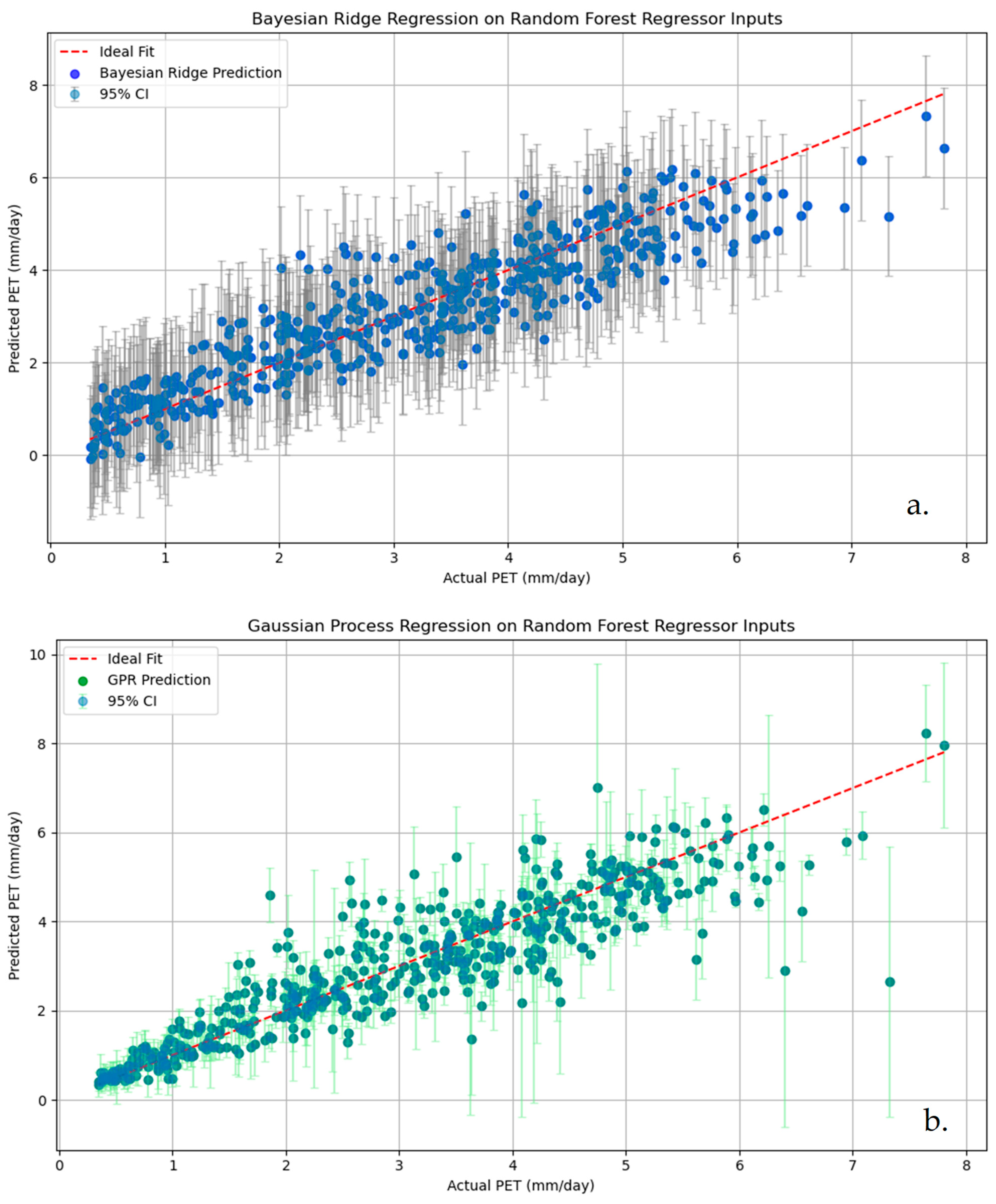
For Group 4 that produced the most accurate PET predictions, the Bayesian Ridge Regression and Gaussian Process Regression methods were employed to quantify uncertainty. Both methods provided 95% confidence intervals, allowing for a more robust assessment of prediction reliability. The results indicate that uncertainty increases for extreme PET values for both groups, aligning with prior research on ML biases (Figure 5).

The overall statistical assessment indicates that RFR is the most effective machine learning method to predict daily PET for the mountainous environment of a high-altitude Mediterranean study site. However, its optimal performance is achieved when using input parameters that include all temperature and relative humidity attributes (maximum, minimum, and average values) along with R_a. It is also important to underline that all machine learning models showed an adequate performance in predicting PET, yielding better statistical indices compared to relevant studies based on empirical models [9,53,54]. This is particularly important given the low data requirements, as it enables the production of relatively accurate daily PET estimates in regions or time periods with limited data availability. This is especially relevant considering that, in the past, standard meteorological stations typically measured only a few parameters, often excluding radiation attributes.

4. Discussion

Meteorological data (temperature, humidity, precipitation, etc.) are of the utmost importance for environmental sciences [55], since they are extremely useful, providing a scientific basis for the formulation of environmental protection policies and measures [56,57], crop and livestock production [58,59,60], ecological protection [61,62], responding to emergencies [63], and raising public awareness [64]. The datasets are usually obtained from meteorological networks installed and maintained by national agencies like National Oceanic and Atmospheric Administration (NOAA), Hellenic National Meteorological Service (HNMS), etc. While urban and peri-urban areas are well-covered by measurement station networks, rural regions often lack a similar infrastructure. The main reason for this is the increased cost for installing within a rural network, due to the sensor costs and maintenance [55].

This paper focuses on developing various ML regression algorithms for PET estimation in a high-altitude Mediterranean forest with limited meteorological data. Results indicate that ML algorithms, and especially RF, can provide high-accuracy PET estimates using only commonly available inputs, such as temperature, relative humidity, and extraterrestrial solar radiation estimated by geographical latitude. Recently, some works have reported the high performance of RF for the estimation of PET values under different climatic conditions [65,66,67]. Moreover, findings from this paper also validate a previous study in Greek lowland areas reporting that RF outperforms the rest of the ML regressors in the modeling of PET with temperature sensor data [37]. Additionally, the comparative analysis of several temperature-based empirical PET models against FAO-56 PM, applied in different sites in Greece [9,53,54], showed also weaker statistics compared to those of this study, suggesting that ML algorithms can be an excellent alternative for the estimation of PET.

Although predictive accuracy of the ML models was emphasized in the current study, their interpretability is equally crucial for application over data-poor mountain terrain where the transparent and explainable nature of decision-making becomes a priority. The Random Forest and Gradient Boosting algorithms naturally provide variable importance scores, which can identify the most significant meteorological drivers of PET (e.g., mean temperature, extraterrestrial radiation, or indices of humidity). Permutation importance and SHAP (SHapley Additive ex-Planations) analyses in a subsequent study will be used to graph the contribution of each feature, something which can influence priorities for installing the sensors and interpretating model output. The incorporation of such interpretability features will advance the operational utility of the models to the next level, making them actionable and interpretable to water planners and environmental managers

Notably, models using only the inputs from Group 2, temperature and extraterrestrial radiation, demonstrated strong predictability of PET, which reinforces the idea presented by Bellido-Jiménez et al. [35] that it is possible to estimate PET using minimal meteorological parameters. The addition of relative humidity in Groups 3 and 4 increased the accuracy indicating its important role as a supportive predictor. This can be partly attributed to the fact that relative humidity incorporates temperature as an attribute for its estimation and to the fact that the mountainous environment of our study site is generally characterized by high relative humidity values throughout the year and regardless of the season.

It is worth mentioning that regardless of the employed model, the inclusion of extraterrestrial radiation in the estimation of PET significantly enhances the performance of all models. This is to be expected considering that solar radiation is the main factor driving PET and thus, its intensity determines the water vapor fluxes. For this reason, the general pattern of Rs is followed by PET as depicted in Figure 4.

A recurring observation across all ML models was the systematic tendency to overestimate PET at lower values and underestimate it at higher values [68]. While this bias has been demonstrated to give accurate average predictions at an annual scale, it calls for tailored approaches to deal with extreme PET values. Among a range of methods to correct this bias, empirical distribution matching (EDM), ensemble approaches, and hybrid machine learning-empirical models have shown promising potential [69].

The usage of EDM requires that the model estimates the cumulative distribution function (CDF) of observed PET and predicted PET. Afterwards, the model matches the predicted PET values to their corresponding quantiles in the observed CDF.

The ensemble approaches which are essentially a combination of multiple models could also be used to deal with extreme PET values. In this case, we used a variety of trained models and then created a meta-model to combine their outputs and thus, reduce bias.

Finally, the combination of empirical PET models (like the FAO-56 Penman–Monteith) with predictions produced from machine learning models could also be used. In this case, we used both the empirical model and the ML model to estimate values and afterwards, we adjusted the ML predictions based on the empirical model estimates.

However, the reliability of ML diagnostic accuracy studies is often compromised by underreporting crucial experimental details and design features that may inflate accuracy estimates [70]. Publication bias also inflates the reported accuracy in ML-based studies; there is an inverse association between the sample size and reported accuracy [71].This credit also demonstrates the practical application of ML models in remote or data-scarce regions. It reduces dependence on expensive meteorological equipment by using widely available parameters of temperature and relative humidity and extraterrestrial radiation estimated from geographic coordinates. This fact becomes very important for a high-altitude atmospheric environment where installing, maintaining, and monitoring a conventional meteorological station is not inexpensive.

Compared to the FAO56 Penman–Monteith model, the gold standard for the estimation of PET, ML models are low-cost alternatives offering strong performances in specific contexts. Whereas the FAO56-PM requires many meteorological data, the ML approach, as noted in this study, has potential concerning site-specific applications and historical data reconstruction in areas characterized by data scarcity.

While this study focuses on a single high-altitude site in the Mediterranean region, its findings provide a valuable foundation for PET modeling in similar environments. Expanding this study to include additional sites across diverse climatic and topographic conditions would further enhance the generalization of the results. Coupling remote-sensing data, as indicated by Sharma et al. [24], may lead to overcoming some uncertainties related to local microclimates and increase the resolution of estimates in space. Among available remote sensing datasets, GLEAM (Global Land Evaporation Amsterdam Model) is a promising choice, as it provides satellite-based estimates of actual evapotranspiration using land surface temperature, radiation, and soil moisture as inputs. GLEAM outputs can be useful for PET validation and improving model calibration in data-scarce environments [72]. To further refine PET estimation in mountainous regions, higher-resolution remote sensing products should be considered. Landsat Thermal Infrared Sensor (TIRS) provides land surface temperature at a 100 m resolution, offering better spatial detail for PET modeling [73]. Sentinel-3 Sea and Land Surface Temperature Radiometer (SLSTR) deliver daily high-resolution land surface temperature data, which can improve PET estimation at regional scales [74]. Additionally, ECOSTRESS (ECOsystem Spaceborne Thermal Radiometer Experiment on Space Station) provides diurnal temperature variations at 70 m resolution, making it a valuable resource for capturing microclimatic fluctuations in complex terrain [75,76]. Future research should explore the integration of these datasets into PET estimation frameworks to assess their potential for improving spatial accuracy in mountainous environments.

Subsequently, the present study has highlighted the possibility of ML models and RF, particularly for the accurate, cost-effective estimation of PET over data-scarce, high-altitude regions. The results will contribute to sustainable water resource management and climate resilience strategies. Further work is required to be carried out by multi-site evaluations, remote sensing integrations, and the development of hybrid modeling frameworks for further advancements in the prediction of PET.

5. Conclusions

The accurate estimation of potential evapotranspiration (PET) is critically important in terrestrial ecosystem environmental modeling. The present work emphasizes the significant capability of machine learning (ML) methods in estimating PET under the adverse meteorological conditions prevailing in a mountainous Mediterranean forest site. Applying commonly available meteorological data, such as temperature, relative humidity, and the estimated extraterrestrial radiation, this study demonstrates a practical, low-cost alternative to conventional and computationally intensive methods like the FAO56 Penman–Monteith model.

The four ML algorithms evaluated in this study—Support Vector Regressor, SVR; Random Forest Regressor, RFR; and K-Nearest Neighbors, KNN—all demonstrated strong predictive performance for PET estimation. RFR consistently performed best across all different groups of input parameters whereas SVR outperformed the other ML model when using only temperature attributes. Including additional meteorological parameters generally improves model performance. This is evident in the results, as Group 1, which included only temperature attributes (T_mean, T_min, T_max), exhibited the lowest accuracy. Temperature alone does not fully capture the complexity of PET, as factors such as humidity and radiation proxy (R_a) significantly influence PET. When relative humidity (RH_mean, RH_min, RH_max) was introduced in Group 3, the PET estimates improved, indicating that humidity affects the accuracy of PET. However, even in the absence of humidity variables, Group 2—which incorporated extraterrestrial radiation (R_a) alongside temperature—outperformed Group 1. This highlights the strong influence of R_a on PET, as it directly governs available energy for evapotranspiration. The best performance was observed in Group 4, which combined both R_a and humidity parameters, reinforcing the importance of including comprehensive meteorological inputs in PET estimation models. These findings confirm that R_a, which can be readily computed based on geographical latitude, plays a crucial role in improving PET estimation accuracy, particularly when combined with other meteorological variables. One of the most important findings in this work is how ML models can work effectively in regions with minimal data availability. This flexibility is crucial for areas where conventional methods fall short due to resource or equipment limitations. Even excluding input parameters like relative humidity, the ML models still delivered accurate PET estimates, indicating the adaptability of these techniques to varying levels of data availability.

The research also points out areas for improvement. For example, all the tested models tended to overestimate low PET values and slightly underestimate higher ones, imposing a need for the development of more advanced techniques such as hybrid models or bias-correction methods. Additionally, a sensitivity analysis may be useful especially for evaluating the inclusion of extraterrestrial solar radiation as a proxy in the PET estimation models, which appeared to enhance the accuracy of estimated PET here but might not perform similarly in locations with more complex terrains in different microclimates. Finally, the hyperparameter tuning strategy could explore other optimization methods (genetic algorithms, grid search, Neural Architecture Search) to further optimize PET estimation accuracy and efficiency.

The findings of this research set a roadmap for broader applications of ML in hydrology and ecological modeling. Testing these models in other regions with different climates and terrains would help confirm their reliability. Larger datasets and technologies like remote sensing could also improve how well they capture local environmental nuances. Integrating ML models into hydrological and environmental assessment tools for water resource management and planning for climate change adaptation (such as vegetation water demand, crop water requirements, irrigation scheduling, hydrometeorological and climate classifications, drought identification and monitoring, etc.) can enhance their performance and make them even more impactful.

While this study focused on a specific Mediterranean mountainous forest site, we are aware that the extension of the developed models to other regions should be conducted cautiously. Differences in vegetation type, microclimate, elevation, and topographic complexity can all significantly impact PET dynamics. In order to assess the flexibility of the proposed approach, we plan to apply and test the same modeling scheme at a lower elevation site with an evergreen oak forest, where similar meteorological equipment has been set up. This activity will allow us to examine how model performance changes with various physiographic and climatic conditions and to test the method’s robustness and scalability under varying Mediterranean environments.

In conclusion, ML models—especially RFR—show great promise for estimating PET in data-scarce regions. They offer a practical, low-cost way to fill gaps in environmental data and support better resource management. As water scarcity and climate challenges grow, solutions like these will become increasingly valuable.