Article

Climate Projections and Time Series Analysis over Roma Fiumicino Airport Using COSMO-CLM: Insights from Advanced Statistical Methods

by
Edoardo Bucchignani
Centro Italiano Ricerche Aerospaziali (CIRA), Via Maiorise, 81043 Capua, CE, Italy
Atmosphere 2025, 16(7), 843; https://doi.org/10.3390/atmos16070843
Submission received: 28 May 2025 / Revised: 5 July 2025 / Accepted: 10 July 2025 / Published: 11 July 2025
(This article belongs to the Section Climatology)

Abstract

The evaluation of climate change effects on airport infrastructures is important to maintain safety and flexibility in air travel operations. Airports are particularly vulnerable to extreme weather events and temperature fluctuations, which can disrupt operations, compromise passenger safety, and cause economic losses. Issues such as flooded runways and the disruption of power supplies highlight the need for strong adaptation strategies. The study focuses on the application of the high-resolution regional model COSMO-CLM to assess climate change impacts on Roma Fiumicino airport (Italy) under the IPCC RCP8.5 scenario. The complex topography of Italy requires fine-scale simulation to catch localized climate dynamics. By employing advanced statistical methods, such as fractal analysis, this research aims to increase an understanding of climate change and improve the model prediction capability. The findings provide valuable insights for designing resilient airport infrastructures and updating operational protocols in view of evolving climate risks. A consistent increase in daily temperatures is projected, along with a modest positive trend in annual precipitation. The use of advanced statistical methods revealed insights into the fractal dimensions and frequency components of climate variables, showing an increasing complexity and variability of future climatic patterns.

1. Introduction

The evaluation of the effects of climate change on airports is important to ensure the flexibility and safety of the infrastructure of air travel. Airports are unsafe in temperature oscillations and extreme weather events, which can disrupt operations and compromise passenger safety. For example, the flooding of runways and terminal areas may cause expensive damage and flight delays. High temperatures can affect the performance of the aircraft, requiring a long runway for safe takeoff. Additionally, the disruption of ground transport and power supplies caused by extreme weather can obstruct the functionality of the airport. Understanding these risks enables better planning and adaptation strategies, such as re-designing the infrastructure, increasing drainage systems, and updating the operational protocol. The methodologies for quantifying the potential effects of climate change on the aviation sector are still limited, especially in the Mediterranean area [1], although this region has been defined as a climate hot spot [2]. As explained in [3], the first step required to define a framework for risk assessment is the identification of relevant climate change projections over the 21st century and their potential impacts on airport infrastructures. Global climate models (GCMs) are powerful tools for the analysis of large-scale climate processes, but they lack the high resolution required to capture fine-scale features for regional decision-making. Regional climate models (RCMs) are able to remove this gap by providing details into localized climate dynamics, such as temperature variations, precipitation, and extreme weather events. These simulations support a deep understanding about the climate trends in specific areas, considering factors like topography, land use, and local climate conditions. This localized information is essential for sectors such as agriculture, urban planning, and disaster management, to drive informed strategies for mitigation and adaptation to climate change impacts. In the last decade, several initiatives, e.g., the WCRP Coordinated Regional Downscaling Experiment (CORDEX) project [4], were established to provide a global coordination of RCM downscaling for climate change adaptation and impact assessment. In the field of aviation, these localized insights are critical for the assessment of risks such as turbulence, storm frequency, and changes in jet stream dynamics, all of which directly affect flight safety, fuel efficiency, and scheduling reliability. High-resolution RCMs also allow a better representation of extreme weather events (i.e., thunderstorms and icing conditions) that could represent significant operational challenges. By incorporating this information into an aviation risk management framework, stakeholders and policy makers can develop more resilient strategies to mitigate climate-related disruptions, ensuring more efficient air travel even in a changing climate. Furthermore, due to the complex nature of climate phenomena, some studies [5] suggest performing specific analyses of climate time series by using advanced statistical methods because of the lack of regularity of occurrences. An exhaustive review of the application of a fractal analysis on wind speed time series is presented in [6]. The analysis of climate time series with tools like FFT or the Higuchi method [7] is critical for understanding the intrinsic complexity and dynamics of climate systems. These methods allow us to quantify patterns and structures, revealing properties like persistence or fractality. For instance, the dimension obtained through Higuchi’s approach can distinguish between chaotic, random, or persistent trends, providing information on the underlying processes driving climate variability. This is essential for improving predictive models and assessing long-term trends, such as those related to climate change. The visualization and quantification of these dynamics can support policy decisions aimed at mitigating climate risks.
Over Italy, detailed analyses of the impacts of climate change in the aviation sector are still limited. In [8], the expected climate extreme variability over Capodichino airport, located in Naples (Italy), was analyzed. De Vivo et al. [9] applied a climate risk assessment framework to evaluate the impacts of extreme temperatures on several Italian airports. ALBATROS (Advanced systems and solutions for better practices against hazards in the aviation system) is a Horizon Europe-funded project whose ambition is to maintain a high level of safety and resilience in aviation in view of extreme weather conditions. In this frame, the Italian Aerospace Research Center (CIRA) has conducted high-resolution climate simulations using the RCM COSMO-CLM over a geographical area centered over Roma Fiumicino Airport (Italy), in order to provide climate projections according to IPCC RCP8.5 scenario, which is often adopted as a benchmark for understanding the potential impacts of unmitigated climate change. The Italian peninsula is a geographical area that requires high-resolution climatology (less than 10 km) due to its highly complex topography, which encompasses high mountain ranges and a diverse array of coastlines.
The main aim of this work was to provide climate projections over Roma Fiumicino airport, widening the range of projections already available in the literature for this area, but with a higher resolution, employing the “state-of-art” latest version of COSMO-CLM. The novelty of this paper lies in the fact that, for the first time, advanced statistical techniques have been applied to climate projections performed for an Italian site. This approach provides valuable insights into the expected climate dynamics in the coming years. By combining high-resolution RCM outputs with sophisticated post-processing methods, the study offers a reliable perspective on future climatic trends, contributing to a deeper understanding of climate behavior and its potential impacts.
This paper is organized as follows: Section 2 contains a description of the methodology employed, including RCM and simulations set-up; Section 3 reports the comparison of the model results with respect to the observations, whereas climate projections are analyzed in Section 4. Conclusions and discussion are reported in Section 5.

2. The Methodology Employed

2.1. The RCM and Simulation Set-Up

The three-dimensional, non-hydrostatic regional model COSMO-CLM [10] is the climate-adapted version of the operational weather forecasting model COSMO-LM [11], originally developed by the German Weather Service (DWD). It is based on the Navier–Stokes equations for a compressible flow and assuming a hydrostatic base state at rest. The atmosphere is modeled as a multicomponent fluid consisting of dry air, water vapor, and liquid and solid water, all of which obey the ideal gas law. This fluid is influenced by gravitational and Coriolis forces. Small-scale phenomena that cannot be explicitly resolved are incorporated using statistical approaches implemented through various parameterization schemes. The COSMO-CLM version used in this work is 6.0_clm2. The development of the COSMO model ended in 2021; in fact, COSMO 6.0 was released on 15 December 2021 and it was the last release of the COSMO model. In this version, several diagnostic output variables were added, for example for wind sector classes and for sunshine duration. Also, new tuning variables have been introduced for several parameterization schemes. A new additional hydrology scheme (groundwater and runoff) has been developed.
In this study, a preliminary experiment was carried out by using ERA5 as forcing [12], which is a high-resolution global reanalysis dataset by the European Centre for Medium-Range Weather Forecasts (ECMWF). It is characterized by a spatial resolution of 0.25° (about 31 km) and a temporal coverage from 1940 to the present. The quality of this dataset makes it ideal for providing perfect initial and boundary conditions to RCMs, enabling the study of localized climate phenomena with great accuracy. The simulation covers the period 1979–2010 and uses the computational domain (2–22° E; 35–49° N) shown in Figure 1. The grid is characterized by a spatial resolution of 0.0715° (about 8 km) and has 185 × 195 grid points. The time integration is based on a third-order Runge–Kutta scheme, convection is parameterized using the Tiedtke scheme [13], while the number of vertical levels in the atmosphere and the number of soil levels are set at 40 and 9, respectively. The sponge zone is made up of 15 grid points.
The main experiment was driven by the GCM EC-Earth at 1.125° (about 128 km) resolution. The GCM EC-Earth (Earth System Model) [14] is a state-of-the-art global climate model developed by a consortium of European institutions. It simulates the global climate system, integrating atmospheric, oceanic, land surface, and sea ice processes. It was built upon the ECMWF Integrated Forecasting System (IFS) and was designed for weather prediction and climate research. Specifically, it is used for the study of past periods and future climate scenarios, contributing to several projects (i.e., IPCC assessments) and advancing the understanding of climate dynamics and variability. This experiment used a double nesting approach: the first simulation was performed over the period 1979–2050 using a coarser grid (resolution 0.44°, about 50 km) on the domain (30° W–54° E; 22–66° N) that includes 95 × 95 grid points; the number of vertical and soil levels are set at 40 and 9, respectively. The second simulation was performed using the same computational grid already adopted in the preliminary experiment (resolution 0.0715°), with initial and boundary conditions provided by the previous 0.44° simulation, over the period 1980–2050 (the year 1979 was removed to reduce the spin-up period influenced by initial conditions).

2.2. The Case Study Area and Observational Datasets

In the frame of the ALBATROS project, a group of representative European airports was selected to investigate the potential impacts of climate change, covering the main climate regions as defined by the European Environment Agency map. To ensure a comprehensive analysis, two airports were chosen from each region, i.e., a large airport and a smaller one. In particular, Roma Fiumicino was selected as large airport of the Intermediate Subtropical climate region and CIRA was in charge of the related investigation. As discussed in [15], Fiumicino airport is exposed to an increased risk of extreme weather events, such as heatwaves, heavy rainfall, and flooding, which could interfere with airport operations, cause damage to infrastructure, and increase maintenance costs. In addition, climate change could affect safety, for example by increasing the risk of bird strikes due to changes in local ecosystems. Moreover, as shown in [16], Fiumicino is classified in the high and very high-risk class in all IPCC scenarios, especially for what concerns extreme temperatures.
A model evaluation for the entire Italian domain was conducted using the E-OBS (version 29) gridded dataset [17] at a resolution of 0.10°. E-OBS provides daily mean values for several variables, such as precipitation and temperature, over the period 1950–2023. It was developed by interpolating one of the most comprehensive collections of station data across Europe. The dataset advantage lies in its extensive spatial and temporal coverage, making it a standard reference for climate research and a widely used tool for evaluating RCMs across Europe. In this study, seasonal bias maps of mean, 2 m above ground air temperature and total precipitation, have been analyzed, obtained by comparing the values of simulation output with the E-OBS considering the time period 1981–2010. To this aim, the model data were interpolated onto the dataset grid using the bilinear interpolation. Furthermore, in order to obtain a more detailed performance evaluation over Roma Fiumicino airport, the annual cycle of the investigated variables were computed for all the simulations performed considering the nearest grid point to the airport location. In this case, in addition to the E-OBS dataset, the station data from the SCIA system (National System for the collection, elaboration, and diffusion of climate data) developed by ISPRA (Istituto Superiore Protezione e Ricerca Ambientale) [18] has also been used for the comparison.
The BIAS index (Model minus Observation) has been used for performance evaluation, which is defined as
B I A S = 1 N i = 1 N S i O i
in which Si and Oi are the simulated and observed monthly values averaged over the domain considered at the ith month and N is the number of months in the evaluation period.

2.3. Statistical Methods for the Analysis of the Results

The Fourier transform is a powerful tool for signal analysis, but it is subject to certain limitations. For example, a chaotic regime is characterized by a continuous power spectrum, however a Fourier spectrum that looks continuous cannot be automatically attributed to a chaotic signal, since it can be also representative of a quasi-periodic signal with a high number of frequencies (white noise) [19]. For this reason, a Fourier analysis (e.g., FFT) could not be sufficient to characterize a chaotic signal. The measurement of the fractal dimension of an attractor provides important information about the kind of temporal regime that characterizes a dissipative system [20], since the fractal dimension measures the number of relevant degrees of freedom. The Higuchi method [7] is a powerful tool that can be used to capture the intrinsic complexity of time signals. It is based on the construction of several time sub-series, starting from the original one (N elements). For a given parameter k, the algorithm splits the time series into sub-series whose distance is k, evaluates the length L of them, and calculates the average value:
L k m = 1 k i = 1 N m k x m + i · k x m + i 1 · k · N 1 N m k · k
L k = 1 k m = 1 k L k ( m )
with m = 1, 2, … k. The process is repeated for several values of k and then the fractal dimension d is evaluated as the slope of the log–log relationship between the average length of the curve and k. Values of d close to 1 are representative of a relatively simple and regular time series, while values of d close to 2 are related to complex and non-regular signals. For atmospheric variables, a fractal dimension close to 1 indicates a strong positive persistency, which is representative of a regular time series that reflects foreseeable and stable climate cycles (e.g., annual seasonality). An intermediate value of d (about 1.3) indicates a limited persistency or a non-linear dynamic, in other words the series features a deterministic and a random component. Finally, higher values imply that the series shows non-regular fluctuations, associated with climate changes or extreme weather phenomena. The analysis of changes in the value of d over future periods with respect to past ones could help to record whether the system is becoming more complex or less foreseeable.

3. Model Evaluation

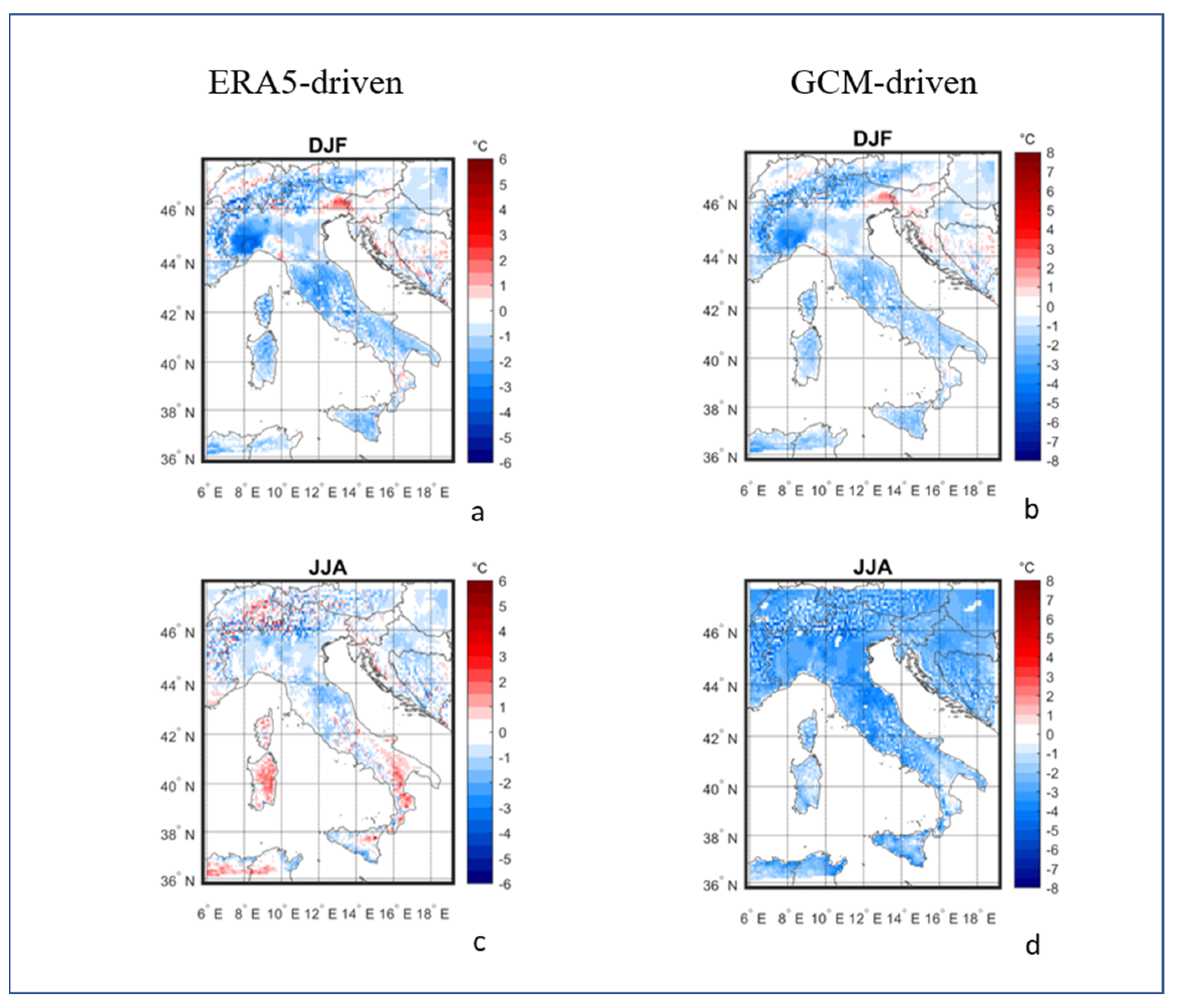
This section is devoted to the quality assessment of climate model data. The mean 2 m temperature (T_2m) seasonal bias distributions over the period 1981–2010 are shown in Figure 2, for winter (DJF) and summer (JJA), respectively, for ERA5- (a–c) and GCM EC-EARTH- (b–d) driven simulations. The color scale indicates temperature bias in °C, with blue showing areas where the model underestimates temperature and red for overestimations. For ERA5-driven, a pronounced underestimation is recorded in winter over the Alps, potentially due to difficulties in simulating complex topography or snow-albedo feedbacks. Smaller biases are observed in southern Italy and islands. In summer, a slight temperature overestimation is visible in southern Italy and Sardinia, which might reflect challenges in simulating heatwaves [21], soil moisture dynamics, and urban heat effects [22]. An underestimation persists on northern and central Italy. For GCM EC-EARTH-driven, panels b-d suggest that COSMO-CLM generally is affected by a cold bias across Italy, with intensity depending on the season. In winter, the cold bias is particularly pronounced in northern Italy whereas minor overestimations (red areas) are visible in limited regions, such as north-eastern Italy. The cold bias is stronger during JJA, suggesting that the model has difficulties simulating warmer temperatures; coastal regions and islands show smaller biases compared to inland and mountainous areas. This general cold bias is inherited by the driving GCM, in fact the temperature underestimation by the EC-Earth model over Italy (and other specific regions) has been reported in some analyses and scientific publications. As regards bias in summer temperatures, recent studies (e.g., [23]) have indicated that EC-Earth tends to underestimate temperatures in Italy and other areas of the Mediterranean, and that this could be due to an incomplete representation of the feedback between dry soil and high temperatures. Regarding the topographic influence, the complex orography of Italy may be too simplified in the model, leading to an underestimation of temperatures in certain areas (e.g., plains or coastal regions). The latest version of EC-Earth has improved spatial resolution and the representation of certain key processes, reducing some biases. However, the extent of these improvements may vary depending on the model configuration (e.g., atmosphere–ocean coupling, and the resolution used). A recent study [24] analyzed the very high-resolution configuration of the EC-Earth model for “The High-Resolution Model Intercomparison Project (HighResMIP)”, comparing it with lower-resolution versions. The results indicate that, despite improvements in the representation of certain climatic phenomena, biases persist in the simulations of summer temperatures in Europe, highlighting the need for further refinements in the model. Table 1 reports the values of the BIAS index for the performance evaluation of T_2m, averaged over the whole domain considered, for both simulations and seasons. These values confirm the good performances of the ERA5-driven simulation, even if some compensation effects may exist.
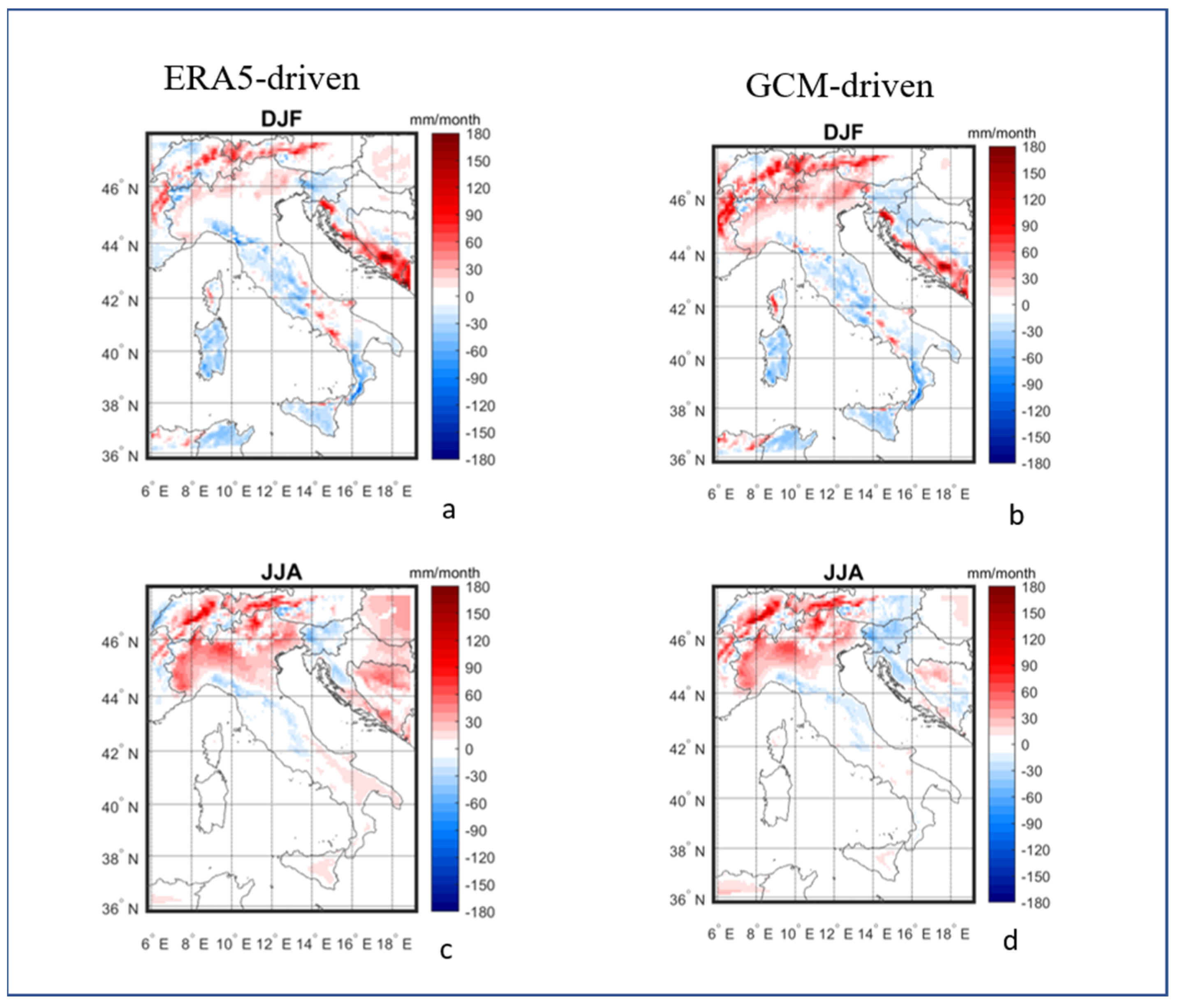
Figure 3 shows the seasonal precipitation bias (mm/month) of the ERA5-driven simulation (a–c) compared to the E-OBS dataset for the period 1981–2010, with blue indicating an underestimation and red indicating an overestimation. In winter, a positive bias is recorded in the northern part of the domain, whereas negative biases affect the Apennines and southern Italy. In summer, precipitation is slightly overestimated in the north, which might be related to excessive convective activity simulated by the model. For GCM-driven simulations (b–d), results highlight strong spatial and seasonal variations, with notable differences in northern Italy compared to central and southern regions. In DJF, an overestimation is observed in the northern regions, particularly along the Alps whereas some underestimations occur in southern and central Italy. In JJA, northern Italy shows an overestimation, although the magnitude is reduced compared to winter. Underestimations are more widespread across central Italy, likely due to the model underestimating convective precipitation during the summer. BIAS values related to precipitation are also shown in Table 1, which confirm the good performances in winter and a relevant overestimation in summer, for both simulations.
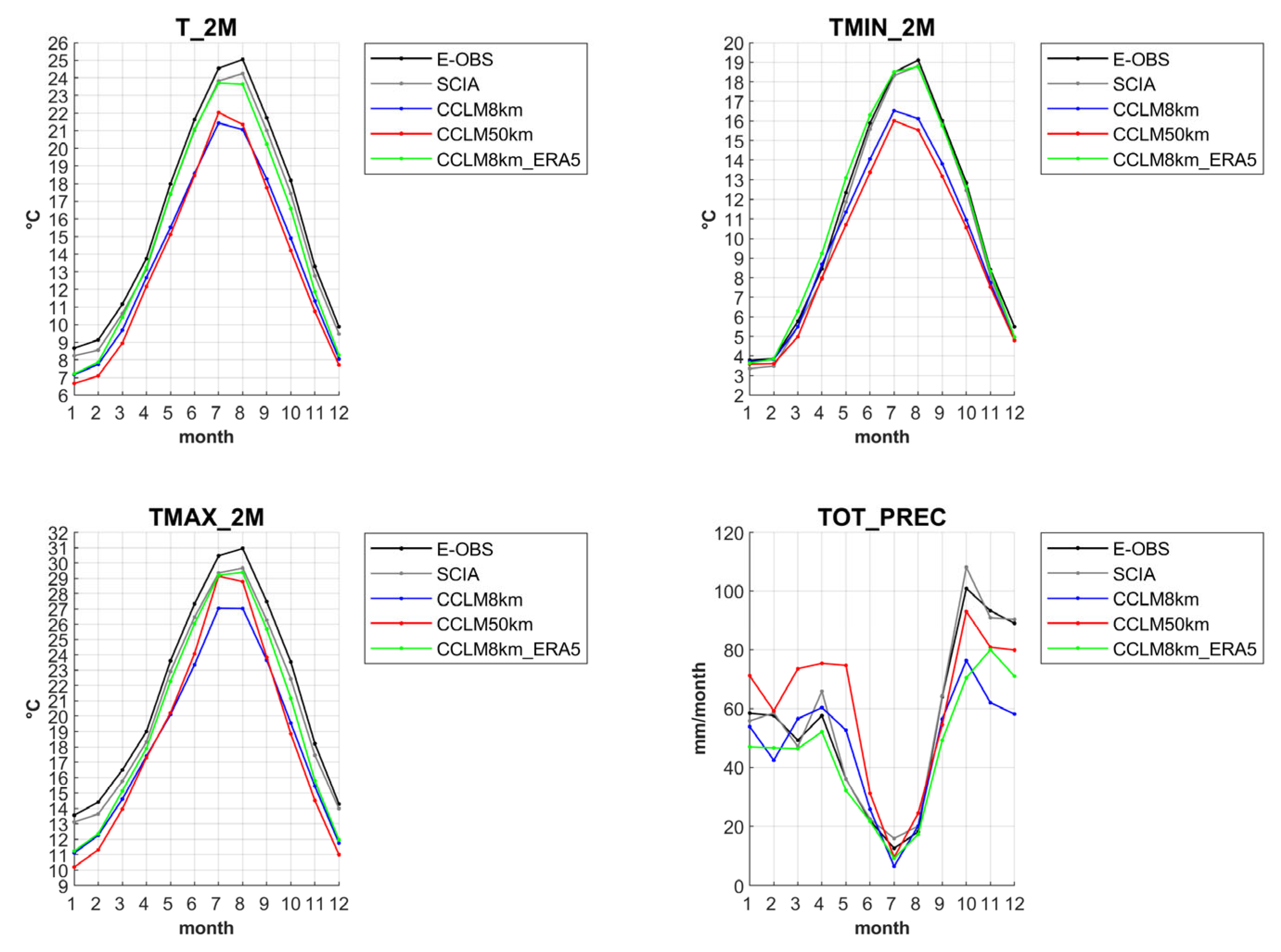
The annual cycles of 2 m daily mean (T_2m), maximum (Tmax_2m), minimum temperature (Tmin_2m) and total precipitation (Tot_Prec) for the Roma Fiumicino airport location are shown in Figure 4. Data are provided by ERA5- and EC-Earth-driven simulations at both the resolutions considered (0.44° and 0.0715°), averaged over the period 1981–2010, obtained considering the nearest grid point to the location considered. They have been compared to annual cycles provided by the E-OBS dataset (nearest grid point) and ground station data from the SCIA system. The ERA5-driven simulation is characterized by great accuracy, while EC-Earth-driven exhibits a systematic cold bias for mean, maximum, and minimum temperatures, with the bias increasing during warmer months. Generally, the coarse resolution underperforms compared to the finer one, with the exception of the maximum temperature in summer. Regarding precipitation, during spring the EC-Earth-driven simulations are characterized by a general overestimation, more pronounced for the coarser one, whereas the ERA5-driven simulation shows a slight underestimation. From September to December, instead, all the simulations underestimate the observed values, especially the run at 0.0715° forced by EC-Earth. The annual cycles have been computed also considering the average value over a 3 × 3 grid box centered on the nearest point to the airport location. The results are generally similar to the ones obtained considering the single closest point, with the exception of the simulation at a 0.44° resolution, since the analyzed area is much larger due to the greater distance between the points included in the box.

4. Analysis of Climate Projections

Climate projections have been performed under the IPCC RCP8.5 (Representative Concentration Pathway 8.5) scenario [25]. It is a high greenhouse gas concentration scenario, often referred to as a “business-as-usual”, which assumes a continued growth in fossil fuel use and limited mitigation efforts, resulting in a radiative forcing of 8.5 W/m2 by 2100. This scenario projects a significant increases in global temperatures, rising sea levels, and increasing extreme weather events, serving as a benchmark for understanding the potential impacts of unmitigated climate change. The significance of the projections was assessed by applying the Mann–Kendall nonparametric test, assuming a confidence level of 95%.
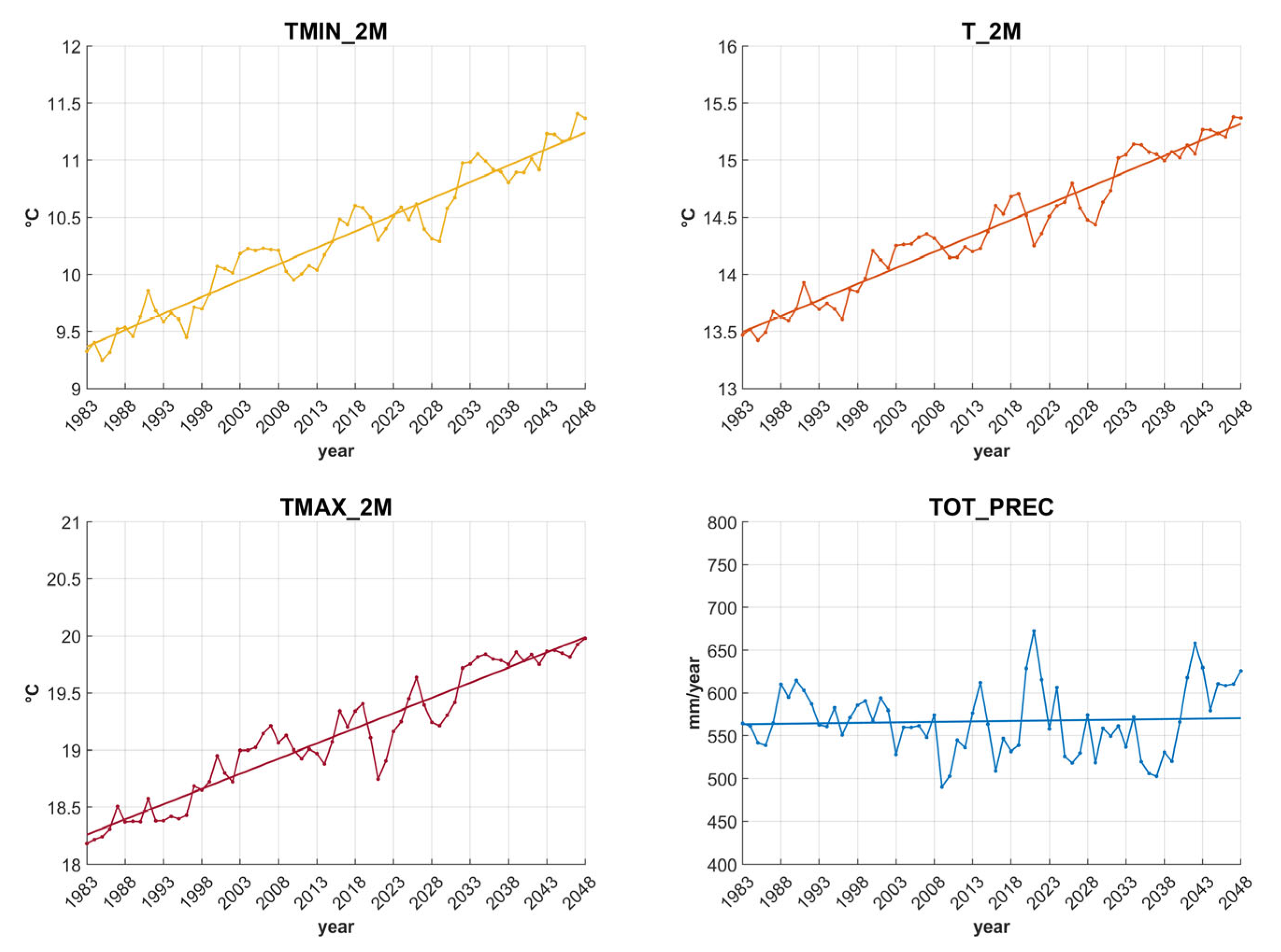
Figure 5 shows the yearly time series (5-year running mean) covering the period 1981–2050 of daily (mean, maximum, and minimum) 2 m temperature and total precipitation at Rome Fiumicino (nearest grid point). For temperature, a positive trend is projected (0.028, 0.027 and 0.029 °C/year for mean, maximum, and minimum, respectively), which could exacerbate heatwaves, drought conditions, and energy demands for cooling, as well as pose health risks. These implications derive from the projected warming in combination with the existing literature and historical patterns. For precipitation, a modest positive trend is also detected (0.109 mm/year), with annual precipitation fluctuating between 490 mm and 673 mm; this large variability could result in more intense rainfall events, with possible implications for flooding, droughts, and water resource management.

4.1. Analysis of Daily Time Series and FFT

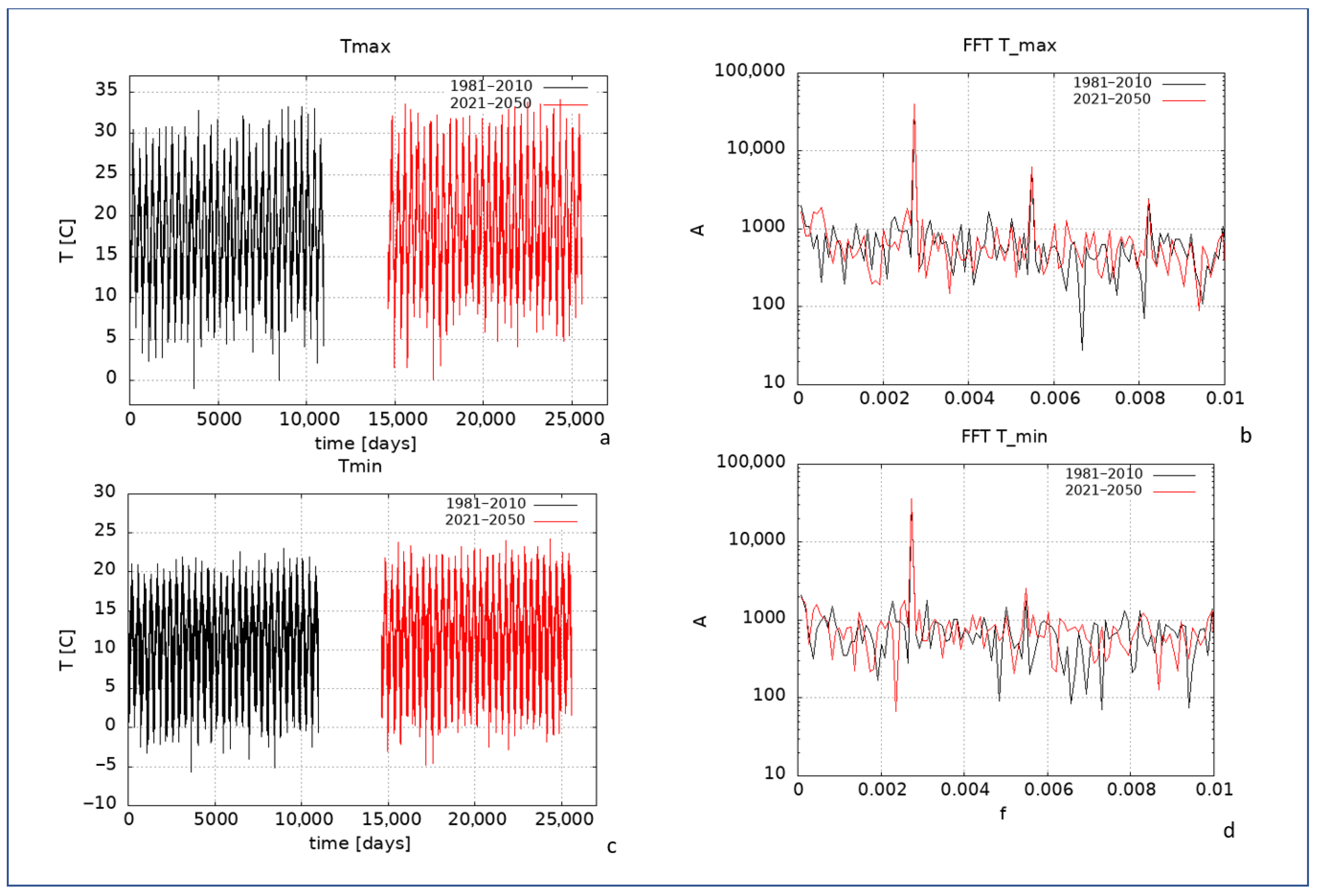
A daily time series of 2 m maximum and minimum temperature, total precipitation, and 10 m wind speed, covering the periods 1981–2010 and 2021–2050, were processed using an FFT to produce a power spectrum of the corresponding variables at regularly spaced bins, in order to measure the amounts of variability occurring in different frequency bands. The frequency resolution is 1/T0 = 0.912 × 10⁻⁴ (given that T0 is 10,957 d). The values of the main periods recorded (in days) for the variables considered are shown in Table 2. Figure 6a–c shows the time series of daily 2 m maximum and minimum temperature over the periods considered, while Figure 6b–d shows the corresponding mean power spectra. For Tmax_2m, a regular pattern in the time series can be observed, while three main peaks are visible in the power spectrum (f = 2.74 × 10⁻³, 5.48 × 10⁻³, 8.21 × 10⁻³), corresponding to periods of 365, 182, and 121 d, respectively. The first one corresponds to the annual cycle of temperature, dominated by seasonal variations. The second one refers to variations that are repeated every 6 months, reflecting temperature changes related to seasonal transitions (e.g., winter–spring and summer–autumn). Moreover, higher harmonic frequencies may arise if heating and cooling are not uniform over the year. Both past and future periods show a similar behavior at low frequencies, while at high frequencies (>0.005) a slight attenuation of the amplitude is observed in the future period. This could be related to a reduction in rapid (day-to-day) fluctuations, linked to a greater persistence of warm events or a more uniform climate on short time scales. For Tmin_2m, in both periods a similar trend is recorded for low frequencies (T = 365 d) with comparable amplitudes. At higher frequencies, amplitudes are slightly different for the two periods, suggesting a potential reduction of the fast variations in Tmin_2m in the future, with a more stable climate.
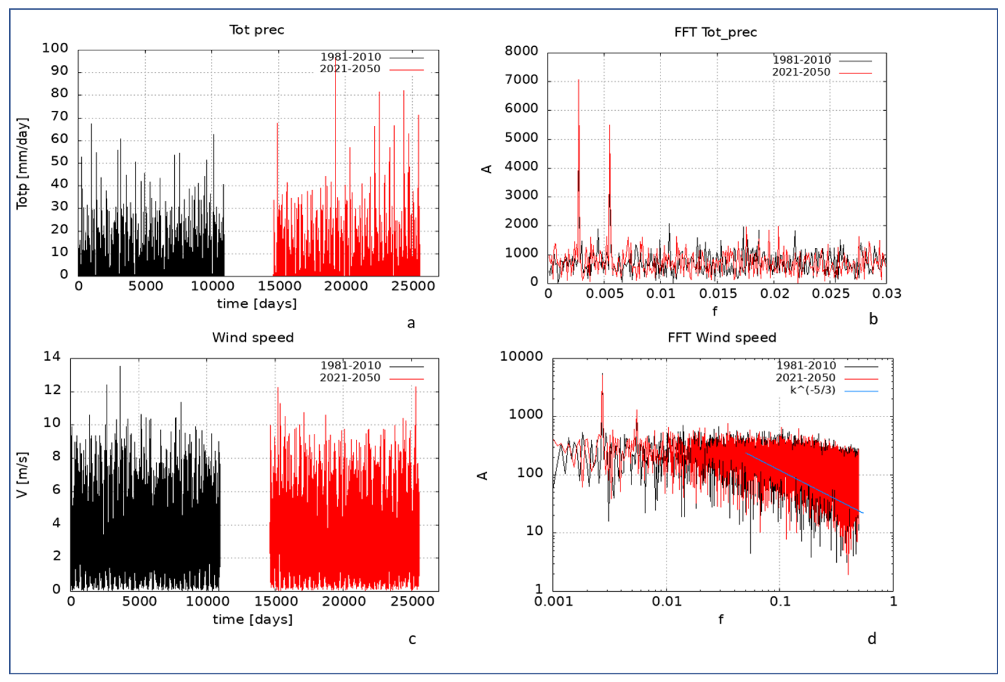
Figure 7a–c shows the time series of daily total precipitation and 10 m wind speed over the periods considered, while Figure 7b–d shows the corresponding mean power spectra. For precipitation, significant peaks in the amplitude spectrum are observed around low specific frequencies. These peaks indicate the presence of dominant periodic cycles in precipitation, probably related to seasonal or interannual climate phenomena. The main peaks are present in both past and future periods, suggesting that some periodic features persist over time. The future series generally presents a slightly larger amplitude than the historical series in some frequencies, especially around the main peaks, indicating an intensification of some cyclical components of precipitation in the future. The spectral noise appears slightly more pronounced in the future, reflecting greater climate variability in future precipitation. These results project a change in the intensity or periodicity of future precipitation events. In particular, an increase in spectral amplitude at certain frequencies may reflect more intense weather events, considering that any changes in the identified cycles could be associated with global climate processes, such as changes in atmospheric circulation. For the 10 m wind speed, the same peaks in the amplitude spectrum are observed for both time series around low specific frequencies. Moreover, the spectra (log–log representation) at high frequencies generally show a declining trend with noise superimposed. At higher frequencies, the observed distribution has been compared with the power law described by Kolmogorov for homogeneous isotropic turbulence (depicted as a blue line in the figure). According to Kolmogorov’s theory [26], the velocity spectrum of turbulence can be divided into distinct frequency ranges, often classified as the turbulence source region (large scale), the inertial subrange (medium scale), and the dissipation region (small scale). This law [27] asserts that, assuming a constant energy dissipation rate, the energy of turbulent flow depends solely on the scale of turbulence raised to the −5/3 power. From the figure, it is clear that at higher frequencies, the wind power spectrum aligns closely with the Kolmogorov distribution. However, it is crucial to emphasize that the Fourier power spectrum is a second-order statistical measure, providing insights into medium-level fluctuations but not fully characterizing the scaling process.

4.2. Evaluation of Fractal Dimensions

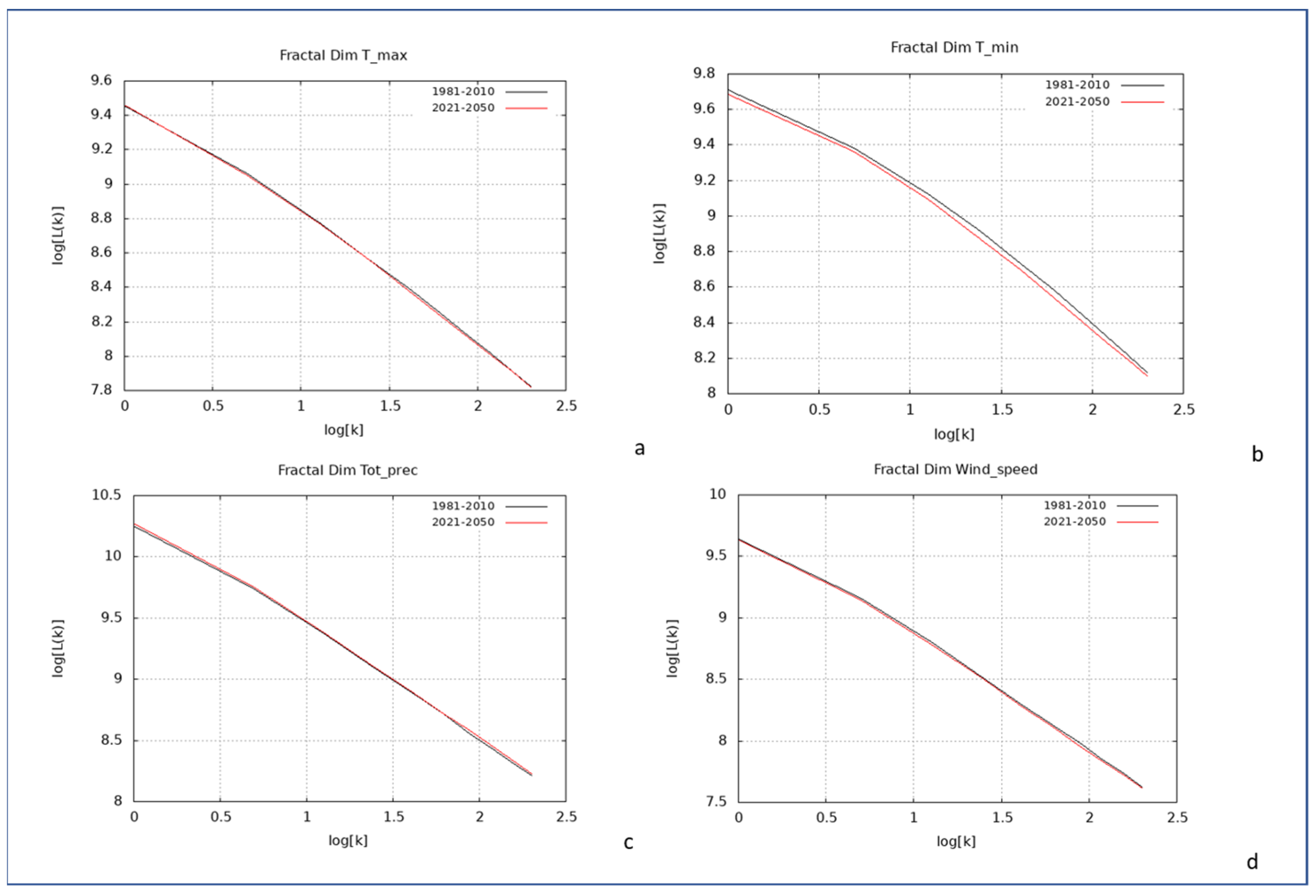
The values of fractal dimensions (d) represent a measure of the complexity and variability of the time series. Values of d associated with the daily time series already described were calculated by means of the Higuchi method, which allows the assessment of irregularity and seasonal patterns in the variables. These patterns are influenced by various atmospheric factors and environmental conditions (including topographical features) operating across multiple scales and temporal frequencies. Figure 8 shows the log–log plots of the relationship between L(k) and k for the four variables considered, for both past and future periods, which is the basis of the evaluation of the fractal dimension. Table 3 contains the corresponding values of the fractal dimensions. For Tmax_2m, the complexity will slightly increase in the future, which could be related to a growth of the daily thermal variability or to a larger number of extreme events. A larger increase is recorded for Tmin_2m, which could be associated with phenomena such as warmer nights or a larger nocturnal variability. For total precipitation, the value of d remains almost unchanged, implying that climate changes do not have a significant impact on the temporal variability of total precipitation. For the 10 m wind speed, the expected variation of d is small too, revealing that changes in the temporal structure of wind are limited, with a stable complexity over the time. Overall, the expected increases of d for temperature in the future are related to the effects of climate change, which introduce new patterns in the temporal distributions of extreme events, such as heat waves.
Several studies suggest that the fractal dimension of a wind speed time series is a measure not only of turbulent complexity, but also of the stability conditions of the atmospheric boundary layer (ABL). In particular, Tijera et al. [28] showed that the fractal dimension is influenced by the stability of the boundary layer, characterized by the Bulk Richardson Number (RiB), which compares buoyant and shear forces. In particular, they found that under instability conditions (RiB < 0) the fractal dimension remains constant (about 1.15). Under neutral conditions the fractal dimension is maximum and then it decreases rapidly for stable conditions (RiB > 0). Shu et al. [29] investigated the vertical wind speed variability in the context of fractal dimension analysis, showing that the time series of vertical wind velocity are monofractals and weak anti-persistent. Moreover, the median fractal dimension decreases from 1.582 at 10 m to 1.547 at 320 m, with a vertical profile linked to atmospheric stability, influencing both its values and shape, with the greatest deviations occurring at higher altitudes. Additionally, the fractal dimension tends to increase with rising horizontal wind speed, partly due to the influence of atmospheric stability. This relationship also varies with altitude. Xia et al. [30] investigated the fractal characteristics of wind speed during the transit periods of four typhoons, finding values between 1.3 and 1.5, indicating the complexity of wind speeds during typhoon landfall.

5. Conclusions and Discussion

In the present work, climate simulations performed with the RCM COSMO-CLM model over a geographical area centered over Roma Fiumicino airport have been performed and analyzed. The study emphasized the critical role of high-resolution regional climate modeling in understanding localized climate impacts. As regards the ERA5-driven simulation, a general slight underestimation of temperature is evident in all the seasons, stronger in winter. Negative precipitation biases in central Italy suggest difficulties in capturing Mediterranean storm dynamics and convective rainfall. As regards the EC-Earth-driven simulation, COSMO-CLM consistently underestimates temperatures in all seasons, which is mostly inherited by the global model, but could be also related to errors in simulating topography or snow cover. These biases reveal challenges in accurately capturing temperature dynamics, possibly due to parameterizations of surface energy fluxes, vegetation, or atmospheric processes. Overall, the present analysis highlights that in some areas model improvements are needed, particularly in handling winter cold extremes, summer heat events, and the representation of topographic influences, implying that bias correction techniques might be required when using RCMs for impact studies or decision-making processes.
For the specific area of Roma Fiumicino airport, the analysis under the RCP8.5 scenario projects a consistent increase in daily mean, maximum, and minimum temperatures, with trends of 0.028 °C/year, 0.027 °C/year, and 0.029 °C/year, respectively, which could exacerbate heatwaves, increase energy demands for cooling, and heighten health risks. Warmer nights could lead to reduced nocturnal cooling, affecting energy demands and increasing the heat stress on ecosystems and urban populations, while higher maximum temperatures could intensify heatwaves and increase risks for health, agriculture, and energy systems [31,32]. Similarly, a modest positive trend in annual precipitation (0.109 mm/year) is detected, highlighting increased variability and a potential rise in extreme rainfall events. The area may experience a combination of warmer conditions and precipitation variability, leading to urban planning challenges such as heat stress, flood control, and infrastructure resilience [33]. These changes underline the importance of developing adaptation strategies for aviation (e.g., runway reinforcement, heat-tolerant materials, and fuel efficiency innovations) and other sectors, such as agriculture, water management, urban planning, and public health.
These outcomes are consistent with previous studies [34], confirming the broader trends of climate change impacts over the Mediterranean regions. Moreover, the results provide novel contributions by offering high-resolution projections specific to the Fiumicino airport area, enabling a more detailed assessment of potential risks and adaptation needs. Furthermore, the use of advanced statistical methods, such as the Higuchi method and FFT analysis, revealed insights into the fractal dimensions and frequency components of climate variables, showing an increasing complexity and variability of future climatic patterns. Then, the methodological advancements demonstrated in this study provide a framework for assessing climate impacts in other regions with similar topographical and climatic features. Nevertheless, some limitations should be acknowledged, such as the inherent uncertainties associated with climate modeling and the reliance on a single model and a single IPCC scenario. In fact, according to the IPCC report [35], the projection reliability might be improved by using multi-model ensembles, weighting the elements according to the model skills. Ensembles are useful for the quantification of uncertainty, which is fundamental in the decision-making processes. This analysis will be the object of future works, in particular when CMIP6-driven simulations at high resolution will be available over Italy. Moreover, to overcome the mentioned limitations, other methodologies will need to be considered. For example, the integration of fractal analysis with AI techniques, such as artificial neural networks and neuro-fuzzy systems, has proven effective in improving wind speed prediction accuracy. A study by Petković et al. [36] highlighted the synergy between fractal extrapolation and AI methods in addressing the complexities of a wind speed time series. Fractal metrics, when integrated with machine learning, could enhance model performance by quantifying complexity and refining data decomposition [6]. These metrics aid in the tuning of hyperparameter and the trend identification, improving predictive accuracy and reducing the computational overhead. In applications like wind speed forecasting, fractal analysis efficiently allocates resources by identifying components that significantly impact forecasting errors. Furthermore, the integration of physics-informed models, combining domain expertise with fractal techniques and machine learning, could offer a more accurate approach to climate change projections. This study was performed in the frame of the Horizon Europe ALBATROS project, which focuses on ensuring safety and resilience in aviation under extreme weather conditions. The results support informed decision-making for climate change adaptation and mitigation strategies in the aviation sector.

Funding

This research was performed in the framework of the ALBATROS Project, which has received funding from the European Climate, Infrastructure and Environment Executive Agency (CINEA) with GA No 101077071 under the call HORIZON EUROPE CL5-2022-D6-01-07, More resilient aircraft and increased survivability (HORIZON-CL5-2022-D6-01).

Institutional Review Board Statement

Not applicable.

Informed Consent Statement

Not applicable.

Data Availability Statement

The data for this paper are available at the CIRA supercomputing center, Capua (Italy). For data requests please contact Dr. Edoardo Bucchignani (e.bucchignani@cira.it).

Acknowledgments

The author wishes to thank Myriam Montesarchio (CIRA) for the execution of numerical simulations and Andrea Mastellone (CIRA) for the support provided in the installation and execution of the COSMO-CLM model. Vincent F. Wilod Versprille (Royal NLR) is acknowledged for the general support provided as coordinator of the ALBATROS Project.

Conflicts of Interest

The author declares no conflicts of interest. The funders had no role in the design of the study; in the collection, analyses, or interpretation of data; in the writing of the manuscript; or in the decision to publish the results.

References

  1. Gratton, G.; Padhra, A.; Rapsomanikis, S.; Williams, P. The impacts of climate change on Greek airports. Clim. Change 2020, 160, 219–231. [Google Scholar] [CrossRef]
  2. Lelieveld, J.; Hadjinicolaou, P.; Kostopoulou, E.; Chenoweth, J.; El Maayar, M.; Giannakopoulos, C.; Hannides, C.; Lange, M.A.; Tanarhte, M.; Tyrlis, E.; et al. Climate change and impacts in the Eastern Mediterranean and the Middle East. Clim. Change 2012, 114, 667–687. [Google Scholar] [CrossRef] [PubMed]
  3. Lopez, A. Vulnerability of Airports on Climate Change: An Assessment Methodology. Transp. Res. Procedia 2016, 14, 24–31. [Google Scholar] [CrossRef]
  4. Giorgi, F.; Jones, C.; Asrar, G.R. Addressing climate information needs at the regional level: The CORDEX framework. WMO Bull. 2009, 58, 175–183. [Google Scholar]
  5. Benavides-Bravo, F.G.; Martinez-Peon, D.; Benavides-Ríos, Á.G.; Walle-García, O.; Soto-Villalobos, R.; Aguirre-López, M.A. A Climate-Mathematical Clustering of Rainfall Stations in the Río Bravo-San Juan Basin (Mexico) by Using the Higuchi Fractal Dimension and the Hurst Exponent. Mathematics 2021, 9, 2656. [Google Scholar] [CrossRef]
  6. Shu, Z.; Chan, P.W. Application of fractal analysis on wind speed time series. Adv. Wind. Eng. 2025, 2, 100028. [Google Scholar] [CrossRef]
  7. Higuchi, T. Approach to an irregular time series on the basis of the fractal theory. Phys. D Nonlinear Phenom. 1988, 31, 277–283. [Google Scholar] [CrossRef]
  8. Bucchignani, E.; Zollo, A.L.; Montesarchio, M. Analysis of Expected Climate Extreme Variability with Regional Climate Simulations over Napoli Capodichino Airport: A Contribution to a Climate Risk Assessment Framework. Earth 2021, 2, 980–996. [Google Scholar] [CrossRef]
  9. De Vivo, C.; Barbato, G.; Ellena, M.; Capozzi, V.; Budillon, G.; Mercogliano, P. Application of climate risk assessment framework for selected Italian airports: A focus on extreme temperature events. Clim. Serv. 2023, 30, 100390. [Google Scholar] [CrossRef]
  10. Rockel, B.; Will, A.; Hense, A. The regional climate model COSMO-CLM (CCLM). Meteorol. Z. 2008, 17, 347–348. [Google Scholar] [CrossRef]
  11. Steppeler, J.; Doms, G.; Schättler, U.; Bitzer, H.W.; Gassmann, A.; Damrath, U.; Gregoric, G. Meso-gamma scale forecasts using the nonhydrostatic model LM. Meteorol. Atmos. Phys. 2003, 82, 75–96. [Google Scholar] [CrossRef]
  12. Hersbach, H.; Bell, B.; Berrisford, P.; Hirahara, S.; Horanyi, A.; Muñoz-Sabater, J.; Nicolas, J.; Peubey, C.; Radu, R.; Schepers, D.; et al. The ERA5 global reanalysis. Q. J. R. Meteorol. Soc. 2020, 146, 1999–2049. [Google Scholar] [CrossRef]
  13. Tiedtke, M. A comprehensive mass flux scheme for cumulus parameterization in large-scale models. Mon. Weather Rev. 1989, 117, 1779–1799. [Google Scholar] [CrossRef]
  14. Doscher, R.; Acosta, M.; Alessandri, A.; Anthoni, P.; Arsouze, T.; Bergman, T.; Bernardello, R.; Boussetta, S.; Caron, L.-P.; Carver, G.; et al. The EC-Earth3 Earth System Model for the Climate Model Intercomparison Project 6. Geos. Mod. Dev. 2022, 15, 2973–3020. [Google Scholar] [CrossRef]
  15. Rinaldi, L.; Mezzalama, R. Assessing physical climate risks at airports: A case study of Rome. J. Airpt. Manag. 2025, 19, 144–155. [Google Scholar] [CrossRef]
  16. De Vivo, C.; Barbato, G.; Ellena, M.; Capozzi, V.; Budillon, G.; Mercogliano, P. Climate-Risk Assessment Framework for Airports under Extreme Precipitation Events: Application to Selected Italian Case Studies. Sustainability 2023, 15, 7300. [Google Scholar] [CrossRef]
  17. Cornes, R.C.; van der Schrier, G.; van den Besselaar, E.J.M.; Jones, P.D. An ensemble version of the E-OBS temperature and precipitation data sets. J. Geophys. Res. Atmos. 2018, 123, 9391–9409. [Google Scholar] [CrossRef]
  18. Desiato, F.; Lena, F.; Toreti, A. SCIA: A system for a better knowledge of the Italian climate. Boll. Geofis. Teor. Applicata 2007, 48, 351–358. [Google Scholar]
  19. Bergè, P.; Pomeau, Y.; Vidal, C. Order Within Chaos—Towards a Deterministic Approach to Turbulence; John Wiley: New York, NY, USA, 1984. [Google Scholar]
  20. Ruelle, D.; Takens, T. On the nature of turbulence. Commun. Math. Phys. 1971, 20, 167. [Google Scholar] [CrossRef]
  21. Petrovic, D.; Fersch, B.; Kunstmann, H. Heat wave characteristics: Evaluation of regional climate model performances for Germany. Nat. Hazards Earth Syst. Sci. 2024, 24, 265–289. [Google Scholar] [CrossRef]
  22. Garbero, V.; Milelli, M.; Bucchignani, E.; Mercogliano, P.; Varentsov, M.; Rozinkina, I.; Rivin, G.; Blinov, D.; Wouters, H.; Schulz, J.-P.; et al. Evaluating the Urban Canopy Scheme TERRA_URB in the COSMO Model for Selected European Cities. Atmosphere 2021, 12, 237. [Google Scholar] [CrossRef]
  23. Mascolo, V.; Le Priol, C.; D’Andrea, F.; Bouchet, F. Comparing the influence of Atlantic Multidecadal Variability and spring soil moisture on European summer heat waves. arXiv 2024, arXiv:2405.10821. [Google Scholar] [CrossRef]
  24. Moreno-Chamarro, E.; Arsouze, T.; Acosta, M.; Bretonniere, P.-A.; Castrillo, M.; Ferrer, E.; Frigola, A.; Kuznetsova, D.; Martin-Martinez, E.; Ortega, P.; et al. The very-high-resolution configuration of the EC-Earth global model for HighResMIP. Geosc. Mod. Dev. 2025, 18, 461–482. [Google Scholar] [CrossRef]
  25. Moss, R.; Edmonds, J.; Hibbard, K.; Manning, M.; Rose, S.; van Vuuren, D.P.; Carter, T.; Emori, S.; Kainuma, M.; Kram, T.; et al. The next generation of scenarios for climate change research and assessment. Nature 2010, 463, 747–756. [Google Scholar] [CrossRef]
  26. Kolmogorov, A.N. Local Structure of Turbulence in an Incompressible Fluid at Very High Reynolds Number. Dokl. Akad. Nauk SSSR 1941, 30, 299–303. [Google Scholar] [CrossRef]
  27. Stull, R. An Introduction to Boundary Layer Meteorology; Kluwer Academic Publishers: Dordrecht, The Netherlands, 1988; 666p. [Google Scholar]
  28. Tijera, M.; Maqueda, G.; Yague, C.; Cano, J. Analysis of Fractal Dimension of the Wind Speed and Its Relationships with Turbulent and Stability Parameters. In Fractal Analysis and Chaos in Geosciences; Ouadfeul, S.A., Ed.; Intechopen: London, UK, 2021. [Google Scholar] [CrossRef]
  29. Shu, Z.R.; Chan, P.W.; Li, Q.S.; He, Y.C.; Yan, B.W.; Li, L.; Lu, C.; Zhang, L.; Yang, H.L. Characterization of vertical wind velocity variability based on fractal dimension analysis. J. Wind. Eng. Ind. Aerodyn. 2021, 213, 104608. [Google Scholar] [CrossRef]
  30. Xia, D.; Yu, W.; Lin, L.; Lin, X.; Hu, Y. Fractal Characteristics of Wind Speed Time Series Under Typhoon Climate in Southeastern China. Fractal Fract. 2025, 9, 175. [Google Scholar] [CrossRef]
  31. Seneviratne, S.I.; Zhang, X. Weather and Climate Extreme Events in a Changing Climate. In Climate Change 2021: The Physical Science Basis; Contribution of Working Group I to the Sixth Assessment Report of the Intergovernmental Panel on Climate Change; Masson-Delmotte, V., Zhai, P., Pirani, A., Connors, S.L., Péan, C., Berger, S., Caud, N., Chen, Y., Goldfarb, L., Gomis, M.I., et al., Eds.; Cambridge University Press: Cambridge, UK; New York, NY, USA, 2021; pp. 1513–1766. [Google Scholar]
  32. Sarangi, C.; Qian, Y.; Li, J.; Leung, L.R.; Chakraborty, T.C.; Liu, Y. Urbanization amplifies nighttime heat stress on warmer days over the US. Geophys. Res. Lett. 2021, 48, e2021GL095678. [Google Scholar] [CrossRef]
  33. Ahmed, N.M.; Altamura, P.; Giampaoletti, M.; Hemeida, F.A.; Mohamed, A.F.A. Optimizing human thermal comfort and mitigating the urban heat island effect on public open spaces in Rome, Italy through sustainable design strategies. Sci. Rep. 2024, 14, 19931. [Google Scholar] [CrossRef]
  34. Jacob, D.; Petersen, J.; Eggert, B.; Alias, A.; Christensen, O.B.; Bouwer, L.M.; Braun, A.; Colette, A.; Déqué, M.; Georgievski, G.; et al. EURO-CORDEX: New high-resolution climate change projections for European impact research. Reg. Environ. Change 2014, 14, 563–578. [Google Scholar] [CrossRef]
  35. Knutti, R.; Abramowitz, G.; Collins, M.; Eyring, V.; Gleckler, P.J.; Hewitson, B.; Mearns, L. Good practice guidance paper on assessing and combining multi model climate projections. In Meeting Report of the Intergovernmental Panel on Climate Change Expert Meeting on Assessing and Combining Multi Model Climate Projections; Stocker, T.F., Qin, D., Plattner, G.K., Tignor, M., Midgley, P.M., Eds.; IPCC Working Group I Technical Support Unit; University of Bern: Bern, Switzerland, 2010. [Google Scholar]
  36. Petković, D.; Nikolić, V.; Mitić, V.V.; Kocić, L. Estimation of fractal representation of wind speed fluctuation by artificial neural network with different training algorithms. Flow Meas. Instrum. 2017, 54, 172–176. [Google Scholar] [CrossRef]
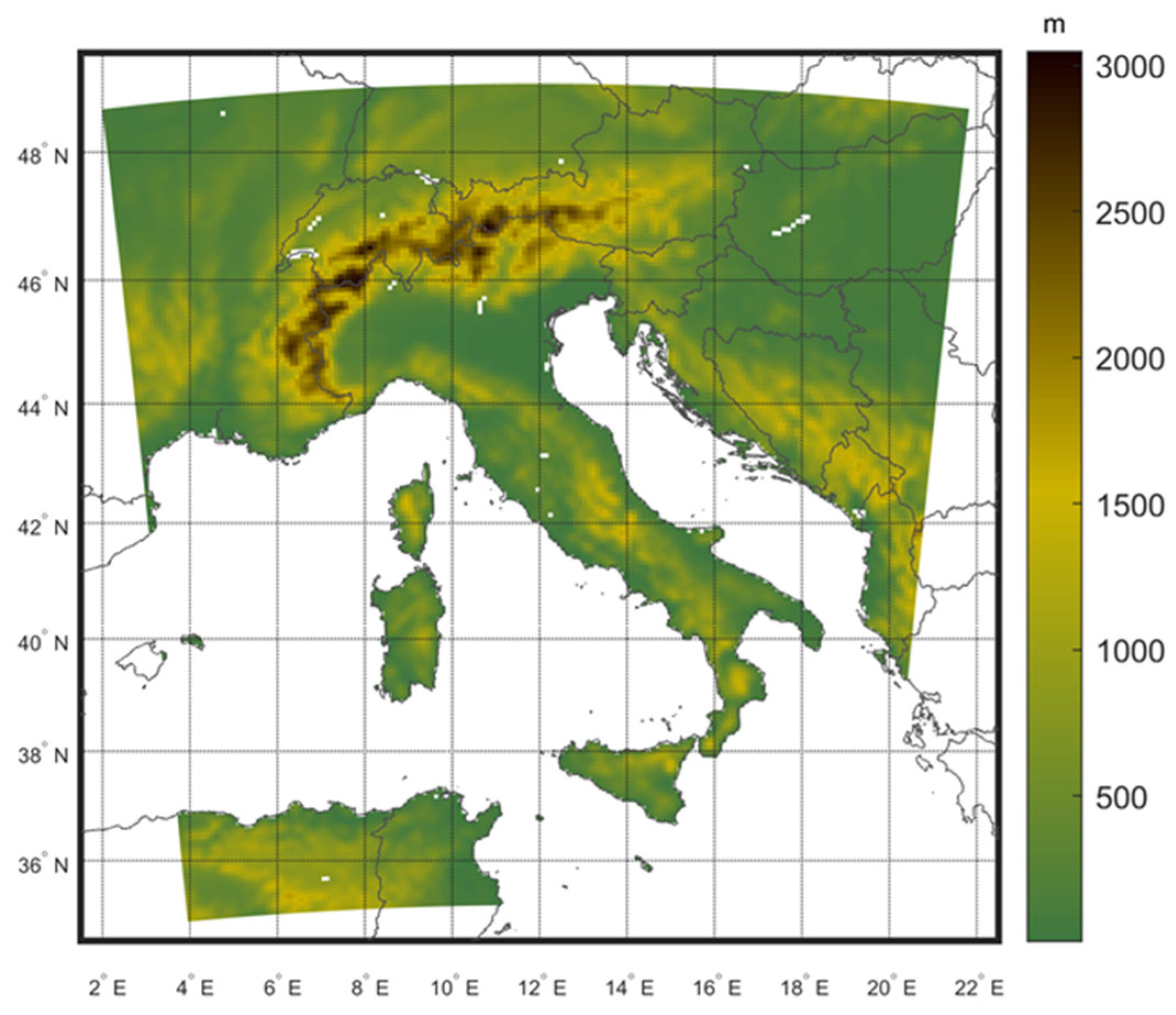
Figure 1. Orography of the computational domain at a spatial resolution of 0.0715° (about 8 km).
Atmosphere 16 00843 g001
Figure 2. Bias of 2 m mean temperature (°C) of ERA5- (a,c) and GCM EC-EARTH- (b,d) driven simulations at 0.0715° for DJF and JJA with respect to E-OBS, averaged over the period 1981–2010.
Atmosphere 16 00843 g002
Figure 3. Bias of total precipitation (mm/month) of ERA5- (a,c) and GCM EC-EARTH- (b,d) driven simulations at 0.0715° for DJF and JJA with respect to E-OBS, averaged over the period 1981–2010.
Atmosphere 16 00843 g003
Figure 4. Annual cycle of 2 m daily mean (T_2m), minimum (Tmin_2m), maximum temperature (Tmax_2m) (°C) and total precipitation (Tot_Prec) (mm/month) for Roma Fiumicino airport: EC-Earth-driven simulations at 0.0715° and 0.44° (CCLM8km and CCLM50km) and ERA5-driven simulation (CCLM8km_ERA5) against E-OBS and SCIA datasets, averaged over the period 1981–2010.
Atmosphere 16 00843 g004
Figure 5. Yearly time series (5-year running mean) of 2 m daily minimum, mean, maximum temperature (°C) and total precipitation (mm/year) of simulation at 0.0715° of resolution for Roma Fiumicino (nearest grid point).
Atmosphere 16 00843 g005
Figure 6. Time series of daily maximum and minimum T_2m over the periods considered (a,c) and corresponding mean power spectra obtained by FFT (b,d).
Atmosphere 16 00843 g006
Figure 7. Time series of daily total precipitation and 10 m wind speed over the periods considered (a,c) and corresponding mean power spectra obtained by FFT (b,d).
Atmosphere 16 00843 g007
Figure 8. Log–log plots of the relationship between L(k) and k for (a) Tmax_2m, (b) Tmin_2m, (c) Total precipitation and (d) 10 m wind speed, for the two periods considered.
Atmosphere 16 00843 g008
Table 1. BIAS values of temperature (°C) and precipitation (mm/month), averaged over the whole domain considered for the two seasons considered, for both simulations.
BIASERA5
DJF
ERA5
JJA
GCM
DJF
GCM
JJA
T_2m−0.78−0.33−1.01−2.44
Tmax_2m−1.51−0.35−1.80−2.58
Tmin_2m0.150.310.01−1.74
Total precipitation0.8010.332.835.66
Table 2. Values of the main periods recorded (in days) for the four variables considered.
Main Period (Days)T1T2T3
Tmax_2m365182121
Tmin_2m365182-
Total precipitation365182-
10 m Wind speed365182-
Table 3. Values of the fractal dimension for Tmax_2m, Tmin_2m, Total precipitation, and Wind speed, for the two periods considered.
Fractal Dimension1981–20102021–2050
Tmax_2m0.72230.7249
Tmin_2m0.70990.7139
Total precipitation0.90200.9028
Wind speed0.89600.8988
Disclaimer/Publisher’s Note: The statements, opinions and data contained in all publications are solely those of the individual author(s) and contributor(s) and not of MDPI and/or the editor(s). MDPI and/or the editor(s) disclaim responsibility for any injury to people or property resulting from any ideas, methods, instructions or products referred to in the content.