The Role of Air Mass Advection and Solar Radiation in Modulating Air Temperature Anomalies in Poland

Abstract

This study examines the roles of air mass advection and solar radiation in shaping daily air temperature anomalies in Warsaw, Poland, from 2008 to 2023. It integrates solar radiation data, HYSPLIT back-trajectories, air temperature measurements, and machine learning methods, which are key atmospheric factors contributing to temperature anomalies in different seasons. Radiation dominates during warm seasons, while advection-related geographic factors are more influential during winter. Increased solar radiation is observed across all seasons during high-positive temperature anomalies (exceeding two standard deviations). In contrast, cold anomalies in summer are accompanied by strong negative solar radiation anomalies (−136.3 W/m²), while winter cold events may still coincide with positive radiation anomalies (25.7 W/m²). Very slow circulation over Central Europe, which occurs twice as often in summer as in winter, leads to positive temperature (1.3 °C) and negative radiation (−2.1 W/m²) anomalies in summer and to negative temperature (−1.9 °C) anomalies and slightly positive radiation (0.3 W/m²) anomalies in winter. The seasonal variability in the spatial origin of air masses reflects shifts in synoptic-scale circulation patterns. These findings highlight the importance of considering the combined influence of radiative and advective processes in driving temperature extremes and their seasonal dynamics in mid-latitude climates.

1. Introduction

Climate change, driven largely by increasing concentrations of greenhouse gases (GHGs), continues to alter atmospheric processes and the Earth’s energy balance [1]. In addition to GHG-related warming, recent decades have seen notable shifts in the surface radiation budget, a phenomenon often referred to as global dimming and brightening [2,3]. These trends are particularly relevant in regions like Central Europe, where complex interactions between atmospheric circulation, cloud cover, aerosols, and surface properties play a key role in modulating the availability of solar radiation at the surface [4,5,6,7].

For example, the decline in aerosol emissions since the 1990s, associated with industrial transformation and air quality regulations, has contributed to increased surface solar radiation [8,9,10]. These changes affect not only the magnitude of solar energy received at the surface but also broader climatic processes such as the surface temperature, sensible and latent heat flux, and atmospheric stability [11,12]. In Central Europe and Poland, variability in the radiation budget over recent decades is characterized by both short-term fluctuations and long-term patterns [13]. Ref. [7] reported positive and statistically significant trends in the radiation budget in Poland on the Earth’s surface (1.5 ± 0.2 W/m²/10 year) in the last four decades.

Atmospheric circulation, alongside local radiation budget, plays a crucial role in shaping weather and climate patterns in the mid-latitudes [14,15]. Situated in Central Europe, Poland experiences significant weather variability driven by the passage of both low- and high-pressure systems [16]. The country’s climatic conditions are predominantly influenced by zonal (west–east) circulation patterns. Although less frequent, meridional (north–south) circulation events are associated with pronounced thermal anomalies. These circulation types not only determine the direction and characteristics of air mass advection but also have a significant impact on incoming solar radiation [17].

The combined effect of air mass advection and solar radiation is evident in the occurrence of large-scale temperature anomalies in Central Europe. Continental-scale thermal anomalies (CTAs), defined by significant deviations from long-term temperature averages, are often linked to specific circulation patterns that govern air mass advection and solar radiation exposure [18]. For instance, positive CTAs (warm anomalies) have increased in frequency, often associated with anticyclonic conditions that promote warm air advection and enhanced solar radiation [18,19]. Negative CTAs (cold anomalies) are linked to cold air mass advection under weakened zonal flow and reduced solar input due to cloudier conditions or shorter daylight in winter [18,20,21]. The impact of these combined factors varies seasonally and regionally within Central Europe. Winter cold anomalies are frequently caused by the advection of cold air masses, combined with limited solar radiation, while summer heatwaves result from warm air advection and strong solar heating under high-pressure systems [21,22]. The spatial extent and severity of anomalies depend on the persistence of circulation patterns and the origin and pathway of air masses [18,21].

Air temperature anomalies in Poland have shown significant variations in recent decades, often linked to both natural variability and anthropogenic factors. Long-term temperature records indicate an upward trend in annual mean temperatures, particularly since the 1980s, with notable warm periods observed in the 2000s [23]. These temperature increases have been accompanied by shifts in seasonal temperature patterns, with warmer winters and hotter summers becoming more frequent [24]. Extreme temperature anomalies have been observed to intensify under the influence of changing atmospheric circulation patterns, which modify the advection of warm and cold air masses [25]. The impact of these anomalies is particularly pronounced on agriculture, hydrology, and human health [26]. Additionally, air temperature anomalies in Poland are closely related to broader European-scale climate drivers, including changes in the North Atlantic Oscillation (NAO) and the Arctic Oscillation (AO), which influence the frequency and intensity of temperature extremes [27,28].

Understanding the combined effects of air mass advection and solar radiation is essential for interpreting temperature anomalies in Poland. The paper uniquely combines the effects of both air mass advection and solar radiation, alongside machine learning methods, to analyze daily near-surface air temperature anomalies in Warsaw, Poland, over a recent 15-year period (2008–2023), with particular attention to seasonal dependencies. Previous studies have often focused on either solar radiation or atmospheric circulation separately but rarely on their combined and seasonally differentiated roles in temperature anomalies. For our analysis, we used an extensive dataset, including data from The Hybrid Single-Particle Lagrangian Integrated Trajectory (HYSPLIT) simulations, ERA5 reanalysis, and the measurement data from the WXT520 Vaisala weather station, the CMP22 Kipp and Zonen pyranometer, and the NR Lite net radiometer. As a result, the presented study provides new insights into the drivers of temperature anomalies in mid-latitude urban settings, filling a gap left by previous studies that treated these factors in isolation or at broader spatial/temporal scales.

The paper is divided into several sections. Section 2 outlines the methodology, including a description of the data sources and processing. Section 3 provides insight into research results and is divided into six subsections. Section 3.1 is dedicated to the air temperature and radiation anomaly statistical analysis. Section 3.2 analyzes the influence of the air mass transport direction. Section 3.3 concentrates on radiation’s influence on temperature anomalies, while Section 3.4 presents the results of an investigation into the impact of advection on temperature anomalies. Section 3.5 concentrates on extreme episodes, and finally, Section 3.6 aims to identify key factors influencing temperature anomalies. In the discussion (Section 4), the presented findings and their implications are discussed, and the paper is summarized with the highlights of the obtained results in the conclusions (Section 5).

2. Materials and Methods

2.1. Data

2.1.1. Weather Data

In this study, we used observations from a research station in Warsaw, Poland, and numerical simulation data. Poland’s climate is classified as temperate and is characterized by a transitional nature between maritime (oceanic) and continental types [29]. This means that the climate is influenced both by moist, mild air masses from the Atlantic Ocean and by drier, more extreme air masses from the Eurasian interior, resulting in significant variability from year to year and region to region. Warsaw, the capital and largest city of Poland (about 1.8 million people, with an area of 517 km², is located in the east-central part of the country on the Vistula River, approximately 260 km from the Baltic Sea and about 300 km from the Carpathian Mountains. The University of Warsaw site (an urban station) is located on a rooftop (52.21° N, 20.98° E, 115 m a.m.s.l.).

Atmospheric observations were conducted using the WXT520 Vaisala (Helsinki, Finland) weather station. This is a compact, multi-parameter instrument that integrates multiple sensors into a single housing, allowing for the continuous, real-time monitoring of essential atmospheric variables. Wind is measured using an ultrasonic anemometer. Temperature and humidity are measured with a capacitive sensor, and pressure is measured using a silicon barometer. The WXT520 also includes a rain gauge based on acoustic detection, which is capable of estimating precipitation intensity and accumulation.

Downward shortwave radiation fluxes were measured using the CMP22 Kipp and Zonen (Delft, Netherlands) pyranometer. This instrument belongs to the highest classification (Secondary Standard) according to the ISO 9060 standard [30] and is characterized by high accuracy and long-term stability. The sensor is based on a thermopile detector and features a dual-glass-dome construction, which minimizes convective effects and ensures high spectral selectivity over the range of 0.2 to 3.6 $\mathsf{\mu }$m. The CMP22 provides a low non-linearity ($<\pm$0.2%) and a fast response time of less than 5 s (for 95% of the signal). The net radiation (shortwave plus longwave, downward minus upward fluxes) is measured using the NR Lite net radiometer (Kipp and Zonen). The NR Lite2 consists of a pair of thermopile detectors and dome-shaped optical elements that reduce wind sensitivity and contamination while covering a broad spectral range from approximately 0.2 to 100 $\mathsf{\mu }$m. The sensor provided reliable estimates of net radiation under most environmental conditions, with a response time of less than 20 s. The weather station collects data every 1 min, while the radiometers take measurements every 30 s. The instruments were calibrated and evaluated within the Poland-AOD network [31].

2.1.2. HYSPLIT

The HYbrid Single-Particle Lagrangian Integrated Trajectory (HYSPLIT) system [32] simulates backward or forward trajectories of air parcels, accounting for transport, dispersion, chemical transformations, and deposition [33]. A common application of HYSPLIT is back-trajectory analysis, which is used to determine the origin of air masses and establish source-receptor relationships [32]. HYSPLIT can be run using meteorological data from various sources. In this study, we used the Global Data Assimilation System (GDAS) data with 1° spatial and 3-h temporal resolution [34].

2.1.3. ERA5 Reanalysis

ERA5 is the fifth-generation reanalysis dataset produced by the European Centre for Medium-Range Weather Forecasts (ECMWF) for global climate and weather studies [35]. It combines model data with observations from around the world to create a globally complete and consistent dataset, providing hourly estimates of numerous atmospheric variables. ERA5 data is available from 1940 onwards and is provided on a regular latitude–longitude grid with a 0.25° spatial resolution [36]. For this study, we used temperature data from ERA5 dataset that contains hourly data on single levels, indicating the 2-meter air temperature [K] [37]. This value is calculated by interpolating between the lowest model level and the Earth’s surface, accounting for atmospheric conditions.

2.2. Data Processing

The study covers the period of 2008–2023. The analysis focuses on daily anomalies in air temperature and solar radiation, defined as the differences between daily mean values and the corresponding long-term daily means calculated over the entire observation period. Due to the fact that the autocorrelation function (for air temperature and radiation flux) has a significantly shorter range than one year, the entire dataset was divided into separate years, and the mean was calculated as the average over these individual realizations. To remove some fluctuation, the daily long-term mean values were filtered by using the running mean with a 5-day window. In addition, we defined days with significant air temperature anomalies as those when the anomaly exceeds 1 $\sigma$. HYSPLIT simulations were performed to generate 96-h back-trajectories for each day at 00:00 and 12:00 UTC, with the starting point set in Warsaw (Poland) at 500 m a.m.s.l. From the simulation results, we retrieved data on radiation, I [W/m²], and temperature, T [°C], in Warsaw and longitude–latitude coordinates of the back-trajectory points at 24, 48, 72, and 96 h. Next, the long-term mean temperature (T_mean) was calculated for each day of the year using a 5-day window. The same method was used to calculate I_mean. The difference between the HYSPLIT-derived temperature for Warsaw (T) and T_mean provided information on air temperature anomalies [°C]. The distance and azimuth were calculated for the starting point (Warsaw) and the endpoints of the back trajectories. To complete the dataset, ERA5 temperature data at 2 m were downloaded for the entire study period. Temperature values at 2 m were then retrieved for all trajectory points (24, 48, 72, and 96 h) from both the 00:00 and 12:00 UTC simulations. Using the obtained data, temperature advection at the surface was calculated as follows:

$$ad{v}_{\mathrm{surf}}=T_{\mathrm{point},2\mathrm{m}}-T_{\mathrm{Warsaw},\mathrm{surf}}$$

(1)

To account for short-term temperature fluctuations, the mean advection was calculated using two data points from the same day (00:00 and 12:00 UTC) and one from the following day (00:00 UTC on +1d). As a result, the mean advection was obtained for each day of the analyzed period on four trajectory timescales (24, 48, 72, and 96 h). Such quantities can also be interpreted as a change in air temperature during air mass transformation. However, due to the variability of the cloudy fraction along the back-trajectory, these quantities are also sensitive to the local weather conditions.

In the analysis, filtered cases of clear-sky and overcast conditions were utilized. The cloud-screening algorithm is described by [31]. For this purpose, the measured and simulated total solar fluxes are used. The measurements are then assumed to represent clear-sky conditions if the difference between the model (with optimal optical parameters) and the observations is smaller than the accepted threshold.

2.3. Random Forest Regressor Model

To assess the factors that play a dominant role in shaping temperature anomalies, we used machine learning methods, specifically the random forest (RF) regressor model [38]. Random forests consist of multiple decision trees, each built using values from a randomly generated vector that is independently sampled and identically distributed across all trees in the forest. They are effective tools known for their resistance to overfitting and their high accuracy in both classification and regression tasks [39].

For our simulations, we used the Scikit-Learn RandomForestRegressor with n_estimators = 800. The random_state value was set to 42. The model was run for two versions of the independent variables. The first set included solar radiation anomalies, longitude, and latitude, while the second one consisted of solar radiation anomalies, azimuths, and distance variables. All spatial variables were provided for the 48-h point on back trajectories. Calculations were performed for the entire year, as well as for each month. In all cases, we randomly split our dataset (random_state = 42) into training data (70%) and test data (30%). As a result, for the whole year, the training dataset contained 3774 points, while the test dataset had 1618 points. The number of points for a single month varied slightly. The model, trained on the training data, was then applied to the test dataset. Based on the set of variables (features), the RF Regressor model forecasts the air temperature anomaly [°C]. Finally, we estimate the impact of meteorological parameters for each month on air temperature anomaly, based on the features’ importance, according to the methodology previously described in [40].

3. Results

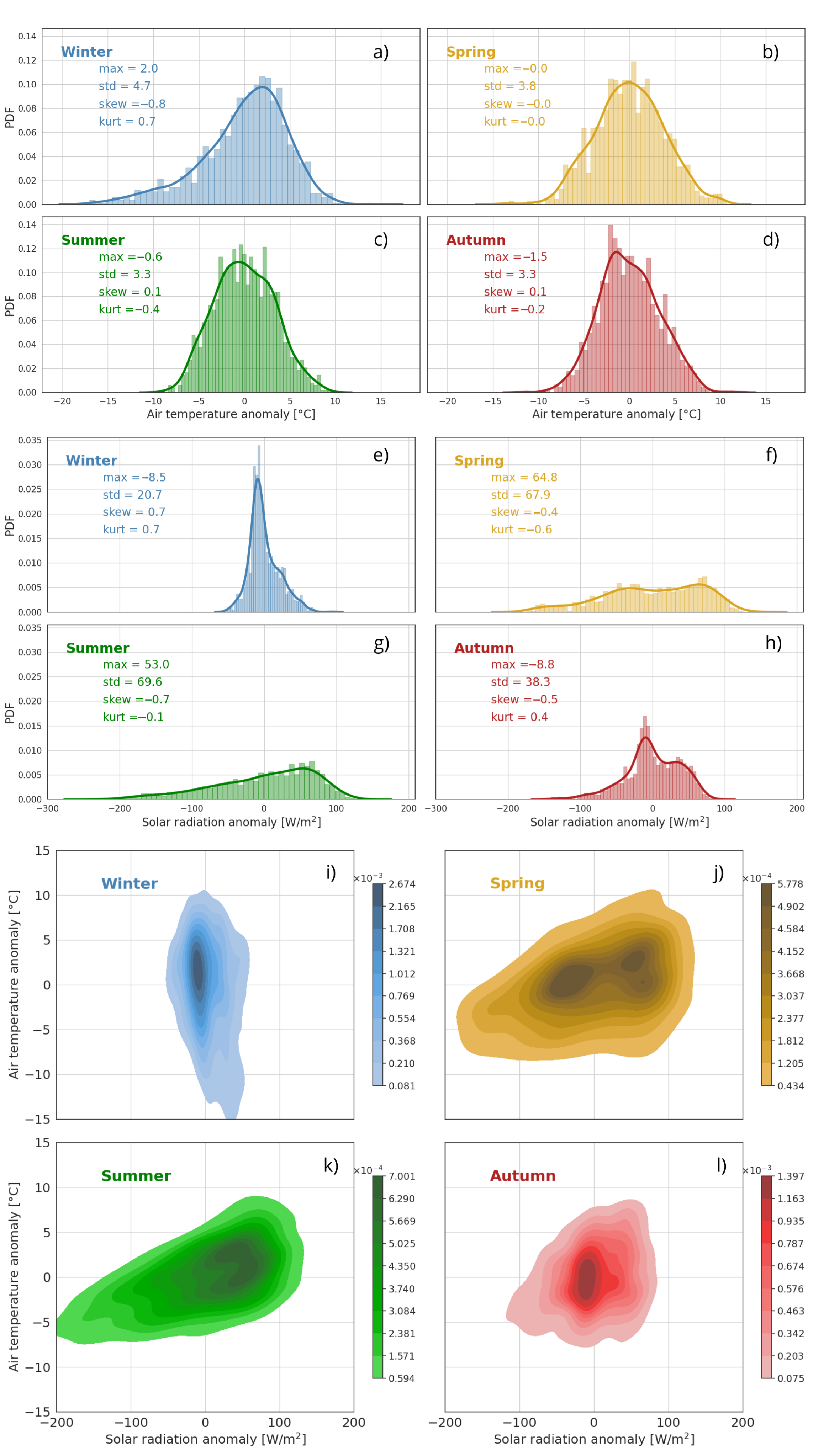
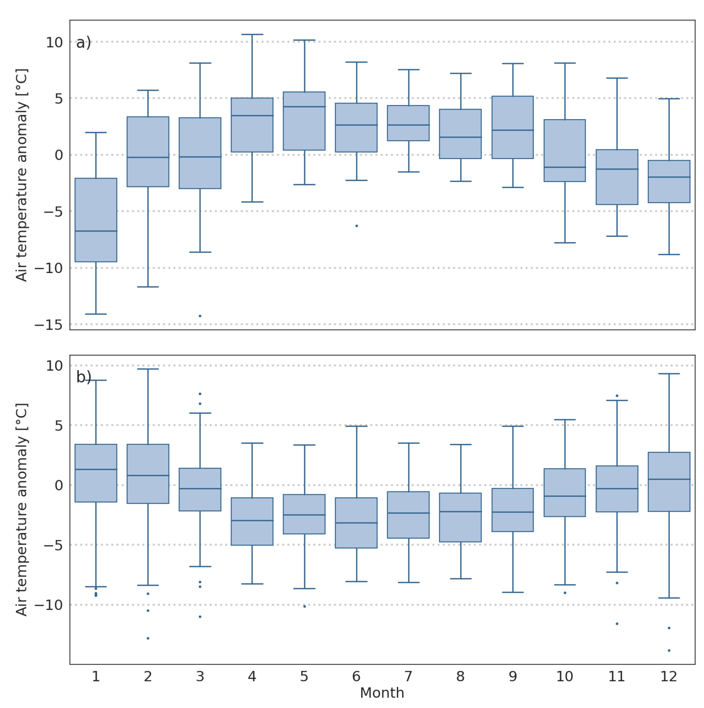
3.1. Statistical Assessment of Air Temperature and Solar Flux Anomalies

The probability distribution functions (pdfs) of the air temperature anomaly for the four seasons are presented in Figure 1a–d. The standard deviation is lowest during summer and autumn (around 3.3 °C) and highest in winter (4.7 °C). Skewness is nearly zero for spring (−0.04), negative (left tail) for winter (−0.8), and positive (right tail) for autumn (0.1) and summer (0.1). What is interesting is that, during winter, the most likely value of the temperature anomaly is 2.0 °C. At the same time, the significant asymmetry in the pdf indicates that cold events are more extreme than warm ones. In summer and autumn, the maximum of the pdf occurs for the negative anomaly (−0.6 and −1.5 °C). The pdf for spring is close to the normal distribution.

For the solar flux anomaly, the standard deviation varies between 20.7 W/m² for winter and 69.6 W/m² for summer. Significantly smaller standard deviations in autumn and winter are due to shorter daylight hours and a smaller relative difference between clear-sky and overcast conditions compared to spring and summer cases. The pdfs of radiation anomaly are significantly non-normal (Figure 1e–h). Skewness is positive only for winter (0.73). The negative tail corresponds with the overcast condition, while the positive corresponds with the low cloud cover or clear-sky condition. In particular, the maximum radiation flux is limited to the top of the atmosphere constraint. The two-modal distribution, especially in spring, can be explained by low and high cloud cover conditions. During summer, the most probable value of the solar flux anomaly is 53 W/m², while in spring, it is 65 W/m²; however, the flat pdf shows the second maximum close to −50 W/m². During winter and autumn, the most likely solar anomaly is close to −9 W/m².

The 2D pdfs for air temperature and solar radiation anomalies (Figure 1i–l) demonstrate a statistically significant relationship between the two variables in spring and summer. Negative radiation anomalies coincide with negative temperature anomalies, while positive solar flux anomalies correspond to warm episodes. During winter and autumn, the statistical relationship is very weak; however, in winter, it shows slightly opposite behavior. In addition, the 2D pdf for winter reveals a considerably greater spread in temperature anomalies compared to radiation anomalies.

Figure 2a presents the annual variability in the air temperature anomaly [°C] under clear-sky conditions. The results indicate that cloudless conditions translate into positive temperature anomalies during spring and summer. However, in winter, clear-sky conditions lead to negative temperature anomalies. This can be explained by the surface radiation budget. Between October and January, under clear-sky conditions, the net radiation flux becomes negative (Figure 3), leading to negative temperature anomalies. The negative net radiation during this period is due to the fact that the solar flux during short days cannot compensate for net (downward minus upward) infrared cooling (typically around −100 W/m²). During clear-sky conditions in February and March, the mean air temperature anomaly is negligible. In contrast, during May, clear-sky conditions led to an air temperature anomaly of about 4.0 °C.

Overcast conditions result in the opposite dependence (see Figure 2b). Slightly positive temperature anomalies (up to 1.4 °C) occur in winter (Dec–Feb), while negative ones are observed during the warm part of the year. During spring and summer, overcast conditions lead to air temperature anomalies as low as $-3$ °C.

The annual variability in surface net radiation (shortwave plus longwave; downward minus upward), shown in Figure 3, closely follows the seasonal changes in solar elevation (solar declination). The mean net radiation is slightly negative in January and December, close to zero in November, slightly positive in February, and significantly positive during the rest of the year. In late spring and summer, net radiation under clear-sky conditions is almost twice as high as under overcast conditions.

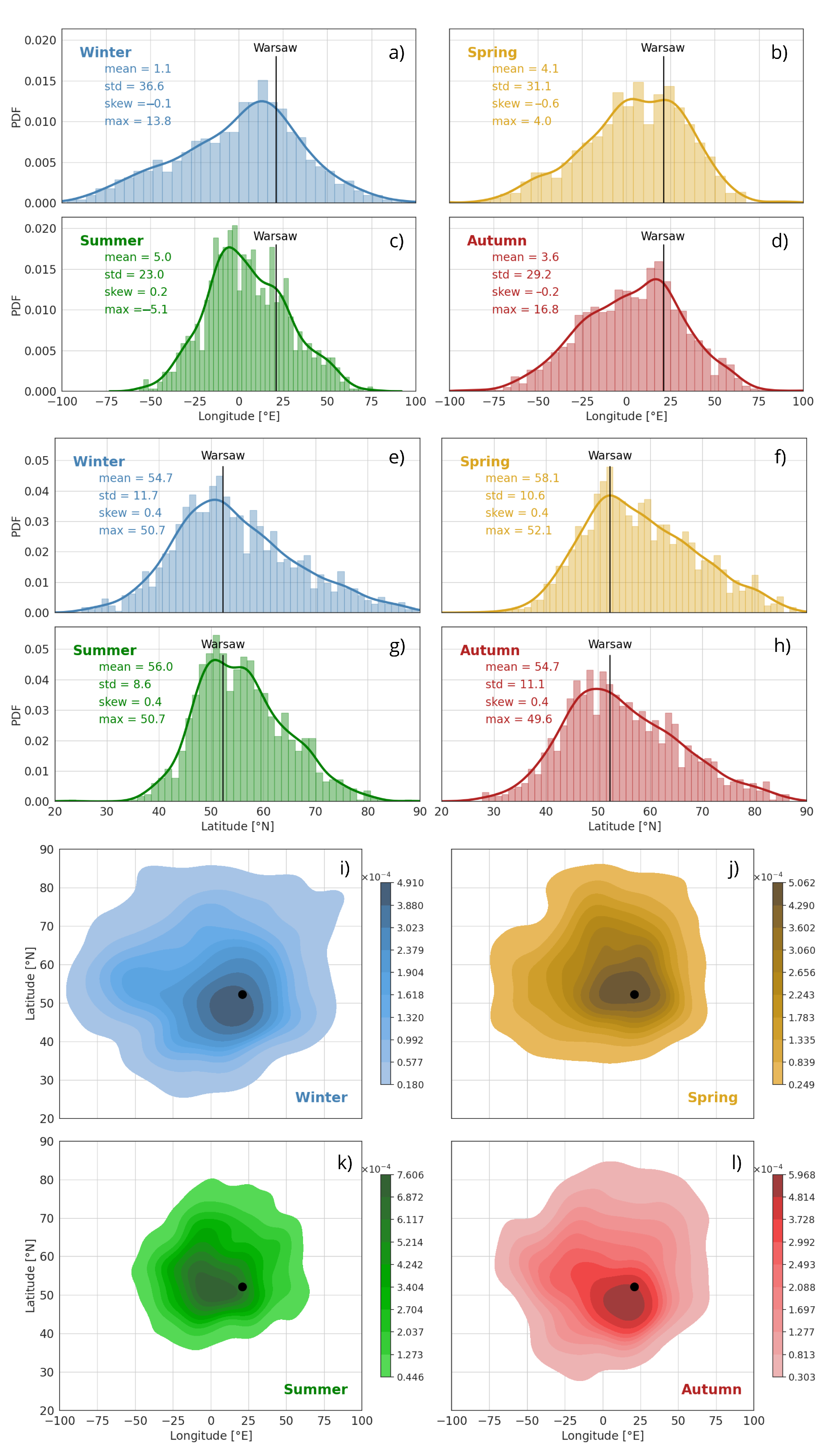
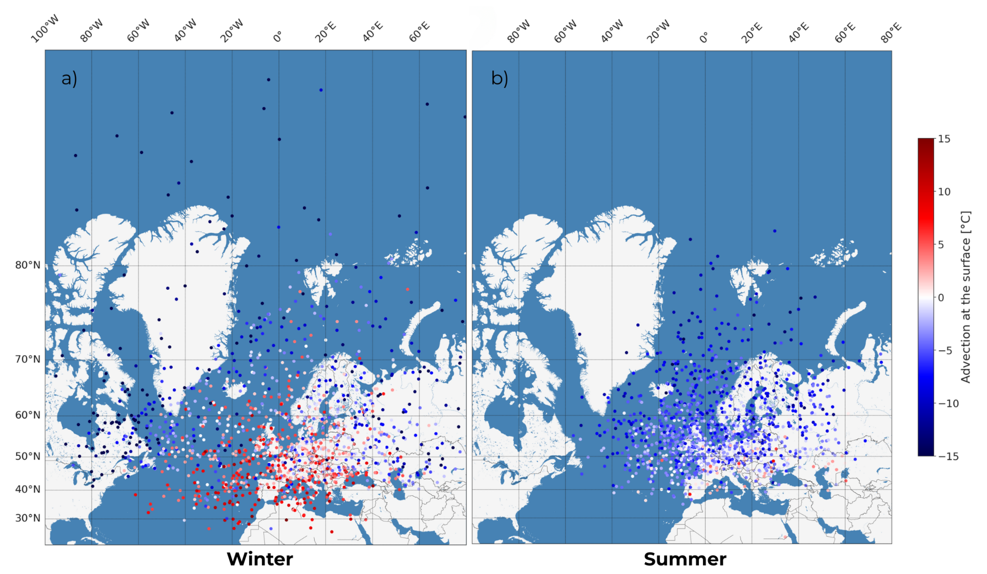
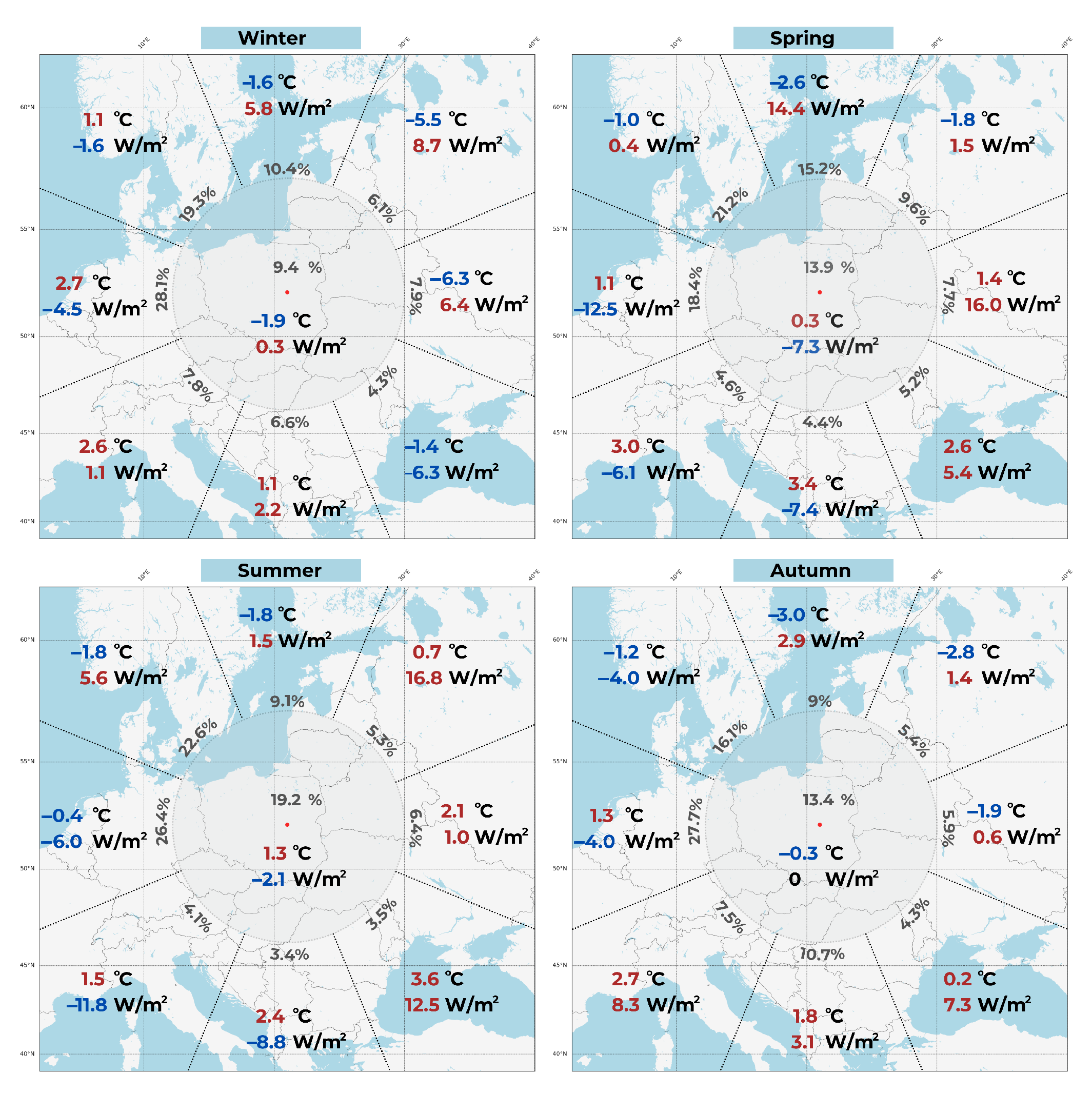
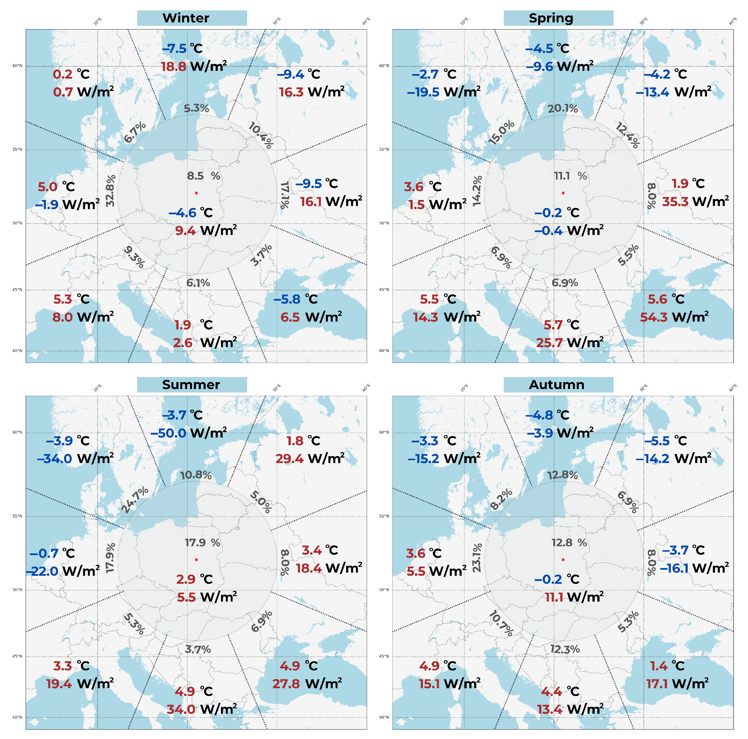
3.2. Influence of Air Mass Transport Direction on Temperature and Solar Radiation Anomalies Across Seasons

The dependence of air temperature [°C] and solar flux [W/m²] anomalies in Warsaw on the direction of air mass transport is depicted in Figure 4. The four diagrams correspond to the seasons in the order: winter, spring, summer, and autumn. For this analysis, 48-h back-trajectories ending in Warsaw at 500 a.m.s.l. were used. The entire domain was divided into nine regions. The central region covered an area within a 500 km radius of Warsaw, corresponding to very slow air mass transport over Central Europe. The remaining eight areas were defined by dividing the azimuthal plane into 45° sectors, centered on the geographical directions: N, NE, E, SE, S, SW, W, and NW. Similar diagrams but for air temperature anomaly higher than 1 $\sigma$ are shown in Figure 5.

Air masses from the central sector are observed on 9.4% of days in winter, nearly 14% in spring, 19% in summer, and 13% in autumn. These frequencies reflect the average velocity of air mass transport in mid-latitudes throughout the year. For this sector, the air temperature anomaly is significantly negative in winter (−1.9 °C) and slightly negative in autumn (−0.3 °C). In contrast, it is positive in summer (1.3 °C) and slightly positive in spring (0.3 °C). The solar radiation anomaly for this sector is negligible in winter and autumn (0.3 and 0 W/m², respectively) but becomes negative in spring (−7.3 W/m²) and summer (−2.1 W/m²), probably due to an increase in convection clouds developing. Significantly higher values are obtained for winter and summer when air temperature anomalies below 1 $\sigma$ are removed. During winter, the mean temperature anomaly in the central sector is −4.6 °C, while the radiation deviation 9.4 W/m² (Figure 5). In summer, the positive temperature anomaly is 2.9 °C, while radiation stands at 5.5 W/m².

During winter, over 55% of the cases correspond to SW, W, and NW (oceanic air masses) transport. These warm air masses are associated with a positive temperature anomaly (ranging from 1.1 to 2.7 °C) and a mostly negative radiation anomaly (from −2.6 to 1.1 W/m²). Conversely, during air mass transport from the E and NE, the temperature anomaly shows strongly negative values (−6.3 and −5.5 °C, respectively) accompanied by a positive radiation anomaly (6.4 and 8.7 W/m²). This pattern corresponds to anticyclonic circulation controlled by the East European or Siberian High. These results are consistence with [4], who reports a significant increase in the amount of surface solar radiation during air mass inflow from the north and east direction. Stronger positive radiation anomalies (between 16.1 and 18.8 W/m² for N, NE, and E sectors) are observed during significant temperature anomalies (Figure 5).

In spring, increased transport from the N is observed; however, the flow from NW and W dominates. Transport from NW, N, and NE reduces air temperature, ranging from −2.6 to −1.0 °C, while increasing solar flux from 0.4 to 14.4 W/m². This type of circulation is mostly observed in April and May as the advection of Arctic air from the north [41,42]. However, during days with a temperature anomaly higher than 1 $\sigma$, the radiation fluxes are above the mean value only for the easterly flow. During transport from N and NE, the negative radiation anomalies are observed, respectively, at −9.6 and −13.4 W/m². Warmer air masses are transported from the south (3.4 °C), but in this case, the solar flux is lower by 7.4 W/m². The most positive radiation anomaly is observed during transport from the east (16.0 W/m²) as a result of the reduction in cloud cover (in the continental dry air mass). For temperature anomalies above 1 $\sigma$, the radiation fluxes exceed the average value by 54.3 W/m² during SE flow.

In summer, only air mass transport from W, NW, and N reduces the air temperature by −0.4, −1.8, and −1.8 °C, respectively. The largest temperature anomaly is observed for flow from SE (3.6 °C) and S (2.4 °C); however, this type of circulation occurs on only 6.9% of days. A negative solar flux anomaly (ranging from −11.8 to −6.0 W/m²) is measured only during S, SW, and W transport, which accounts for approximately 35% of cases. The largest positive solar flux anomaly (16.8 W/m²) is observed for continental air masses transported from the NE. On such days, the mean temperature anomaly is slightly positive (0.7 °C). However, during a high temperature anomaly (above 1$\sigma$), the radiation flux anomaly is positive for NE, E, SE, S, and SW flow and strongly negative at N, NW, and W. This shows that transport of air mass from W to N sector brings more cloud and lower temperature. The advection of air masses from other directions results in increased temperature and solar radiation.

In autumn, there is a relatively high frequency of air mass transport from the southern sector (10.7%), similar to that from the north (9%). The most frequent transport occurs from W and NW, covering almost 34% cases. The highest positive temperature anomalies are observed for SW (2.7 °C) and S (1.8 °C) flows (mostly associated with Azorian High), coinciding with a positive radiation flux anomaly (3.1 W/m² for S and 8.3 W/m² for SW). Strong temperature reductions are recorded during N (−3.0 °C) and NE (−2.8 °C) transport, which are also associated with a positive radiation anomaly (2.9 and 1.4 W/m², respectively). Only during W and NW circulation, the radiation anomaly is negative (−4.0 W/m²). For significant temperature anomaly, the negative radiation anomaly is observed only during W and NW flow.

Figure 6 (adjusted figures numbering) shows the spatial distribution of the ending points of back-trajectories with temperature anomaly in Warsaw during winter and summer. During winter, negative anomalies are observed for back-trajectories that end in Poland or the eastern direction, while positive values are obtained for air mass transported from the North Sea and high latitudes. In summer, the positive anomaly is observed when back-trajectories end in the east and south directions from Warsaw, while negative during transport from the west, west-north, and north directions.

Table 1. Spearman correlation coefficient between air temperature [°C] and solar flux anomaly [W/m²] for nine defined sectors (see Figure 4). The values given in brackets are statistically insignificant at a 95% confidence level. Results are given for the full dataset (columns all) and for the significant anomalies (above 1$\sigma$).

Direction	Winter		Spring		Summer		Autumn
	all	>1 $\mathbf{\sigma }$	all	>1 $\mathbf{\sigma }$	all	>1 $\mathbf{\sigma }$	all	>1 $\mathbf{\sigma }$
<500 km	−0.38	−0.63	0.59	0.63	0.58	0.76	0.40	0.58
N	−0.16	(−0.24)	0.43	(0.17)	0.60	0.55	(0.12)	(0.09)
NE	−0.36	−0.42	0.38	(0.18)	0.51	0.66	0.35	(0.1)
E	−0.60	−0.43	0.44	0.65	0.69	0.84	0.30	(0.26)
SE	−0.35	(−0.45)	0.73	(0.26)	0.70	0.54	0.33	0.49
S	(0.11)	(−0.05)	0.67	(0.14)	0.80	(0.44)	0.41	0.5
SW	(−0.08)	(−0.08)	0.52	0.47	0.84	0.58	0.35	0.62
W	(0.03)	(−0.08)	0.36	0.52	0.57	0.82	0.27	(0.18)
NW	−0.16	(−0.33)	0.39	0.55	0.57	0.55	0.13	0.33
Mean	−0.24	−0.3	0.50	0.4	0.65	0.64	0.29	0.35

shows the Spearman correlation coefficient for air temperature and solar flux anomalies for each season and all transport sectors. Negative values are observed only in winter. For transport from NE, E, and SE, a moderate negative correlation coefficient (ranging from −0.6 to −0.35) indicates that negative temperature anomalies are associated with continental air masses under cloudless conditions. In autumn, the correlation coefficients are positive for all sectors, but their values do not exceed 0.42. In spring and summer, the correlation coefficient is significantly higher. During spring, particularly for transport from S and SE, the correlation coefficient reaches 0.67–0.73. For other flow directions, the correlation coefficient is lower, ranging from 0.36 to 0.59. The statistical relationship between air temperature and solar flux is strongest in summer. The Spearman correlation coefficient reaches 0.84 for SW transport and 0.8 for S transport, and it is around 0.7 for E and SE transport.

The Spearman correlation coefficient between temperature anomalies and solar flux anomalies and the position of back-trajectories ending in Warsaw (at 500 m a.m.s.l.) is shown in Figure 7. Significant correlation coefficients (around 0.5) between air temperature and solar flux in Warsaw were obtained between April and September. A negative correlation (−0.3) was calculated for January, indicating that clear-sky conditions are associated with cold anomalies. For the rest of the autumn and winter months, the statistical relationship between air temperature anomalies and solar radiation is very weak.

In the case of temperature anomalies and the longitude of back-trajectory points, the correlation coefficient is negative from January to March and from September to December, while it is positive between April and August (Figure 7b). Positive values indicate that a shift of the endpoint of an air mass towards the east (more continental air mass) corresponds to warm episodes, while a shift towards the west (more marine air mass) brings colder air masses. A negative correlation coefficient reflects the opposite behavior, which is typical for autumn and winter. However, the absolute values of the correlation coefficient during spring and summer (up to 0.3) are lower than those observed in autumn and winter (up to −0.6).

The Spearman correlation coefficient between air temperature anomalies and the latitude of back-trajectories is negative for all months (Figure 7c). This result indicates an obvious fact that air mass transport from the north leads to colder conditions, while transport from the south results in warmer conditions. Significant correlation values are observed in spring (March and April, up to −0.55) and late summer/autumn (August, September, and October, up to −0.65). Between May and July, the correlation coefficient is relatively small (up to −0.35), indicating a minor effect of the direction of the meridional transport on the temperature anomalies in Warsaw.

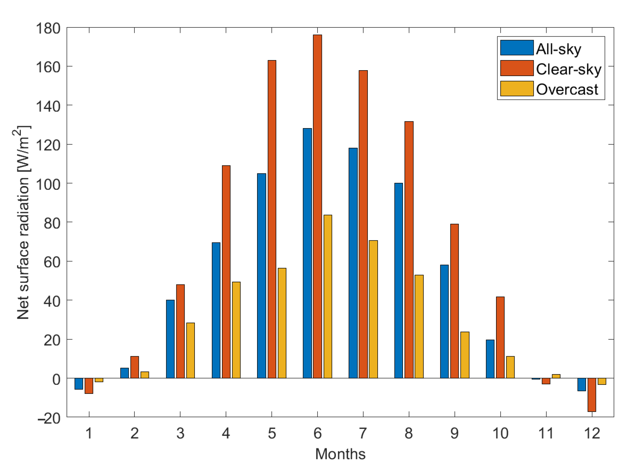
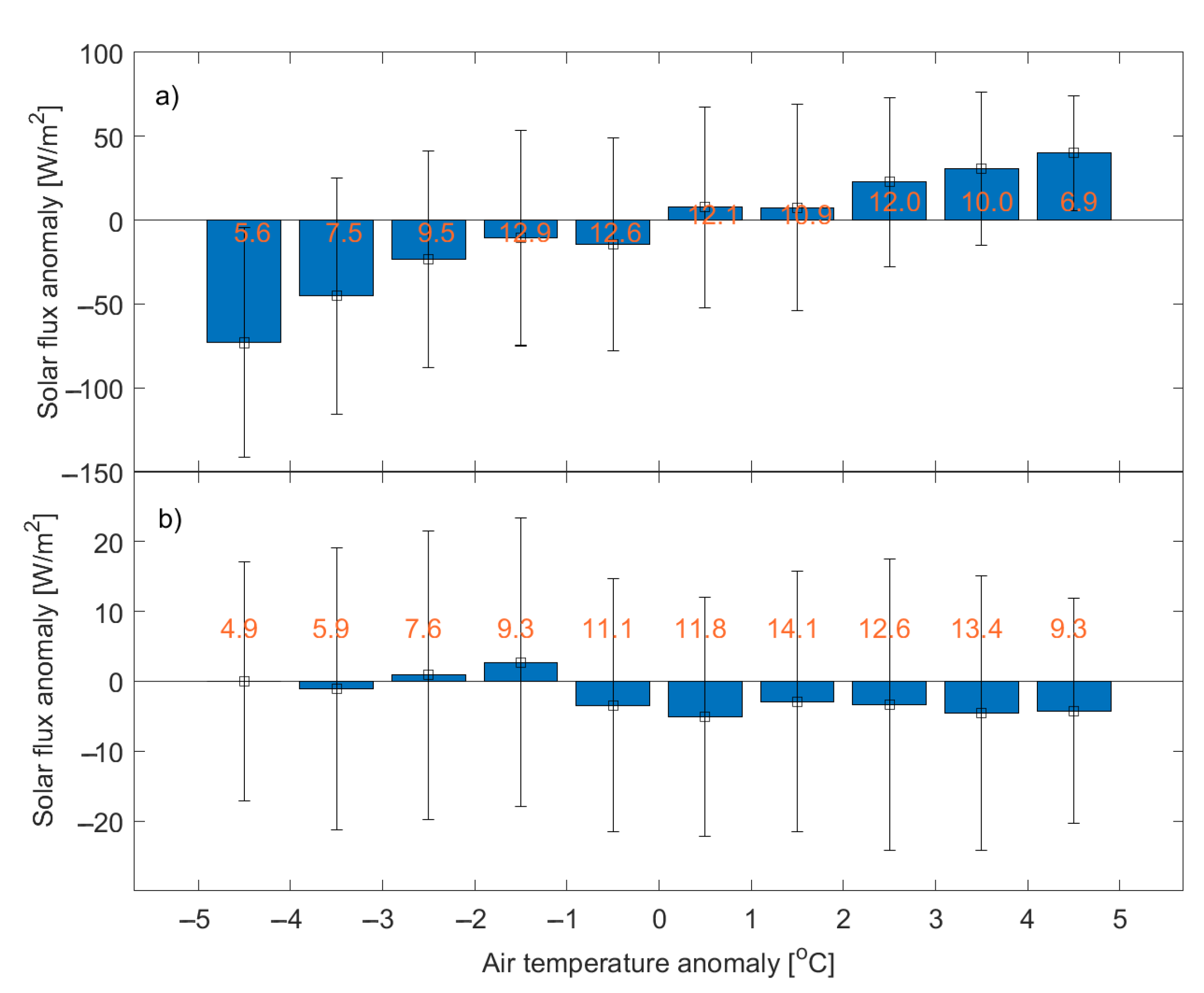
3.3. Radiation-Driven Temperature Anomalies in Winter and Summer

A systematic plot (Figure 8a) illustrates the relationship between air temperature and solar flux anomalies during summer. There is clear evidence that cold anomalies are associated with a reduction in solar flux, while warm episodes coincide with an increase in surface solar radiation. For example, a temperature anomaly in the range of 4–5 °C is observed on days when the solar flux anomaly is approximately 40 W/m². Conversely, during cold anomalies (−4 to −5 °C), the solar flux decreases by an average of 70 W/m². For small temperature anomalies (ranging from −2 to 2 °C), the radiation anomaly remains below ±15 W/m². In contrast, during winter (Figure 8b), the effect of solar radiation on air temperature is rather small. However, there is a systematic reduction in radiation during hot episodes (up to −5 W/m²), which must correspond to the advection of warm and wet air masses and cloudy conditions. For cold episodes, the radiation anomalies are rather negligible.

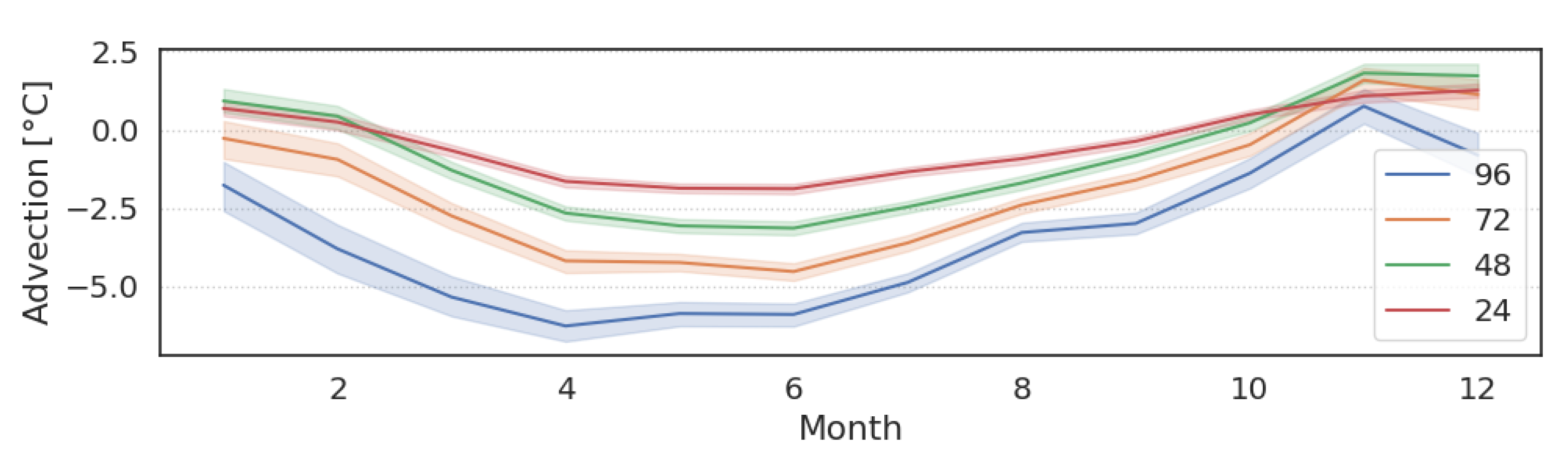
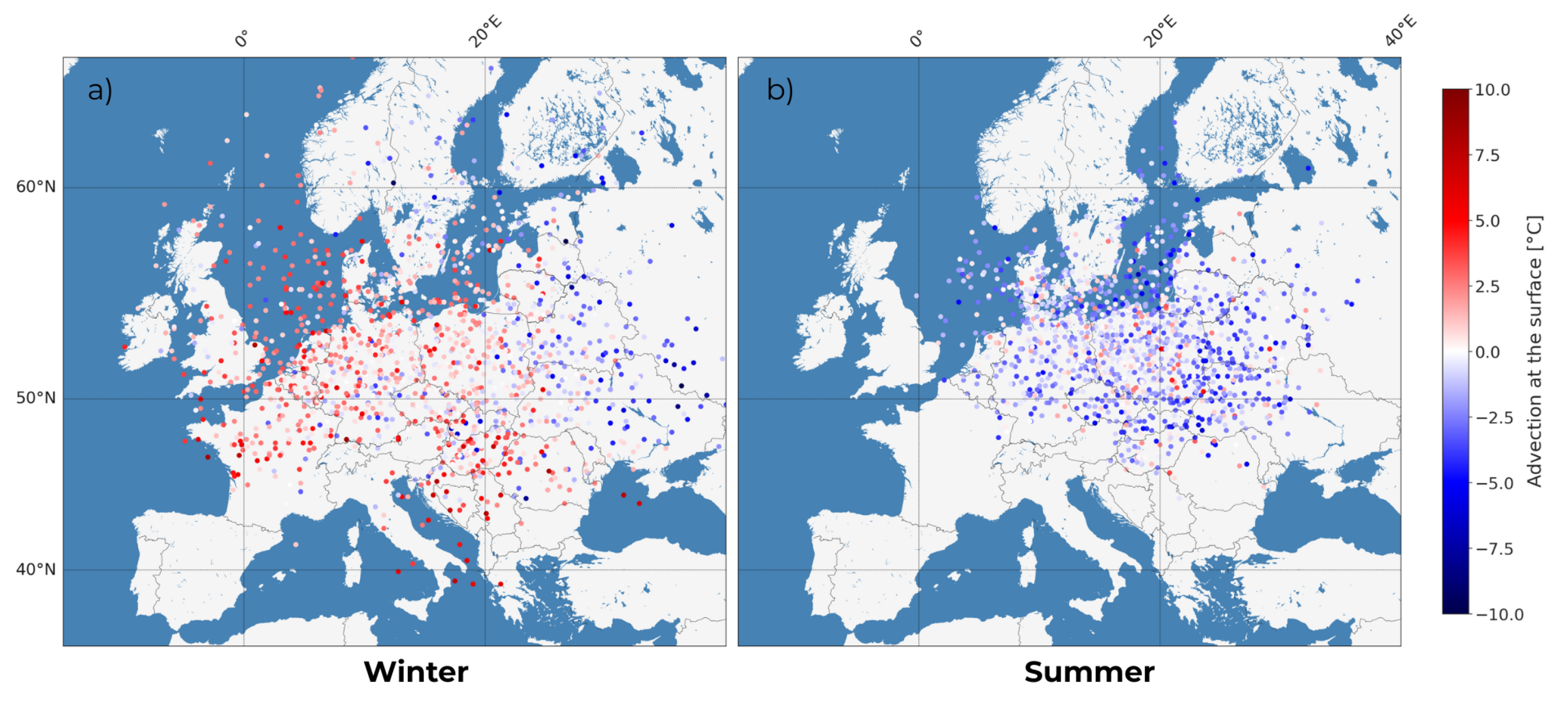
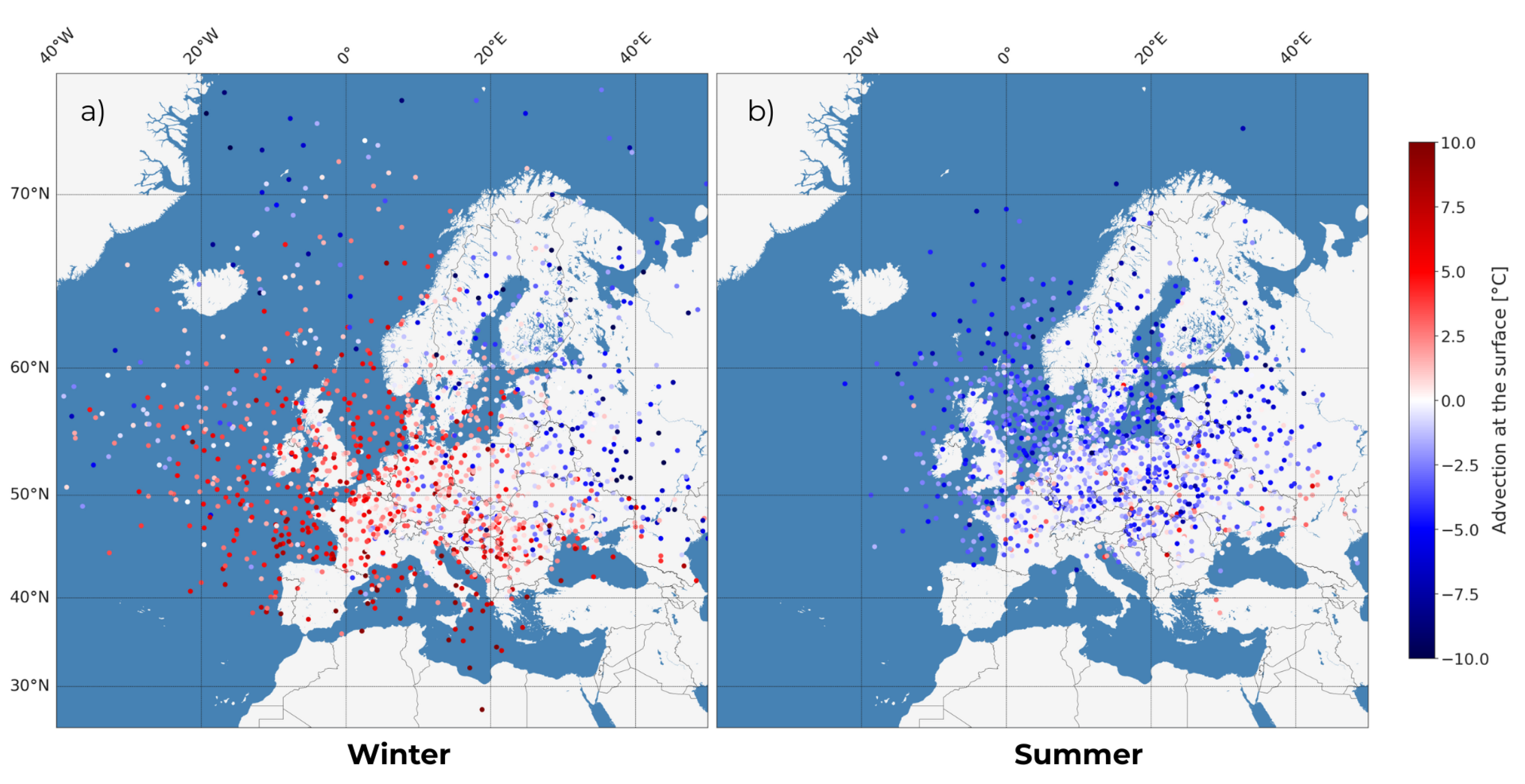
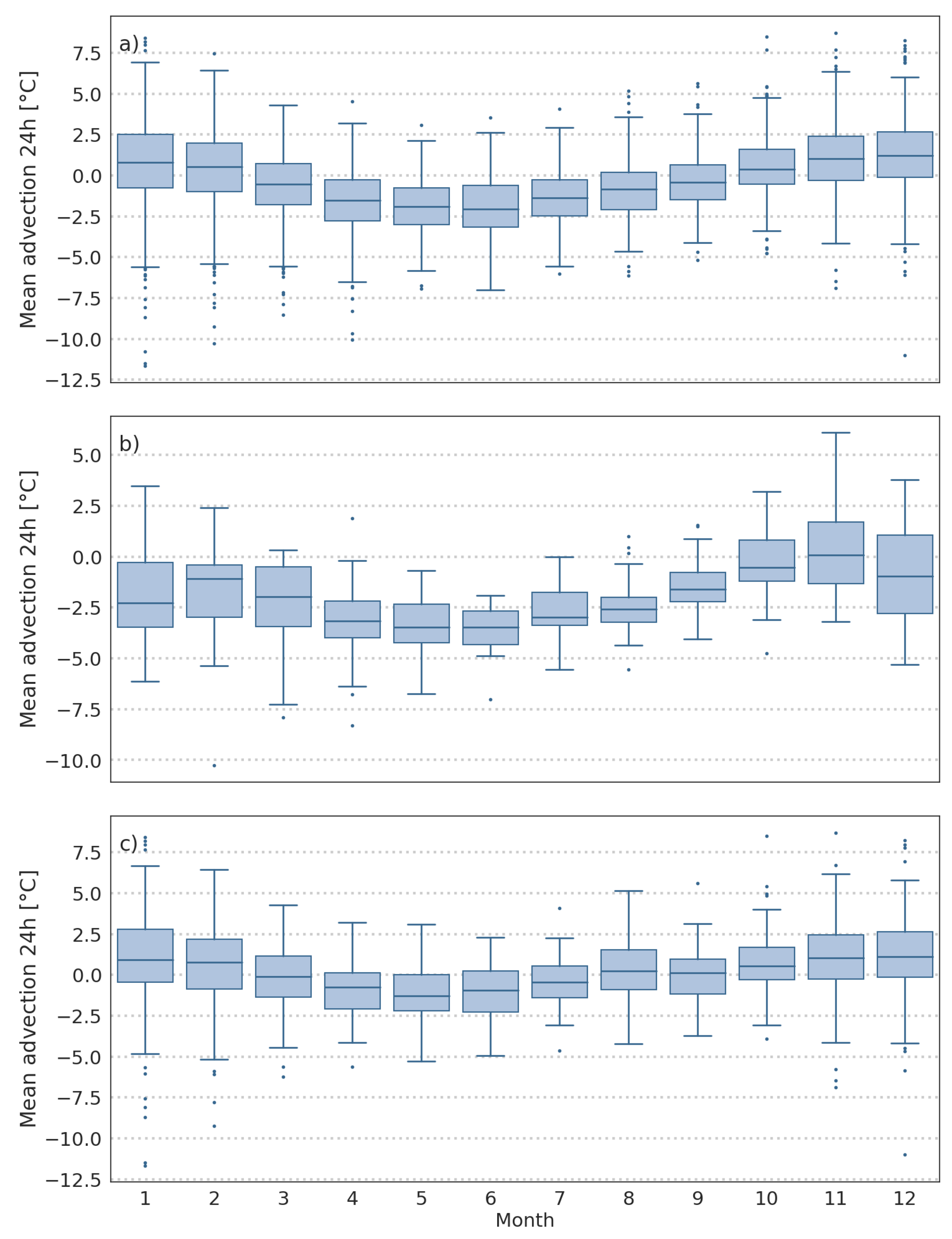
3.4. Impact of Advection on Temperature Anomaly for Different Seasons

Table 2. Descriptive statistics (mean, standard deviation, skewness, and kurtosis) of the mean 24-h advection at the surface [°C] for different sky conditions across seasons.

		Winter	Spring	Summer	Autumn	Annual
All cases	Mean	0.7	−1.4	−1.4	0.4	−0.4
	Std	2.6	2.0	1.8	1.9	2.1
	Skew	−0.6	−0.3	0.1	0.4	−0.1
	Kurt	1.8	0.5	0.0	1.0	0.8
Clear sky	Mean	−1.5	−3.0	−2.9	−0.6	−2.0
	Std	2.8	1.9	1.4	1.8	2.0
	Skew	−0.4	−0.3	0.3	0.9	0.1
	Kurt	0.7	0.0	1.0	1.2	7.3
Overcast	Mean	0.9	−0.6	−0.3	0.7	0.2
	Std	2.6	1.8	1.8	1.9	2.0
	Skew	−0.7	−0.1	0.2	0.2	−0.1
	Kurt	2.7	0.1	0.4	1.6	1.2

shows statistics of air temperature advection between Warsaw and the site defined by a 24 h back-trajectory (see Equation (1)) at 500 m for all seasons and all cases, clear-sky, and overcast conditions. The mean advection is positive (transport of warm air masses) in winter (0.7 °C) and autumn (0.4 °C) and negative (transport of cold air masses) in spring and summer (−1.4 °C) as a result of the net radiation budget at the Earth’s surface. During months with a high positive net radiation flux, cold air masses contribute to balancing the energy budget at the surface layer. Advection during clear-sky conditions brings colder air masses in all seasons. In spring and summer, air mass transport towards Warsaw increases air temperature by approximately 3 °C. In winter and autumn, the temperature changes by 1.5 °C and 0.6 °C, respectively. During cloudy conditions, the temperature change is significantly lower. Cold advection is observed in spring (−0.6 °C) and summer (−0.3 °C), while warm advection occurs in winter (0.9 °C) and autumn (0.7 °C).

Figure 9 shows a box-whisker plot for the monthly mean 24-h advection based on HYSPLIT and ERA5 reanalysis data. For all data (panel a), the warm advection is observed only in January and is almost zero in November, December, and February. The coldest advection is observed in May and June (−1.9 °C), which coincides with an increase in the north flow frequency (Figure 4) and also with a maximum of net radiation at the surface (Figure 3). Thus, the positive radiation budget at the surface is partly balanced by the cold air mass advection and partly by sensible and latent heat flux to the atmosphere. During clear-sky conditions, the mean advection is more negative to compensate for the more positive radiation net flux. Only during November, the mean temperature advection is close to zero, while in June, it is about −3.6 °C. In contrast, the mean advection is shifted towards positive values during overcast conditions. The difference between winter and spring/summer months is also visible in the largest spread of temperature advection during the cold season compared to the warm one. The annual variability in the surface air advection [°C] for different time points on back-trajectories is presented in Figure A2 in Appendix A. Longer back-trajectories almost always translate into colder advection (see also Figure A3, Figure A4 and Figure A5).

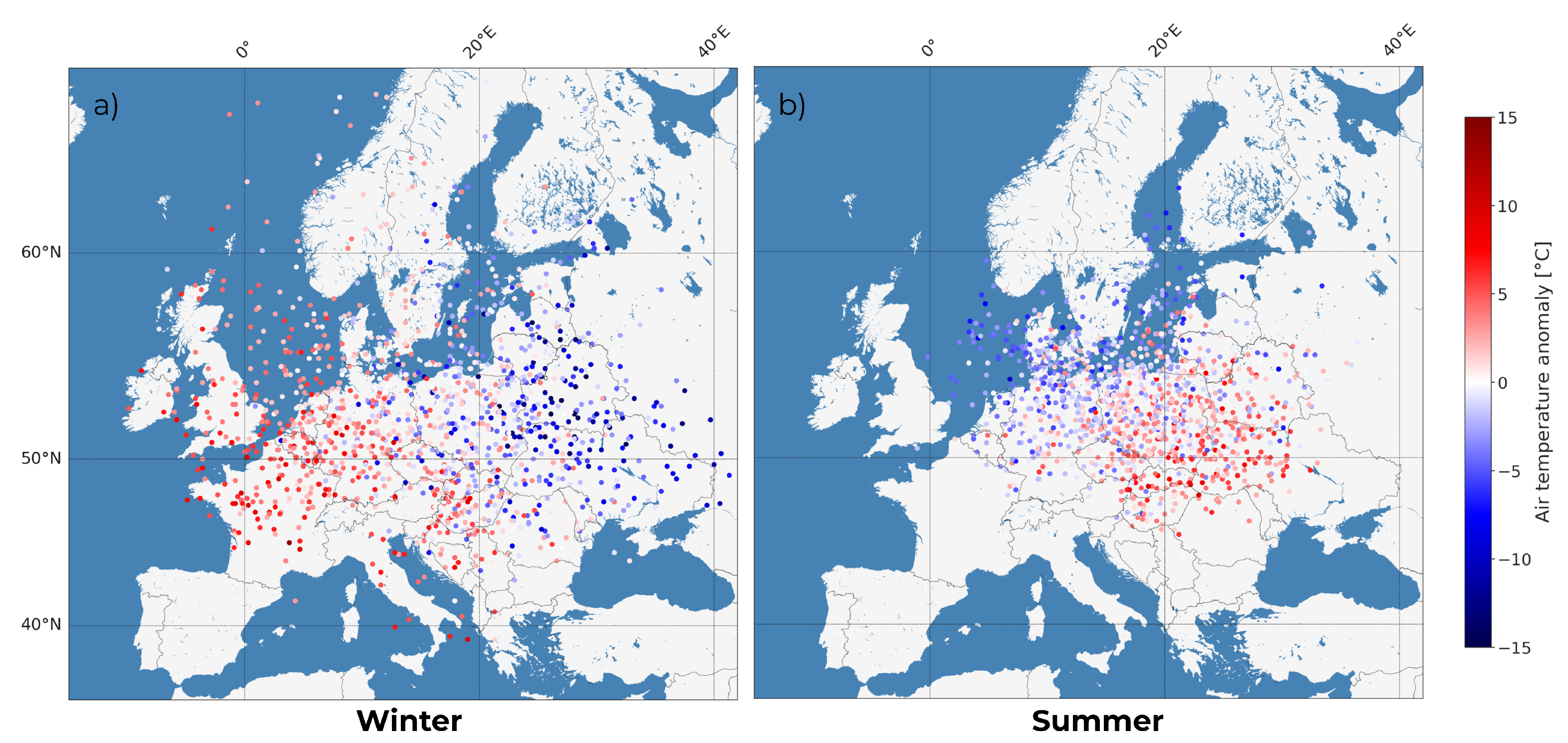
3.5. Extreme Warm and Cold Episodes

During extreme cold and warm episodes, defined as temperature anomalies exceeding 2$\sigma$ (two standard deviations), the solar flux anomaly is statistically significant in all seasons (see

Table 3. Mean and standard deviation of solar radiation anomaly [W/m²] and position anomaly (latitude and longitude) of 48 h back-trajectories ended in Warsaw at 500 m a.m.s.l. during extreme temperature episodes (mean daily absolute temperature anomaly above 2$\sigma$).

		Winter	Spring	Summer	Autumn
Radiation	−2$\sigma$	25.7 ± 19.5	−4.9 ± 70.3	−136.3 ± 57.6	−13.5 ± 44.0
	+2$\sigma$	6.1 ± 20.6	48.1 ± 40.4	64.3 ± 21.5	35.2 ± 22.5
Longitude	−2$\sigma$	22.2 ± 11.2	16.7 ± 9.9	−0.3 ± 13.3	19.8 ± 10.2
	+2$\sigma$	−10.5 ± 11.0	1.3 ± 11.9	11.2 ± 8.4	0.3 ± 13.0
Latitude	−2$\sigma$	1.2 ± 4.7	5.2 ± 6.1	6.5 ± 5.2	4.4 ± 5.0
	+2$\sigma$	−7.7 ± 3.0	−8.7 ± 2.9	−4.1 ± 3.6	−7.8 ± 4.7

). For instance, the mean solar flux anomaly during extremely warm days is 6.1 (19%) ± 20.6, 48.1 (29%) ± 40.4, 64.3 (28%) ± 21.5, and 35.2 (45%) ± 22.5 W/m², in winter, spring, summer, and autumn, respectively. Extreme cold days are associated with a strong positive solar anomaly in winter (25.7 (81%) ± 19.5 W/m²), relatively small negative anomalies in spring (−4.9 (3%) ± 70.3 W/m²) and autumn (−13.5 (17%) ± 40.0 W/m²), and a pronounced negative anomaly in summer (−136.3 (60%) ± 57.6 W/m²). The different radiation anomaly during cold episodes in winter is related to clear-sky conditions (see Figure 3), leading to more negative net radiation at the surface.

Regarding air mass trajectories, during strong positive temperature anomalies in winter, the back-trajectories shift by 10.5° westward and 7.7° southward, while in summer, they shift 11.2° eastward and 4.1° southward. In spring and autumn, significant shifts in back-trajectories are observed only in the meridional (north–south) direction: −8.7° in spring and −7.8° in autumn. For extreme cold episodes, the back-trajectories show a substantial eastward shift (22.2° in winter, 16.7° in spring, and 19.8° in autumn) and a consistent southward shift ranging from 7.7° to 8.7°. Only in summer, the shifts are more moderate, with a slight southward displacement (4.1°) and negligible zonal (east–west) movement.

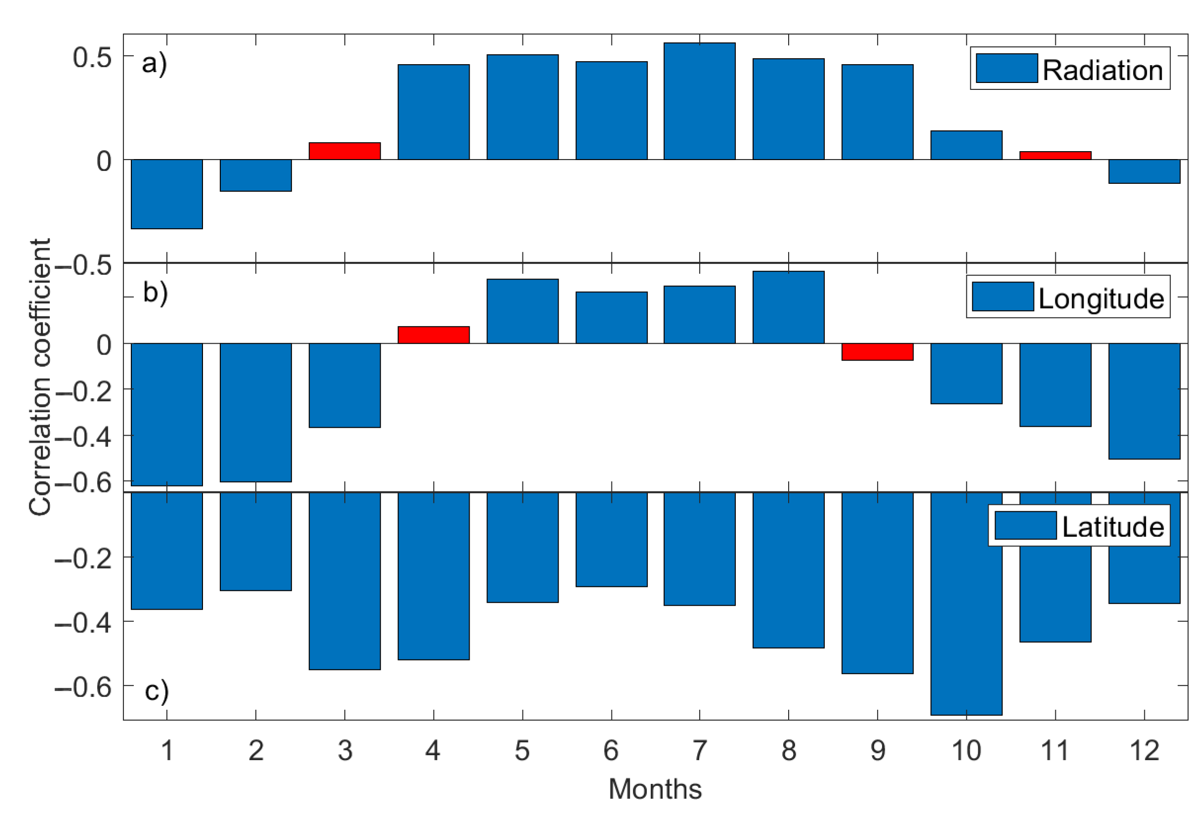
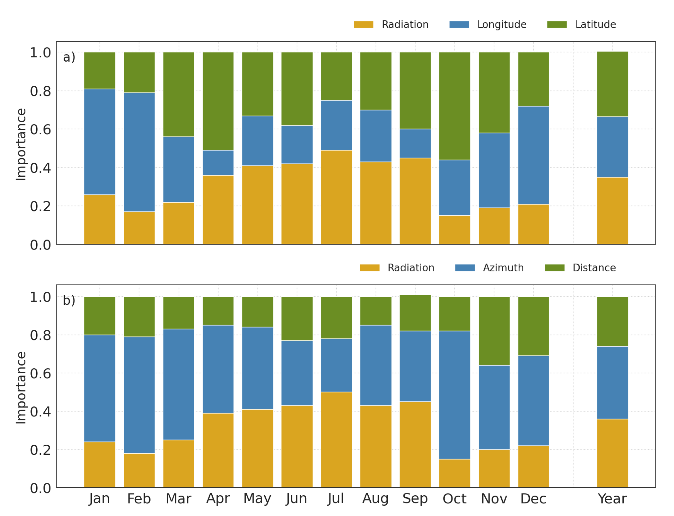
3.6. Identification of Key Factors Influencing Temperature Anomalies

To estimate the impact of meteorological parameters for each month on air temperature anomalies, the RF machine learning model was used. The model was run with two versions of the feature set. In the first one, the anomaly of solar radiation, longitude, and latitude of 48 h back-trajectories’ positions were set. In the second case, instead of longitude and latitude, the back-trajectory distance and azimuth were used.

Table 4. $R^2$ coefficient of determination of RF machine learning model, given for two sets of independent variables, (i) the solar radiation anomaly, longitude, and latitude and (ii) the solar radiation anomaly, azimuth, and distance.

	R2 Score
	Jan	Feb	Mar	Apr	May	Jun	Jul	Aug	Sep	Oct	Nov	Dec	Year
Lon, Lat	0.61	0.58	0.38	0.4	0.57	0.52	0.53	0.56	0.58	0.36	0.53	0.35	0.31
Az, Dist	0.61	0.62	0.39	0.44	0.56	0.51	0.52	0.54	0.53	0.35	0.51	0.35	0.31

shows the R² score, which is a statistical metric that quantifies the proportion of variance in the dependent variable that is accounted for with the independent variable in a regression model. This parameter changes from 0.35 to 0.61 in the first case and from 0.35 to 0.62 in the second case. When the model is run without monthly separation, lower values of R² (0.35) are obtained.

Figure 10 shows two stacked bar charts illustrating the importance of various parameters influencing air temperature anomalies in Warsaw regarding the random forests model. Each bar represents a different month of the year, with the final bar on the right summarizing the yearly importance of the parameters. In panel (a), the importance of three parameters—the solar radiation (yellow), longitude (blue), and latitude (green) of the 48 h back-trajectory—is depicted. The results indicate that the position of the air mass (longitude and latitude) is the dominant factor influencing temperature anomalies, while solar radiation plays a secondary role. However, the importance of these parameters varies, depending on the season. During winter, longitude and latitude play a more significant role, likely due to lower solar radiation levels and the impact of atmospheric circulation (advection). In contrast, during summer, solar radiation becomes more dominant (up to 0.5).

Spring and autumn show a more balanced contribution among the parameters, indicating transitional climatic influences that combine horizontal advection and solar radiation factors. What is interesting in March and April, as well as in September and October, is that the meridional transport (latitude) is more important than the zonal (longitude). The opposite behavior is observed in winter (December–January), when the zonal transport is more important than the meridional flow.

Similar results were obtained for solar radiation (yellow), the air mass azimuth angle (blue), and distance (green). The findings suggest that the azimuth is the most influential parameter (especially during winter and autumn), followed by solar radiation and distance.

The observed monthly fluctuations suggest that different mechanisms drive temperature anomalies, depending on the season. These findings underscore the importance of considering multiple parameters when analyzing climate variability in urban environments. We found that the Spearman correlation coefficient between air temperature anomaly and back trajectory distance and mean u and v wind component changes significantly with the season (

Table 5. Spearman correlation coefficient between air temperature anomaly and zonal (U-wind) and meridional (V-wind) wind speed and 48 h distance of back-trajectories ended in Warsaw at 500 m a.m.s.l. (U-wind and V-wind were calculated based on the HYSPLIT data).

	Correlation Coefficient
	Jan	Feb	Mar	Apr	May	Jun	Jul	Aug	Sep	Oct	Nov	Dec	Year
U-wind	0.7	0.69	0.39	−0.12	−0.31	−0.31	−0.35	−0.41	0.01	0.35	0.45	0.59	0.19
V-wind	0.1	0.12	0.44	0.55	0.48	0.47	0.46	0.47	0.53	0.59	0.32	0.19	0.36
Dist	0.41	0.38	0.06	−0.24	−0.23	−0.35	−0.42	−0.34	−0.31	0.05	0.42	0.47	0.02

). In the case of distance, the correlation coefficient is negative in spring and summer and positive in winter and autumn. Thus, longer back-trajectories (faster advection) during winter and late autumn bring warmer air masses (mostly Atlantic), while during spring and summer, they reduce the air temperature. In the case of the zonal wind speed (u), a significant positive correlation coefficient was obtained in January (0.70) and February (0.69), with a negative correlation between April and August. The meridional wind speed shows a moderate correlation coefficient with air temperature anomalies during spring, summer, and early autumn (0.44–0.53), and it is very small (below 0.2) during winter. Thus, zonal circulation has a more significant impact on temperature anomalies in autumn and winter than meridional circulation. During the warm season, the meridional circulation is more important than the zonal circulation. Figure A1 in the Appendix A shows pdfs for the position (latitude and longitude) of 96 h back-trajectories. The more likely position of a back-trajectory during winter and autumn is shifted toward the southwest, while during the summer, it shifts to the west, and during the spring, it shifts to the northwest direction.

4. Discussion

The analysis reveals that incoming surface solar radiation and air mass advection play fundamental roles in shaping temperature anomalies in Warsaw, particularly during days with extreme thermal conditions. Previous research by [7] indicates that, over the last four decades, net shortwave surface radiation in Poland has increased by 7.9 W/m². This change has contributed to an estimated 0.8 °C increase in air temperature, primarily due to reductions in the aerosol optical depth (accounting for 0.4°C) and decreased cloud cover (0.2 °C). Notably, air temperature exhibits greater sensitivity to changes in shortwave radiation during warmer months, whereas, in colder months, it is predominantly modulated by the dynamics of air mass advection. This pattern is consistent with the findings of this study, which are supported by a deep learning model.

According to [43], air temperature from April to September shows a strong correlation with sunshine duration. However, the underlying drivers of increased sunshine duration remain a subject for further investigation. Proposed explanations include declining aerosol concentrations, modifications in cloud cover and structure due to atmospheric circulation, and changes in the vertical distribution of water vapor. Importantly, Ref. [43] also suggests that, during the cold season, trends in sunshine duration do not drive air temperature changes. This implies that non-radiative factors—both anthropogenic and natural, such as ocean-atmosphere interactions—likely dominate long-term thermal variability during this part of the year.

Supporting this view, Ref. [21] found that the intensity of cold air masses in Europe has not declined at the same pace as average warming, even in the context of Arctic amplification [44]. This suggests that the future behavior of cold anomalies may be influenced not only by rising Arctic temperatures but also by evolving physical processes that govern air mass modification during transport, as well as changes in atmospheric circulation patterns that affect their trajectories. A comprehensive understanding of future cold extremes will, thus, require integrating both large-scale circulation dynamics and thermodynamic processes, including adiabatic and diabatic effects [21].

Our data indicate that very cold winter events (temperature anomalies below −2$\sigma$) in Warsaw often occur under cloudless conditions, with solar flux values exceeding the seasonal mean by approximately 25.7 W/m². During other seasons, cold events tend to coincide with negative solar radiation anomalies, particularly in summer. Ref. [45] reports that winter cold waves typically develop in association with atmospheric blocking, particularly to the south or downstream of the blocking centers. In such cases, meridional transport from higher latitudes plays a critical role. However, our results show that extremely cold episodes in Warsaw are more frequently associated with easterly, rather than northerly flows (Table 3).

Ref. [46] found that minimum temperatures in the Arctic source region of air masses, especially marine ones, have increased in the 21st century. These warmer masses affect thermal conditions during cold days and cold waves in Poland. Cold waves are linked to strong blocking over Greenland, the North Pole, and the Urals, extending toward Scandinavia and Central-Eastern Europe. This blocking supports more frequent negative NAO and AO phases, which, along with the positive Greenland Blocking Index, are significantly associated with cold wave events in Poland from December to March.

In contrast, hot episodes during spring and summer are mainly associated with continental air masses characterized by high solar radiation and low cloud cover [47,48]. Heat waves and droughts often develop beneath blocking anticyclones, where large-scale subsidence fosters cloud-free skies and enhances shortwave radiative heating of the surface [45]. Our findings show that, during extremely warm events (temperature anomalies above +2$\sigma$), the solar flux anomaly in spring and summer approaches 30%. Furthermore, the origins of 48-h back-trajectories during these events shift eastward (by 1.3° in spring and 11.2° in summer) and southward (by 8.7° in spring and 4.1° in summer) compared to climatological averages. This aligns with the findings of [49], who reported that anticyclonic systems inducing easterly and southeasterly flows are the primary drivers of persistent heatwaves in Central Europe. Less frequent patterns include southwesterly flows associated with the northeastward extension of the Azores High or low-pressure systems over southwestern Europe, both of which transport warm, humid air into the region.

During warm extremes, air masses typically originate from the south or southwest, carrying warm, dry air conducive to elevated surface solar radiation. This combination intensifies near-surface warming, especially during spring and summer when radiative forcing is most pronounced. For example, in summer, average solar flux anomalies during warm days exceed 60 W/m². Ref. [50] reports an increase in the number of hot days and heatwaves in Poland, likely due to amplified waves and weaker mid-latitude circulation, promoting more frequent and persistent blocking. This circulation change strengthens the Greenland Blocking, which increasingly co-occurs with heat waves. Hod days and heatwaves now last longer, especially in June and August, extending the hot season, though their average intensity has not changed significantly—yet.

5. Conclusions

This study has examined the influence of air mass advection on surface air temperature and solar radiation anomalies in Poland, with a focus on the role of atmospheric circulation and the geographical origins of air masses. Using HYSPLIT back-trajectory analysis combined with ERA5 reanalysis data and observational records from Warsaw, we identified key patterns associated with extreme warm and cold days throughout the year. The main conclusions are as follows:

• The importance of air mass advection versus radiative (solar flux) factors in shaping temperature anomalies varies seasonally. Radiation dominates during warm seasons, while advection-related geographic factors prevail in winter.
• During high-positive temperature anomalies (exceeding two standard deviations), increased solar radiation (19–45%) occurs across all seasons. Conversely, summer cold anomalies coincide with strong negative solar radiation anomalies (up to −60%), whereas winter cold events may still exhibit positive radiation anomalies (81%), implying negative net radiation at the surface.
• Extreme temperature events are linked to significant radiation anomalies and altered air mass transport, with directionality dependent on the season.
• The geographic origin of air masses primarily determines anomaly type in autumn and winter. During warm seasons, positive temperature anomalies correlate predominantly with continental air masses from the east/southeast, while negative anomalies occur with marine air masses from the west/northwest. This relationship reverses in cold seasons.
• Meridional flow exerts a slightly stronger influence than zonal flow on temperature anomalies in spring and autumn. In contrast, during winter and summer—when meridional flow impact weakens—zonal circulation gains prominence in driving temperature anomalies.
• Very slow circulation over Central Europe, occurring twice as frequently in summer as in winter, causes summer positive temperature anomalies (1.2 °C) with slightly negative radiation (−2.1 W/m²) and winter negative temperature anomalies (−1.9 °C) with slightly positive radiation (0.3 W/m²).

These findings underscore the critical role of air mass origin and large-scale atmospheric circulation in modulating solar radiation and temperature extremes in Central Europe. The continued monitoring of circulation changes and their thermodynamic effects is essential, particularly in the context of ongoing Arctic amplification and climate change. Further research should, therefore, focus on changes in temperature anomaly statistics associated with climate change.

References

1. IPCC. Contribution of Working Groups I, II and III to the Sixth Assessment Report of the Intergovernmental Panel on Climate Change. In Climate Change 2023: Synthesis Report; Core Writing Team, Lee, H., Romero, J., Eds.; IPCC: Geneva, Switzerland, 2023; pp. 35–115. [Google Scholar] [CrossRef]
2. Wild, M. Global dimming and brightening: A review. J. Geophys. Res. Atmos. 2009, 114, D00D16. [Google Scholar] [CrossRef]
3. Stamatis, M.; Hatzianastassiou, N.; Korras-Carraca, M.; Matsoukas, C.; Wild, M.; Vardavas, I. How strong are the links between global warming and surface solar radiation changes? Clim. Chang. 2024, 177, 156. [Google Scholar] [CrossRef]
4. Kulesza, K. Influence of Air Mass Advection on the Amount of Global Solar Radiation Reaching the Earth’s Surface in Poland, Based on the Analysis of Backward Trajectories (1986–2015). Meteorology 2023, 2, 37–51. [Google Scholar] [CrossRef]
5. Schilliger, L.; Tetzlaff, A.; Bourgeois, Q.; Correa, L.; Wild, M. An Investigation on Causes of the Detected Surface Solar Radiation Brightening in Europe Using Satellite Data. J. Geophys. Res. Atmos. 2024, 129, e2024JD041101. [Google Scholar] [CrossRef]
6. Markowicz, K.; Zawadzka-Manko, O.; Posyniak, M. A large reduction of direct aerosol cooling over Poland in the last decades. Int. J. Climatol. 2022, 42, 4129–4146. [Google Scholar] [CrossRef]
7. Markowicz, K.; Okraska, I.; Chilinski, M.; Makuch, P.; Nurowska, K.; Posyniak, M.; Rozwadowska, A.; Sobolewski, P.; Zawadzka-Manko, O. Long-term variability of the MERRA-2 radiation budget over Poland in Central Europe. Acta Geophys. 2024, 72, 2907–2924. [Google Scholar] [CrossRef]
8. Wild, M. Enlightening global dimming and brightening. Bull. Am. Meteorol. Soc. 2012, 93, 27–37. [Google Scholar] [CrossRef]
9. Sánchez-Lorenzo, A.; Wild, M. Decadal variations in estimated surface solar radiation over Switzerland since the late 19th century. Atmos. Chem. Phys. 2012, 12, 8635–8644. [Google Scholar] [CrossRef]
10. Pfeifroth, U.; Sánchez-Lorenzo, A.; Manara, V.; Trentmann, J.; Hollmann, R. Trends and Variability of Surface Solar Radiation in Europe Based on Surface- and Satellite-Based Data Records. J. Geophys. Res. Atmos. 2018, 123, 1735–1754. [Google Scholar] [CrossRef]
11. Wild, M.; Folini, D.; Henschel, F.; Fischer, N.; Müller, B. Projections of long-term changes in solar radiation based on CMIP5 climate models and their influence on energy yields of photovoltaic systems. Sol. Energy 2015, 116, 12–24. [Google Scholar] [CrossRef]
12. Buras, A.; Rammig, A.; Zang, C. Quantifying impacts of the 2018 drought on European ecosystems in comparison to 2003. Biogeosciences 2020, 17, 1655–1672. [Google Scholar] [CrossRef]
13. Falarz, M.; Małarzewski, L.; Uscka-Kowalkowska, J.; Matuszko, D.; Budzik, T. Solar Radiation Change. In Climate Change in Poland: Past, Present, Future; Springer International Publishing: Cham, Switzerland, 2021; pp. 177–188. [Google Scholar] [CrossRef]
14. Chiacchio, M.; Wild, M. Influence of NAO and clouds on long-term seasonal variations of surface solar radiation in Europe. J. Geophys. Res. Atmos. 2010, 115, D00D22. [Google Scholar] [CrossRef]
15. Bartoszek, K. The main characteristics of atmospheric circulation over East-Central Europe from 1871 to 2010. Meteorol. Atmos. Phys. 2017, 129, 113–129. [Google Scholar] [CrossRef]
16. Niedźwiedź, T.; Ustrnul, Z. Change of Atmospheric Circulation. In Climate Change in Poland: Past, Present, Future; Springer International Publishing: Cham, Switzerland, 2021; pp. 123–150. [Google Scholar] [CrossRef]
17. Kulesza, K. Spatiotemporal variability and trends in global solar radiation over Poland based on satellite-derived data (1986–2015). Int. J. Climatol. 2020, 40, 6526–6543. [Google Scholar] [CrossRef]
18. Twardosz, R.; Bielec-Bakowska, Z. Continental-scale monthly thermal anomalies in Europe during the years 1951-2018 and their occurrence in relation to atmospheric circulation. Geogr. Pol. 2022, 95, 97–116. [Google Scholar] [CrossRef]
19. Bogawski, P.; Bednorz, E. Atmospheric conditions controlling extreme summertime evapotranspiration in Poland (central Europe). Nat. Hazards 2016, 81, 55–69. [Google Scholar] [CrossRef]
20. Owczarek, M. The influence of air temperature diversity in Central Europe on the occurrence of very strong and extreme cold stress in Poland in winter months. Geogr. Pol. 2021, 94, 251–266. [Google Scholar] [CrossRef]
21. Nygård, T.; Papritz, L.; Naakka, T.; Vihma, T. Cold wintertime air masses over Europe: Where do they come from and how do they form? Weather Clim. Dyn. 2023, 4, 943–961. [Google Scholar] [CrossRef]
22. Blazejczyk, K.; Twardosz, R.; Walach, P.; Czarnecka, K.; Blazejczyk, A. Heat strain and mortality effects of prolonged central European heat wave—an example of June 2019 in Poland. Int. J. Biometeorol. 2022, 66, 149–161. [Google Scholar] [CrossRef]
23. Ustrnul, Z.; Wypych, A.; Czekierda, D. Air Temperature Change. In Climate Change in Poland: Past, Present, Future; Springer International Publishing: Cham, Switzerland, 2021; pp. 275–330. [Google Scholar] [CrossRef]
24. Kundzewicz, Z.; Matczak, P. Climate change regional review: Poland. WIREs Clim. Change 2012, 3, 297–311. [Google Scholar] [CrossRef]
25. Szyga-Pluta, K. Large Day-to-Day Variability of Extreme Air Temperatures in Poland and Its Dependency on Atmospheric Circulation. Atmosphere 2021, 12, 80. [Google Scholar] [CrossRef]
26. Jędruszkiewicz, J.; Wibig, J. General Overview of the Potential Effect of Extreme Temperature Change on Society and Economy in Poland in the 21st Century. Geofizika 2019, 36, 131–152. [Google Scholar] [CrossRef]
27. Tomczyk, A.; Bednorz, E.; Półrolniczak, M.; Kolendowicz, L. Strong heat and cold waves in Poland in relation with the large-scale atmospheric circulation. Theor. Appl. Clim. 2019, 137, 1909–1923. [Google Scholar] [CrossRef]
28. Trigo, R.; Osborn, T.; Corte-Real, J. The North Atlantic Oscillation influence on Europe: Climate impacts and associated physical mechanisms. Clim. Res. 2002, 20, 9–17. [Google Scholar] [CrossRef]
29. Falarz, M. Climate Change in Poland: Past, Present, Future; Springer International Publishing: Cham, Switzerland, 2021. [Google Scholar]
30. ISO 9060:2018; Solar Energy—Specification and Classification of Instruments for Measuring Hemispherical Solar and Direct Solar Radiation. ISO: Geneva, Switzerland, 2018.
31. Markowicz, K.M.; Stachlewska, I.S.; Zawadzka-Manko, O.; Wang, D.; Kumala, W.; Chilinski, M.T.; Makuch, P.; Markuszewski, P.; Rozwadowska, A.K.; Petelski, T.; et al. A Decade of Poland-AOD Aerosol Research Network Observations. Atmosphere 2021, 12, 1583. [Google Scholar] [CrossRef]
32. NOAA. HYSPLIT Trajectory Model. 2025. Available online: https://www.ready.noaa.gov/HYSPLIT_traj.php. (accessed on 15 January 2025).
33. Stein, A.; Draxler, R.; Rolph, G.; Stunder, B.; Cohen, M.; Ngan, F. NOAA’s HYSPLIT Atmospheric Transport and Dispersion Modeling System. Bull. Am. Meteorol. Soc. 2015, 96, 2059–2077. [Google Scholar] [CrossRef]
34. NCEI, NOAA. Global Data Assimilation System (GDAS). DOC/NOAA/NWS/NCEP/EMC > Environmental Modeling Center, National Centers for Environmental Prediction, National Weather Service, NOAA, U.S. Department of Commerce. 2025. Available online: https://www.ncei.noaa.gov/access/metadata/landing-page/bin/iso?id=gov.noaa.ncdc:C00379 (accessed on 18 February 2025).
35. Hersbach, H.; Bell, B.; Berrisford, P.; Hirahara, S.; Horányi, A.; Muñoz-Sabater, L.; Nicolas, J.; Peubey, C.; Radu, R.; Schepers, D.; et al. The ERA5 global reanalysis. Q. J. R. Meteorol. Soc. 2020, 146, 1999–2049. [Google Scholar] [CrossRef]
36. Copernicus Climate Change Service (C3S). ERA5: Fifth Generation of ECMWF Atmospheric Reanalyses of the Global Climate. Copernicus Climate Change Service Climate Data Store (CDS). 2017. Available online: https://cds.climate.copernicus.eu/cdsapp#!/home (accessed on 18 February 2025).
37. ECMWF. ERA5 Hourly Data on Single Levels from 1940 to Present. 2025. Available online: https://cds.climate.copernicus.eu/datasets/reanalysis-era5-single-levels?tab=download (accessed on 15 January 2025).
38. Cutler, A.; Cutler, D.; Stevens, J. Random Forests. In Ensemble Machine Learning: Methods and Applications; Springer: New York, NY, USA, 2011; Volume 45, pp. 157–176. [Google Scholar] [CrossRef]
39. Breiman, L. Random Forest. Mach. Learn. 2001, 45, 5–32. [Google Scholar] [CrossRef]
40. Zawadzka-Manko, O.; Markowicz, K. Long-Term Variability of Fog in Poland. Int. J. Climatol. 2025, 45, e8784. [Google Scholar] [CrossRef]
41. Tomczyk, A.; Szyga-Pluta, K.; Bednorz, E. Occurrence and synoptic background of strong and very strong frost in spring and autumn in Central Europe. Int. J. Biometeorol. 2020, 64, 55–70. [Google Scholar] [CrossRef]
42. Bartoszek, K. Atmospheric Circulation Conditions During Spring Frosts in Southeastern Poland (1981–2023). Atmosphere 2025, 16, 409. [Google Scholar] [CrossRef]
43. Matuszko, D.; Bartoszek, K.; Soroka, J. Long-term variability of cloud cover in Poland (1971–2020). Atmos. Res. 2022, 268, 106028. [Google Scholar] [CrossRef]
44. Cohen, J.; Screen, J.; Furtado, J.; Barlow, M.; Whittleston, D.; Coumou, D.; Francis, J.; Dethloff, K.; Entekhabi, D.; Overland, J.; et al. Recent Arctic amplification and extreme mid-latitude weather. Nat. Geosci. 2014, 7, 627–637. [Google Scholar] [CrossRef]
45. Kautz, L.A.; Martius, O.; Pfahl, S.; Pinto, J.G.; Ramos, A.M.; Sousa, P.M.; Woollings, T. Atmospheric blocking and weather extremes over the Euro-Atlantic sector–A review. Weather Clim. Dyn. 2022, 3, 305–336. [Google Scholar] [CrossRef]
46. Jędruszkiewicz, J.; Wibig, J.; Piotrowski, P. Cold Waves in Poland: The Relations to Atmospheric Circulation and Arctic Warming. Int. J. Climatol. 2025, 45, e8813. [Google Scholar] [CrossRef]
47. Krüger, J.; Kjellsson, J.; Kedzierski, R.; Claus, M. Connecting North Atlantic SST Variability to European Heat Events over the Past Decades. Tellus A Dyn. Meteorol. Oceanogr. 2023, 75, 358–374. [Google Scholar] [CrossRef]
48. Tang, Q.; Leng, G.; Groisman, P. European Hot Summers Associated with a Reduction of Cloudiness. J. Clim. 2012, 25, 3637–3644. [Google Scholar] [CrossRef]
49. Tomczyk, A.; Bednorz, E. Heat waves in Central Europe and their circulation conditions. Int. J. Climatol. 2016, 36, 770–782. [Google Scholar] [CrossRef]
50. Jędruszkiewicz, J.; Wibig, J.; Piotrowski, P. Heat waves in Poland: The relations to atmospheric circulation and Arctic warming. Int. J. Climatol. 2024, 44, 2189–2206. [Google Scholar] [CrossRef]
Figure 1. Probability distribution function of air temperature anomaly [°C] (ad) and solar radiation anomaly [W/m2] (eh) in Warsaw for different seasons. Panels (il) show a 2D pdf of air temperature and solar radiation anomalies. Solid lines correspond to kernel density estimation.
Atmosphere 16 00820 g001
Figure 2. Annual variability in the monthly air temperature anomaly [°C] in Warsaw for the clear sky (a) and overcast (b) conditions. The central line inside the box represents the median, while the top and bottom edges of the box correspond to the third and first quartiles. The whiskers extend from the box to the smallest and largest values within 1.5 of the quartile range, while outliers beyond this range are shown as individual points.
Atmosphere 16 00820 g002
Figure 3. Long-term monthly mean net (downward minus upward) shortwave plus longwave radiation [W/m2] at the surface during all-sky (blue), clear-sky (red), and overcast (orange) conditions.
Atmosphere 16 00820 g003
Figure 4. Variability in the air temperature anomaly [°C] and solar flux anomaly [W/m2] in Warsaw for different azimuths of 48-h back-trajectories ended at 500 m a.m.s.l. Red indicates a positive anomaly, and blue indicates a negative anomaly. The percentage share of cases for each particular sector is shown in gray.
Atmosphere 16 00820 g004
Figure 5. Variability in the air temperature anomaly [°C] and solar flux anomaly [W/m2] for significant temperature anomalies (higher than 1 σ ) in Warsaw for different azimuths of 48-h back-trajectories ended at 500 m a.m.s.l. Red indicates a positive anomaly, and blue indicates a negative anomaly. The percentage share of cases for each particular sector is shown in gray.
Atmosphere 16 00820 g005
Figure 6. Position of 24 h back-trajectory ended in Warsaw at 500 m a.g.l. Colors correspond to daily air temperature anomaly [°C] in Warsaw during winter (a) and summer (b).
Atmosphere 16 00820 g006
Figure 7. Spearman correlation coefficient of the solar flux [W/m2] (a) and position of back-trajectory (longitude (b) and latitude (c)) ended at Warsaw at 500 m a.m.s.l. Red bars represent statistically insignificant results (level of significance of p = 0.05).
Atmosphere 16 00820 g007
Figure 8. Solar flux anomaly [W/m2] for given air temperature anomaly [°C] in Warsaw in summer (a) and winter (b). The number shows the percentage of cases.
Atmosphere 16 00820 g008
Figure 9. Box-whisker plots for monthly mean advection on the surface 24 h [°C] for different conditions: (a) all cases, (b) clear-sky, (c) overcast. The central line inside the box represents the median, while the top and bottom edges of the box correspond to the third and first quartiles. The whiskers extend from the box to the smallest and largest values within 1.5 units of the quartile range, while outliers beyond this range are shown as individual points.
Atmosphere 16 00820 g009
Figure 10. Variables’ contribution to the model prediction for two different sets of features: (a) solar radiation anomaly, longitude, and latitude, (b) solar radiation anomaly, azimuth, and distance. The presented feature importance is based on the mean decrease in impurity.
Atmosphere 16 00820 g010