Abstract
Between 2013 and 2020, China had implemented a pilot cap-and-trade carbon emissions trading system (ETS) in some cities. Previous research has reported that this policy significantly reduces air pollution in the policy-implementing districts. However, whether and to what extent there are spatial spillover effects of this policy on air pollution in other regions has not been sufficiently analyzed. The research objective of this study is to quantitatively assess the spatial spillover effects of China’s carbon ETS on air pollution. Based on data from 288 Chinese cities between 2005 and 2020, this study employs a multiple linear regression approach to estimate the policy effects. Our study finds that the policy significantly reduces the concentrations of black carbon (BC), nitrogen dioxide (NO2), organic carbon (OC), particulate matter less than 1 micron in size (PM1), fine particulate matter (PM2.5), and particulate matter less than 10 microns in size (PM10) in non-ETS regions. This indicates that the carbon ETS has beneficial impacts on air quality beyond the areas where the policy was implemented. The heterogeneity tests reveal that the beneficial spatial spillover effects of the ETS can be observed across cities with different levels of industrialization, population density, economic development, resource endowments, and geographical locations. Further mechanism analyses show that although the policy does not affect the degree of environmental regulation in other regions, it promotes green innovation, low-carbon energy transition, and industrial structure upgrading there, which explains the observed spatial spillover effects.
1. Introduction
1.1. Research Background
Global climate change threatens humanity’s sustainable future. To reduce carbon emissions and mitigate climate change, some countries have implemented cap-and-trade carbon emissions trading systems (ETS). Since carbon emissions and air pollution emissions often occur concomitantly, the implementation of ETS also influences air pollution. Previous research has examined the effects of carbon ETS policies on air pollution in the districts where these policies are implemented. These studies generally reported that ETS reduces local air pollution [1,2,3,4,5]. However, whether ETS affects air quality in regions without ETS implementation remains underexplored in the literature.
China is currently the largest carbon emitter in the world. In order to reduce the emissions of greenhouse gases, China had implemented carbon ETS in selected pilot regions between 2013 and 2020. This policy has attracted significant attention and spurred numerous studies. Although the previous literature has explored the spatial spillover effects of the Chinese carbon ETS, these studies have primarily focused on the spillover impacts on carbon emissions, such as the research by Dai et al. [6], Li et al. [7], and Li and Wang [8]. Existing research rarely analyzed the spatial spillover effects of China’s carbon ETS on air pollution.
Studying the spatial spillover effects of carbon ETS on air pollution holds practical value.
- (1)
- Investigating the spillover effects of ETS on air pollution helps us understand the environmental impacts of ETS more comprehensively. This is important for accurately assessing the environmental benefits of ETS. Causal inference methods are crucial for evaluating the effects of carbon ETS and other environmental policies, as researchers need to accurately identify the causal impacts of these policies on environmental or socioeconomic variables. Typical causal inference methods include difference-in-differences, instrumental variables regression, randomized controlled trials, regression discontinuity design, and synthetic control, among others, each relying on distinct identification strategies. Previous ex-post evaluation studies of ETS predominantly employed the difference-in-differences (DID) regression model [9,10,11,12,13]. A fundamental premise of the DID approach is the absence of spatial spillover effects; otherwise, the Stable Unit Treatment Value Assumption (SUTVA) would be violated [14,15]. If spatial spillover effects of ETS exist, the conclusions drawn from previous studies using the DID method to evaluate the impacts of ETS are likely to be biased. If ETS improves (decreases) air quality in other regions, neglecting such spillover effects would lead to an underestimation (overestimation) of ETS’s role in improving air quality. The presence of spatial spillover effects implies that solely considering the direct local impacts of ETS is insufficient; instead, more sophisticated spatial economic analysis models are required for a comprehensive cost–benefit assessment of ETS. Typical spatial economic analysis models include spatial econometric models and computable general equilibrium (CGE) models. Spatial econometric models, such as the spatial Durbin model (SDM), account for interdependence between neighboring units by incorporating spatial lags of dependent and independent variables. Computable general equilibrium models further extend this by simulating economy-wide spatial linkages.
- (2)
- Analyzing the spillover effects of ETS on air pollution aids in understanding China’s air pollution problems. Numerous past studies have investigated the influence of certain environmental policies on air pollution. For example, the study by Jiang et al. [16] found that the Chinese government’s Three-Year Action Plan to Fight Air Pollution effectively reduced concentrations of PM2.5 and PM10 in Chinese cities. Cui et al. [17] and Li et al. [18], respectively, reported that the Air Pollution Prevention and Control Action Plan significantly improved air quality in Jinan City and Beijing City. Yang and Teng [19] demonstrated that China’s coal control policies were significant for carbon emission reduction and local pollutant control. Beyond the scope of China’s environmental policies, the research by Greenstone and Hanna [20] using Indian data suggested that air pollution regulations in developing economies are able to effectively improve air quality, although the findings by Majumdar et al. [21] indicated that existing Indian policies were insufficient to substantially reduce PM2.5 emissions in the Kolkata Metropolitan City before 2030. Shahbazi et al. [22] investigated the effects of the Tehran Comprehensive Clean Air Action Plan, and found that this policy reduced pollutant emissions in Tehran, Iran. These studies generally found that environmental policies significantly affected urban air pollution. However, most of them treated each region as an independent unit, seldom considering the spatial spillover effects of environmental policies. Our analysis suggests that environmental policies may have significant spatial spillover effects, which should be accounted for in the analysis of air pollution problems. The existence of spatial spillover effects implies that addressing China’s air pollution requires coordinated and collaborative policies across different regions. Methodologically, research on spatial spillover effects can benefit from interdisciplinary insights. For example, the study by Lupo et al. [23] on the discrete element method (DEM) simulation of cohesive particles demonstrated calibration strategies for particle interactions within complex systems, offering conceptual and computational insights relevant to spatial spillover dynamics in environmental modeling.
Theoretically, it is uncertain whether ETS’s spatial spillover effects on air pollution in other regions are positive or negative. ETS may either increase or reduce air pollution in other regions. On the one hand, ETS may increase the economic costs of polluting firms in areas where ETS is implemented, causing some polluting firms to move to areas where ETS is not implemented. This would increase pollution emissions in non-ETS regions, i.e., there is emission leakage. On the other hand, the implementation of the ETS policy has the potential to promote public awareness of environmental protection, low-carbon energy transition, green innovation, and technological advancement, which will benefit other regions as well. Thereby, in order to understand the possible spatial spillover effects of ETS, we need to conduct ex-post empirical analysis using actual data.
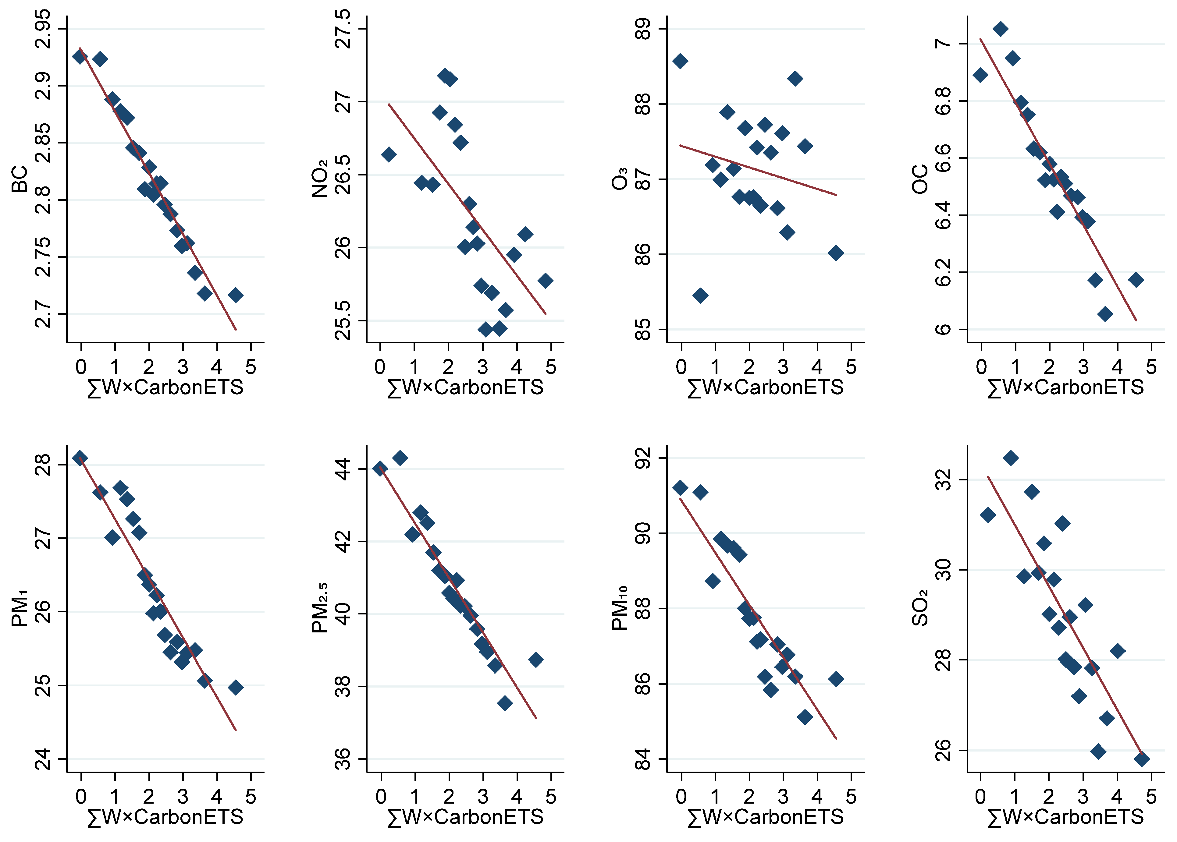
Before we proceed to a formal empirical analysis, let us first observe the preliminary visual evidence. Figure 1 is a binned scatter plot that displays the negative correlation between local atmospheric pollution levels and the “density of carbon ETS in neighboring regions”. This binned scatter plot is drawn by using data of 288 Chinese cities during 2005–2020, after controlling for region- and time-fixed effects. For a particular region i, the “density of ETS in neighboring regions” is a weighted average of the status of ETS implementation in all districts j other than region i, using the inverse of the distance between regions i and j as weights. (The detailed definition of this variable is explained in Section 2.2.) Given that the geographical distances remain constant, the value of the density will become larger when more neighboring regions implement ETS. The eight subfigures in the graph, respectively, demonstrate the circumstances of eight types of atmospheric pollutants, including black carbon (BC), nitrogen dioxide (NO2), ozone (O3), organic carbon (OC), particulate matter less than 1 micron in size (PM1), fine particulate matter (PM2.5), particulate matter less than 10 microns in size (PM10), and sulfur dioxide (SO2). From the figure, it can be observed that the degree of atmospheric pollution is lower when the density of carbon ETS in neighboring regions is greater. Based on this figure, it is reasonable to conjecture that there is a spatial spillover impact of carbon ETS that reduces air pollution in neighboring regions. To verify this conjecture, this study will utilize statistical methods for quantitative evaluation.
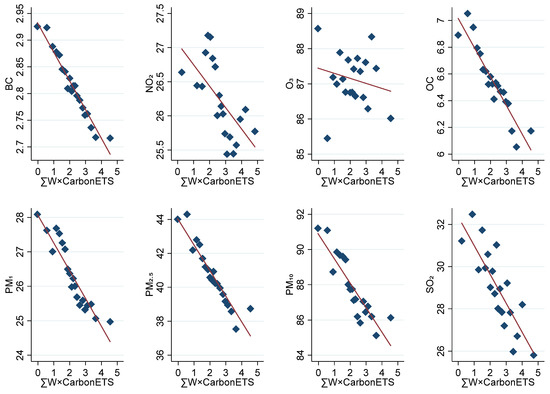
Figure 1.
The negative correlation between the density of carbon emissions trading system in neighboring regions and local air pollution. Note: (1) Air pollution is indicated by the annual average concentration of several pollutants: black carbon (BC), nitrogen dioxide (NO2), ozone (O3), organic carbon (OC), particulate matter less than 1 micron in size (PM1), fine particulate matter (PM2.5), particulate matter less than 10 microns in size (PM10), and sulfur dioxide (SO2). The measurement unit of pollution concentration is µg/m3. (2) ∑W × CarbonETS represents the density of carbon ETS in neighboring regions. It is a weighted average of the status of ETS implementation in districts other than the local region, utilizing the inverse of the distance between regions as weights. The detailed definition of this variable is explained in Section 2.2. (3) The binned scatter plot is obtained by using 20 bins. The graph would be similar if other numbers of bins are used. (4) The data sources are explained in Section 2.3.
1.2. Research Purpose, Outline, and Contributions
The research purpose of the current study is to examine whether China’s carbon ETS has spatial spillover effects on air pollution. To achieve this purpose, we employ a multiple linear regression approach to analyze panel data from 288 Chinese cities between 2005 and 2020. Unlike previous studies that focused on a limited number of air pollution indicators—particularly PM2.5 and SO2—this research examines eight air pollution metrics: BC, NO2, O3, OC, PM1, PM2.5, PM10, and SO2. To control for potential confounding factors, we follow the prior literature by incorporating a range of meteorological (e.g., precipitation, wind speed, temperature), socioeconomic (e.g., GDP per capita, population, industrial structure), and policy variables (e.g., the air pollution prevention and control action plan, low-carbon city pilot policies) as control variables in the regression models. We adopt conventional robustness testing methods, including using the one-period-lagged explanatory variable and alternative spatial weighting matrices, to verify the reliability of our empirical findings. Previous studies have extensively confirmed that environmental regulation, green innovation, energy transition, and industrial structure upgrading can effectively mitigate air pollution. Therefore, our mechanism analyses investigate whether the ETS influences these mediating variables in non-ETS regions.
The contributions of the current study lie in two aspects. (1) Whether the ETS policy has spatial spillover influences on air pollution has not been sufficiently studied in the existing research. Our study addresses this research gap. Previous studies on the spatial spillover impacts of ETS have focused on carbon leakage, i.e., the spillover effects on CO2. Our study will demonstrate that ETS generates significant beneficial impacts on air quality in non-ETS regions. This contributes to a better and deeper understanding of the environmental benefits of ETS. (2) Compared to the previous literature, this study analyzes multiple indicators of air pollution, providing a more comprehensive picture of the influences of ETS on atmospheric pollution. This offers novel empirical evidence for understanding the Chinese air pollution issues and the dynamic changes in air quality.
2. Materials and Methods
2.1. Regression Model
The current study employs the following multiple linear regression equation to estimate the spatial spillover effects of carbon ETS on air quality.
In Equation (1), the explanatory variable AirPollutionit denotes the degree of air pollution in region i in year t. The core explanatory variable in the equation is . It represents the density of carbon ETS implementation in the neighboring areas of region i. Wij is an element of a spatial weights matrix. CarbonETSjt is a binary dummy variable used to indicate whether region j executes a carbon ETS in period t or not. The covariates are grouped in two vectors, represented by ControlVariablesit and OtherPoliciesit. We will describe the meanings of these variables in detail in Section 2.2. ui, vt, and εit represent the region-fixed effect, time-fixed effect, and residual term, respectively.
The values of the regression coefficients α, β, and γ in the equation will be estimated using econometric regression methods. We employ t-tests to examine whether the regression coefficient of each individual explanatory variable is statistically significant. All analyses are conducted using Stata 15 statistical software, which computes the t-statistics and their corresponding p-values automatically. We report the t-statistic values in our results. To assess the overall significance of the regression models, we perform F-tests to determine whether all explanatory variables jointly exert statistically significant influences on the dependent variables. Since all regression models in this study pass the F-test, we omit reporting the specific F-statistic values to conserve space in the article.
The coefficient of interest in this study is α, which captures the aggregate impact of ETS implemented in all other regions j ≠ i on the air pollution in local region i. A significantly negative value of coefficient α means that ETS generates a beneficial spatial spillover impact on air quality. In this case, the ETS implemented in region j decreases air pollution in region i by |α × Wij|. In contrast, a significantly positive value of coefficient α indicates that ETS has an adverse spatial spillover effect on air quality. In this case, the ETS implemented in region j increases air pollution in region i by |α × Wij|.
It is notable that, the coefficient α also captures the impact of ETS implemented in local region i on air pollution in other regions j ≠ i. A significant value of coefficient α indicates that the ETS implemented in region i would cause air pollution in region j to change by α × Wji.
2.2. Variables
2.2.1. Dependent Variables
The explained variable in the current study is AirPollutionit, the level of air pollution. Air pollution is caused by multiple kinds of pollutants. In this study, we inspect the spillover impacts of carbon ETS on each of the eight air pollutants: BC, NO2, O3, OC, PM1, PM2.5, PM10, and SO2, respectively. The unit of pollution concentration is µg/m3.
2.2.2. Core Explanatory Variable of Interest
The core explanatory variable of interest in this study is . It represents the density of carbon ETS implementation in the neighboring areas of region i. This variable is a weighted average of the status of ETS implementation in all districts j other than region i, with the inverse of the distance between regions i and j as weights. Wij is an element in a spatial weights matrix commonly used in the spatial econometrics literature, defined as follows:
In Equation (2), Distanceij is the geographic distance (in units of 100 km) between region i and region j. We calculate the distance between two cities on the basis of the latitude and longitude coordinates of the center of each city. CarbonETSjt is a binary dummy variable used to indicate whether region j implements a carbon ETS in period t or not.
The assumption behind Equation (2) is that the implementation of the ETS in region j may have an impact on region i, and this impact is inversely proportional to the distance between regions i and j. After summing up the impacts of all other regions j ≠ i on the local region i, which is expressed by , we measure the aggregate impact of the ETS implemented in all other regions on the local region.
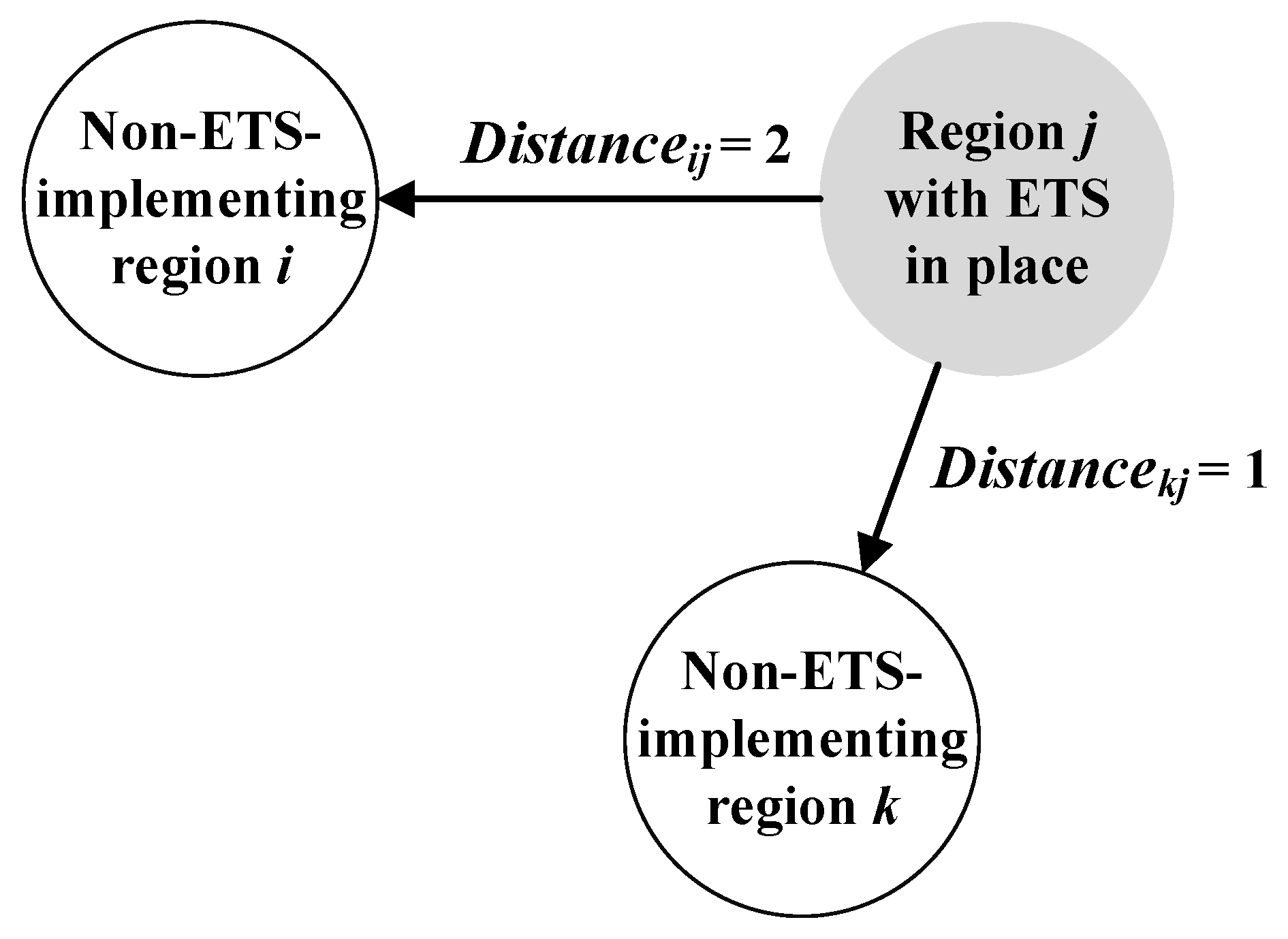
To more clearly explain the spatial spillover impacts of ETS on other regions that the current study aims to measure, we use Figure 2 for illustration. Suppose there are three regions, i, j, and k, where region j has implemented ETS while regions i and k have not. We assume the distance between regions i and j is Distanceij = 2, and the distance between regions k and j is Distancekj = 1. The ETS implemented in region j generates spillover effects, influencing air pollution levels in regions i and k. For region i, the spillover effect from region j is ; for region k, the spillover effect from region j is .

Figure 2.
Illustration of the spatial spillover impacts of ETS on other regions.
2.2.3. Covariates
Following the previous literature, we use a set of covariates to control for potential confounding factors. Covariates are included in two groups: ControlVariablesit and OtherPoliciesit. ControlVariablesit contains twelve meteorological and socioeconomic factors: precipitation (Precipitationit), sunlight duration (Sunlightit), wind speed (WindSpeedit), temperature (Temperatureit), GDP per capita (GDPPerCapitait), population density (PopulationDensityit), share of tertiary industry in the economy (TertiaryIndustryit), financial development (FinancialDevelopmentit), trade openness (TradeOpennessit), high-speed railway (HighSpeedRailwayit), road density (RoadDensityit), and medical infrastructure (MedicalInfrastructureit). OtherPoliciesit contains thirty binary dummy variables representing some place-based public policies relevant to environmental and economic issues. To save space, we put the detailed explanations on these covariates in Appendix A.
2.3. Data Source and Sample
The data were from several sources. (1) The data source of BC, OC, and PM1 pollution data was NASA’s MERRA-2 M2T1NXAER product. The data source of NO2, O3, and PM10 was the GlobalHighAirPollutants (GHAP) dataset [24,25,26]. The data source of PM2.5 was the Satellite-derived PM2.5 V6.GL.02.02 dataset [27]. The data source of SO2 was The Reports on the State of the Environment of China written by China’s Ministry of Ecology and Environment. The original data provided by these data sources were processed to calculate the annual average values of various pollutants for each Chinese city. With the exception of SO2 data, which were initially provided by official Chinese ground monitoring stations, all other air pollutant data are derived from remote sensing datasets processed in previous studies. The specific technical details can be found in the relevant literature. (2) The data source of meteorological variables was the ERA5-Land dataset of the European Union’s Copernicus Climate Change Service. (3) The source of high-speed railway data was the CNRDS (Chinese Research Data Services Platform). (4) The information about different public policies was manually collected from relevant governmental websites. (5) The other variables such as GDP per capita and population were downloaded from the EPS China Data.
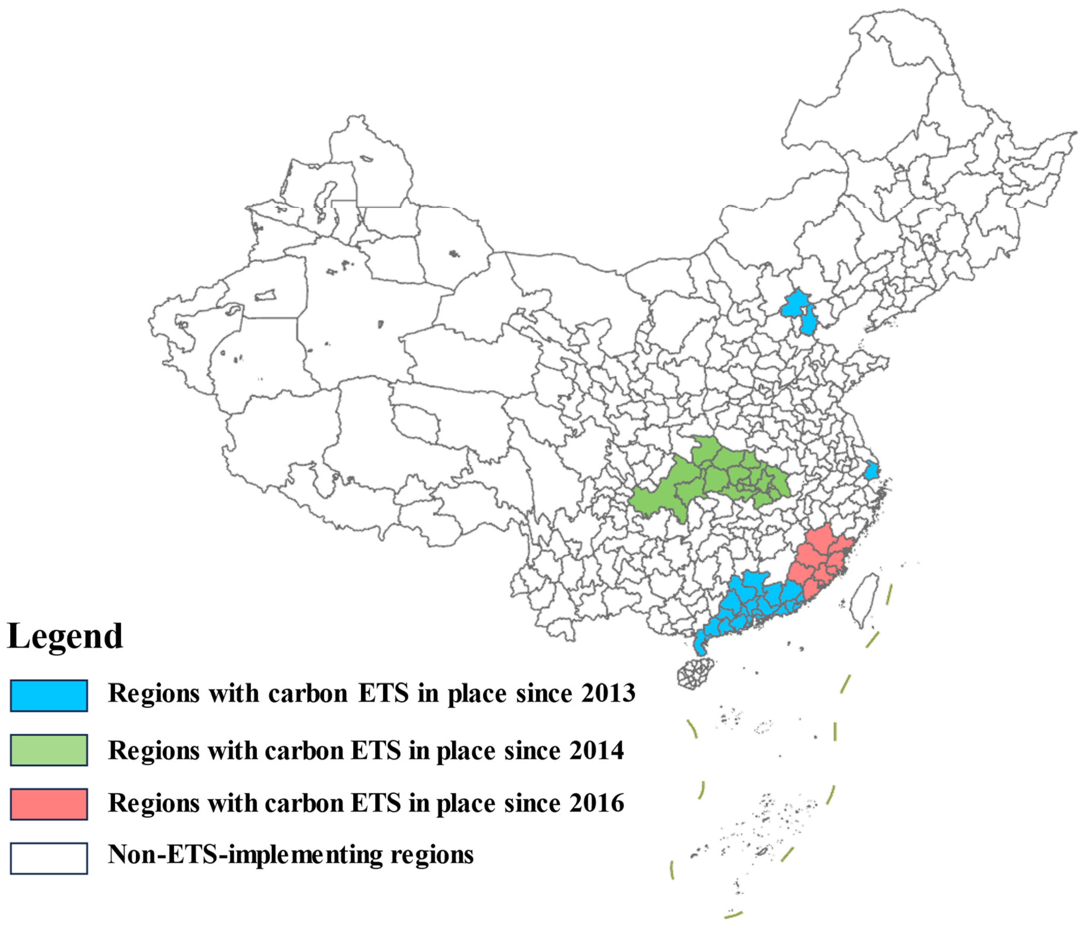
Our analysis is on the basis of the data for 288 Chinese cities between 2005 and 2020. The data are at annual frequency. In order to focus on analyzing the spatial spillover impacts of carbon ETS, we excluded from our study sample cities that have implemented the ETS policy locally, which are located within seven province-level administrative units (Beijing, Chongqing, Fujian, Guangdong, Hubei, Shanghai, and Tianjin). In the sample period, all the sample cities did not implement carbon ETS locally and, thus, the impacts of ETS on these cities were from spatial spillovers. China has over 330 prefecture-level and province-level cities in total. After excluding all ETS-implementing cities and those with missing data, we finally retained 288 non-ETS cities for the empirical analysis. China’s cap-and-trade carbon ETS pilot project was rolled out in three batches, implemented in 2013, 2014, and 2016, respectively. Our research sample covers 8 years before the policy (from 2005 to 2012) and 8 years after the policy (from 2013 to 2020). Since China began to implement a nationwide carbon ETS policy in 2021, which affected all regions, our analysis does not include data after 2021. Figure 3 shows the geographical distribution of cities with and without ETS implementation. We did not perform special treatment for missing values. If a variable had missing data for a certain city-year observation, that particular data point was simply dropped. Consequently, our data are unbalanced panel data. Table 1 reports the descriptive statistics of main variables.

Figure 3.
Geographical distribution of cities with and without ETS implementation.

Table 1.
Descriptive statistics of main variables.
2.4. Methods of Robustness Tests
In order to ensure that the regression results based on Equation (1) are robust, we conduct three robustness checks. First, we consider that there may be a time lag in the policy effect of the ETS. Therefore, in the first robustness test, we use the one-year-lagged explanatory variable, , for the regression analysis. We also consider that the regression results are dependent on the spatial weights matrix we choose. Therefore, in the second and third robustness tests, we use alternative spatial weights matrices: W0.5 and W2. The elements in these two matrices are defined as follows:
2.5. Methods of Mechanism Analyses
To explore how the spillover effects of carbon ETS occur, we examine four possible mechanisms. Existing studies have confirmed that environmental regulation, green innovation, low-carbon energy transition, and industrial structure upgrading can effectively mitigate atmospheric pollution. If ETS promotes these mechanism variables in non-ETS regions, air pollution in non-ETS regions is likely to decrease. In the mechanism analyses, we replace the dependent variable in Equation (1) with these mechanism variables to estimate the effects of . Statistically significant coefficients indicate that the tested mechanisms hold, thereby providing explanations for the spatial spillover influences of the carbon ETS.
3. Results
3.1. Main Results
Table 2 provides the coefficient estimates for Equation (1). When the explained variables are BC, NO2, OC, PM1, PM2.5, and PM10, the estimated coefficients of ∑W × CarbonETS are all negative and statistically significant at the 1% level. This indicates that when the density of ETS policies in neighboring areas increases, the pollution concentrations of BC, NO2, OC, PM1, PM2.5, and PM10 in local area would decrease. When the explained variables are O3 and SO2, the estimated coefficients of ∑W × CarbonETS are not statistically significant, although the coefficients are also negative. This suggests that local O3 and SO2 pollution levels are not significantly affected by ETS policies in other regions. Overall, the results provided in Table 2 indicate that carbon ETS generates a significant spatial spillover effect on air pollution. The execution of carbon ETS improves air quality in non-ETS regions.
Table 2.
Estimated spillover effects of carbon ETS on air pollution.
The coefficients of some covariates in Table 2 are also statistically significant. This implies that air pollution is also affected by the covariates. Since we focus on the spillover influences of ETS in this study, we do not discuss the coefficients of the covariates in detail.
Based on our empirical findings, we can reasonably draw the following two inferences. (1) Starting from 2013, as the ETS pilot policy was implemented in certain regions and generated beneficial spatial spillover effects, the concentrations of BC, NO2, OC, PM1, PM2.5, and PM10 in non-ETS regions also experienced a significant decline. (2) The higher the “density of carbon ETS in neighboring regions” (i.e., ∑W × CarbonETS), the greater the reduction in air pollutant concentrations.
These inferences align with the actual trends in China’s air pollution. We illustrate this point using a figure. Based on whether a city’s average “density of carbon ETS in neighboring regions” (i.e., ∑W × CarbonETS) during the sample period was above the sample median, we divide the sample cities in this study into two groups: the group of large ∑W × CarbonETS and the group of small ∑W × CarbonETS. Figure 4 presents the trends in BC, NO2, OC, PM1, PM2.5, and PM10 for these two groups from 2005 to 2020. Before 2013, air pollution levels in both groups remained relatively stable or even increased slightly. However, starting in 2013, both groups exhibited a significant decline in atmospheric pollution, with the group of large ∑W × CarbonETS showing a more pronounced decrease in pollutant concentrations. The patterns displayed in Figure 4 explicitly support the empirical results reported in Table 2: the ETS policy has generated significant spatial spillover effects, leading to reduced air pollution in non-ETS regions.
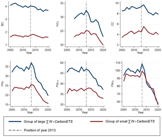
Figure 4.
Changes in various air pollutants in the sample cities between 2005 and 2020. Note: (1) The measurement unit of pollution concentration is µg/m3. (2) ∑W × CarbonETS represents the density of carbon ETS in neighboring regions. It is a weighted average of the status of ETS implementation in districts other than the local region, using the inverse of the distance between regions as weights. (3) The NO2 data between 2005 and 2007 are not displayed due to data unavailability.
3.2. Robustness Tests
In order to ensure that the previous regression results are robust, we conduct three robustness checks. In the first robustness test, we use the one-year-lagged explanatory variable, , for the regression analysis. In the second and third robustness tests, we use alternative spatial weights matrices: W0.5 and W2.
The results of these three robustness tests are provided in Panels A, B, and C of Table 3. These results are well consistent with the previous results reported in Table 2. We detect that ETS has a beneficial spatial spillover impact on air quality. The ETS significantly reduces the local BC, NO2, OC, PM1, PM2.5, and PM10 pollution in non-ETS regions.
Table 3.
Coefficient estimates for robustness tests.
3.3. Heterogeneity Tests
In previous analyses, we treated all cities in the sample as homogeneous units and evaluated the “average” spillover effects of carbon ETS on all cities. However, it is possible that the spillover effects vary by city characteristics. For instance, highly industrialized regions and cities with high population density may be more sensitive to environmental policies, leading to stronger ETS spillover effects in these areas. We now conduct heterogeneity tests to assess whether the spillover impacts of ETS differ across regions.
We employ the following empirical strategy. We select a specific city characteristic and divide the sample cities into two groups: Group 1 and Group 2. We then construct two binary dummy variables, DiGroup1 and DiGroup2, to indicate which group city i belongs to. If city i is in Group 1, then DiGroup1 = 1 and DiGroup2 = 0; if it belongs to Group 2, then DiGroup1 = 0 and DiGroup2 = 1. We multiply these two dummy variables by to obtain two interaction terms: and . We then replace in Equation (1) with these two interaction terms to derive Equation (5). The coefficients and in Equation (5) measure the spatial spillover impacts of carbon ETS on cities in Group 1 and Group 2, respectively.
We conducted five types of grouping based on the city’s industrialization level, population density, economic development level, resource endowment, and geographical location. (1) Based on the average share of secondary industry in GDP during the sample period, we classified cities into the group with high industrialization level and the group with low industrialization level. The heterogeneity test results are presented in Panel A of Table 4. (2) Based on population density, we divided cities into the group with high population density and the group with low population density. The regression results are shown in Panel B. (3) Using per capita GDP, we categorized cities into the group with high economic development level and the group with low economic development level. The results are reported in Panel C. (4) Following the official list from the “National Sustainable Development Plan for Resource-Based Cities (2013–2020)” published by China’s central government in 2013, we separated cities into the group of resource-based cities and the group of non-resource-based cities. The results appear in Panel D. (5) By geographic location, we distinguished between the group of cities in eastern region and the group of cities in central and western regions. Panel E displays the regression results.
Table 4.
Coefficient estimates for heterogeneity tests.
As shown in Panels A–E of Table 4, the coefficients for both interaction terms— and —are mostly significantly negative across different city groups, except in a few cases where they are statistically nonsignificant. In other words, the beneficial spatial spillover effects of ETS on air quality can be observed across different groups of cities. Moreover, it is important to note that the regression coefficients are generally similar among different groups. Therefore, we actually did not detect significant heterogeneity. These results also indicate that the core findings of this study are highly robust.
3.4. Mechanism Analyses
In previous analyses, we have already detected that carbon ETS has significant spatial spillover impacts, reducing air pollution in other regions. Next, we explore how the effects occur. We examine four possible mechanisms: environmental regulation, green innovation, low-carbon energy transition, and industrial structure upgrading. If ETS promotes environmental regulation, green innovation, energy transition, and industrial upgrading in other regions, air pollution in other regions is likely to decrease. Below, we analyze, respectively, whether the ETS changes these four variables in neighboring regions.
First, we inspect the spillover influence of carbon ETS on the degree of environmental regulation. We need to construct an environmental regulation indicator. Following the previous literature [28,29], we measure the stringency of environmental regulation within a city by the proportion of environment-related words in the text of the local government’s annual work reports. The higher value of this indicator represents that the local government pays more attention to ecological protection and the environmental regulation is stricter. We replace the dependent variable in Equation (1) with this environmental regulation indicator and estimate the impact of ∑W × CarbonETS. As indicated by the coefficient reported in column (i) of Table 5, we do not find a significant impact of ETS on the environmental regulation stringency in other regions.
Table 5.
Coefficient estimates for mechanism analyses.
Second, we analyze the spillover effects of ETS on green innovation. To measure green innovation, we add 1 to the number of green patent applications in a city during one corresponding year and then take the logarithm. The data of green patent applications were available in the CNRDS database. We estimate the impact of ∑W × CarbonETS using green innovation as the explained variable. The estimated coefficient of ∑W × CarbonETS is provided in column (ii) of Table 5. The coefficient is significantly positive, indicating that ETS significantly encourages green innovation in the neighboring areas.
Third, we analyze the low-carbon energy transition. We choose the low-carbon energy transition index constructed by Shen et al. [30] to measure a city’s performance toward low-carbon energy transition. The larger value of this index represents better performance on the energy transition path. We use this index to replace the dependent variables in Equation (1). The regression results displayed in column (iii) of Table 5 suggest that ∑W × CarbonETS significantly promotes low-carbon energy transition.
Fourth, we investigate the industrial structure upgrading. Referring to the previous literature [31,32,33], we utilize an index (ISU) to track the progress of industrial structure upgrading. ISU = I1 + I2 × 2 + I3 × 3 where I1, I2, and I3 represent the proportion of value added of the primary industry, secondary industry, and tertiary industry in GDP, respectively. The larger the value of ISU, the higher the degree of industrial structure upgrading. We use ISU as the explained variable. The regression result displayed in column (iv) of Table 5 shows that ∑W × CarbonETS substantially contributes to industrial structure upgrading.
To further analyze the temporal dynamics of mechanism effects, we adopt the following model to estimate the influence of the ETS across different years:
Here, Yit represents the mechanism variables under study, including environmental regulation, green innovation, low-carbon energy transition, and industrial structure upgrading. I(t = k) is an indicator function that equals 1 if t = k, and equals 0 otherwise. For example, when k = 2013, if the observation is from the year of 2013 (i.e., t = 2013), then I(t = k) = 1; otherwise, I(t = k) = 0. The coefficient αk captures the spatial spillover impact of the carbon ETS in year k. Using Equation (6), we are able to estimate the spillover impacts of the carbon ETS on the mechanism variables in each year from 2013 to 2020.
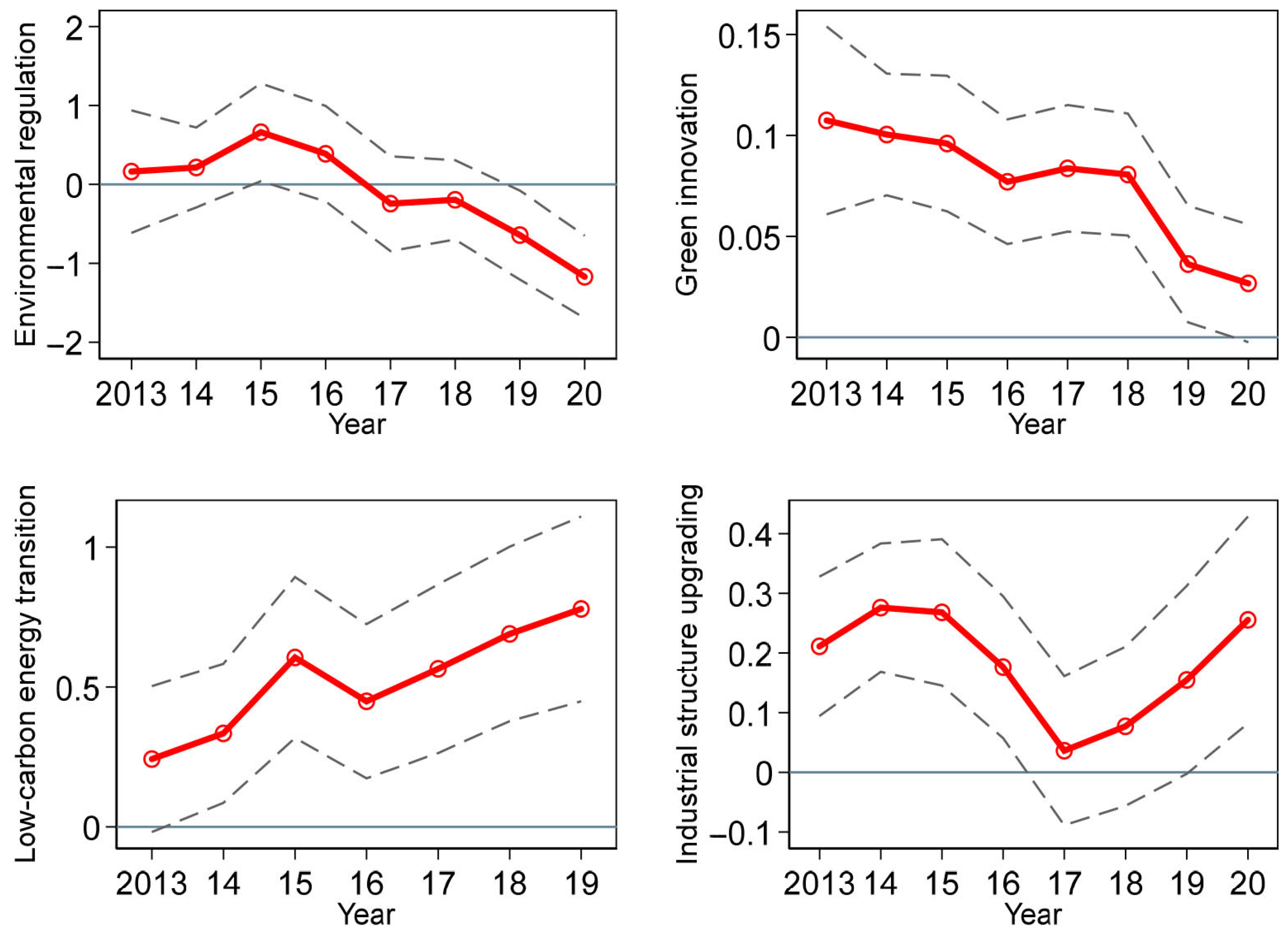
To visualize the dynamic effects of the ETS on these mechanism variables, we present the regression results in Figure 5. The four subplots depict the annual impacts of the ETS on environmental regulation, green innovation, low-carbon energy transition, and industrial structure upgrading, corresponding to the estimated coefficients αk for each year. The graph reveals several key findings. (1) The spillover effects of ETS on environmental regulation are generally statistically nonsignificant. (2) The spillover effect on green innovation exhibits temporal decay: the effect peaked in 2013 and gradually diminished over time. (3) The effect on low-carbon energy transition demonstrates temporal strengthening: the effect started from the smallest magnitude in 2013 and progressively increased in subsequent years. (4) The impact on industrial structure upgrading shows fluctuation dynamics: the impact reached its maximum in 2014, declined to a trough in 2017, then rebounded in subsequent years to form an approximate U-shaped pattern.
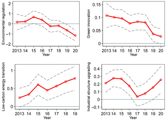
Figure 5.
The dynamic spillover effects of carbon ETS on environmental regulation, green innovation, low-carbon energy transition, and industry structure upgrading. Note: (1) In the figure, the circles on the red lines represent the point estimates of the coefficients αk in Equation (6), while the gray dashed lines indicate the 90% confidence intervals. (2) Due to data unavailability, the figure does not display the impact on low-carbon energy transition in 2020.
In short, the mechanism analyses indicate that carbon ETS promotes green innovation, low-carbon energy transition, and industrial structure upgrading in non-ETS regions. The magnitude of ETS’s effects on these mechanism variables exhibits distinct temporal patterns across years. While its spillover effect on green innovation demonstrates a diminishing trend over time, the impact on low-carbon energy transition shows progressive strengthening, and the influence on industrial structure upgrading displays cyclical fluctuations.
4. Discussion
This study reveals that the implementation of the carbon ETS can significantly reduce air pollution concentrations in non-ETS regions, thereby improving air quality. We conducted a series of robustness tests, experimenting with different model specifications with alternative temporal windows and spatial neighborhood definitions. We also performed heterogeneity tests, considering various ways to group sample cities. These tests consistently support our core findings regarding the beneficial spatial spillover influences of the ETS.
Although the effects estimated in this study are indirect effects arising through spatial spillovers, the magnitude of these indirect effects is of practical significance. Based on our coefficient estimates and the variable values in the sample, we can calculate the marginal effects of the ETS on specific pollutants. For example, let us consider the scenario in 2020. In our sample, in 2020, the mean value of the implementation density of ETS, i.e., ∑W × CarbonETS, was 4.895. On average, if the number of cities implementing the ETS were to double (assuming these cities are uniformly and randomly distributed across China’s territory), this would double ∑W × CarbonETS, increasing its mean value by 4.895. This would lead to an additional reduction in air pollutant concentrations in a typical non-ETS city by |α × Δ(∑W × CarbonETS)|, where α is the coefficient value reported in Table 2 and Δ(∑W × CarbonETS) is the change in the implementation density of ETS. For instance, the concentration of BC would decrease by 0.0384 × 4.895 = 0.188 µg/m3. Similarly, we can calculate that the concentrations of NO2, OC, PM1, PM2.5, and PM10 would decrease by 0.822, 0.871, 3.099, 5.737, and 6.848 µg/m3, respectively. These environmental benefits carry substantial public health and economic gains. The findings of the current study have valuable academic and practical implications, which we elaborate on below.
4.1. Academic Implications
From the perspective of academic research, first, the findings in this study demonstrate that, when evaluating the impacts of ETS, its spatial spillover effect on the environment cannot be overlooked. The previous literature primarily used the DID method to ex-post evaluate the pros and cons of ETS. A core assumption of the traditional DID method is the absence of spatial spillover effects [14,15]. Our study reveals that the spatial spillover effects of ETS on air quality are significant and ETS can improve air quality in other regions. Therefore, conclusions drawn from past studies using the traditional DID method may be biased. Ignoring the beneficial spatial spillover influences of ETS on air quality would lead to an underestimation of its benefits.
Second, our study uncovers a crucial co-benefit: reducing greenhouse gas emissions often brings additional benefits in reducing other air pollutants, because they share common emission sources. This finding is consistent with some prior studies. For instance, Basaglia et al. [34] estimated that the EU ETS significantly reduced toxic air pollutants, such as SO2, PM2.5, and NOx, and these pollution reductions would translate into substantial health gains, potentially amounting to hundreds of billions of Euros. Similarly, Zhang et al. [35] found that cooperative international efforts to reduce greenhouse gases could bring substantial air quality co-benefits to the United States. Therefore, beyond greenhouse gas reduction, ETS has significant environmental co-benefits, which should be fully recognized when evaluating the benefits of ETS.
4.2. Practical Implications
First, this study emphasizes the existence of spatial spillover effects from ETS. This suggests that implementing ETS may play a crucial role in countries with serious atmospheric pollution problems, such as China, India, and Pakistan. Since ETS generates positive externalities, governments should support enterprises across regions to actively participate in carbon emissions trading. Our findings indicate that the environmental benefits of ETS extend beyond administrative boundaries, significantly improving air quality in other areas by reducing BC, NO2, OC, PM1, PM2.5, and PM10. However, these benefits diminish with increasing geographic distance. Thus, the development of carbon trading markets should persistently advance regional integration of policies [6,36,37]. Governments should strongly promote regionally coordinated carbon markets or gradually expanding ETS coverage on various economic sectors, to encourage firms across regions to take advantage of the carbon market, to leverage these spatial synergistic effects. When more regions participate in ETS, greater collective benefits can be achieved [38,39], thereby maximizing the spatial effectiveness of carbon markets design and environmental policies. It is worth noting that due to these positive externalities, some regions may have incentives to free ride by benefiting from others’ efforts without reducing their own emissions. Therefore, when designing carbon markets and various environmental policies, governments should pay attention to their potential spatial spillover effects and address possible free-riding problems through cooperation and coordination mechanisms among regions, such as cross-regional consultation, benefit compensation mechanisms, and regional joint emission reduction agreements.
Second, we also emphasize that China’s ETS should not be viewed as an isolated climate policy tool, but rather as part of an integrated climate–air quality policy portfolio. In practice, ETS can work alongside other environmental policies in China such as the “Blue Sky Defense War”, regional carbon neutrality plans, and the “Air Pollution Prevention and Control Action Plan”, to jointly achieve the dual goals of mitigating climate change and improving air quality.
Finally, our study scores the need to integrate ETS into the government’s long-term environmental protection strategy system to maximize its co-benefits. First, the government should promote technological innovation and low-carbon energy transition as key complementary policies to carbon ETS. Local governments can leverage the national carbon market platform to accelerate the cultivation of green industries, improve the green financial system, and foster a virtuous cycle of green development. Second, ETS can serve as a crucial policy tool for implementing the long-term strategy of “Beautiful China 2035”, supporting China’s transition towards a sustainable, low-carbon future. “Beautiful China 2035” emphasizes not only to reduce greenhouse gas emissions and improve air quality, but also to seek comprehensive improvements across various ecological aspects such as water quality, land, and forests [40]. Since carbon ETS can promote green innovation, low-carbon energy transition, and industrial structure upgrading, it has the potential to generate benefits for other aspects of the ecosystem.
5. Conclusions and Limitations
5.1. Conclusions
This study investigates the spatial spillover impacts of carbon ETS on air pollution in areas where the policy is not implemented. By analyzing data for 288 Chinese cities from 2005 to 2020, this study finds that the carbon ETS policy significantly reduces BC, NO2, OC, PM1, PM2.5, and PM10 concentrations in non-ETS regions. This result suggests that the beneficial effects of the ETS on air quality exist not only in the ETS-implementing areas, as already noted by the previous literature, but also extend to the areas where ETS is not implemented. The heterogeneity tests reveal consistent evidence of the ETS’s beneficial spatial spillover effects, which remain statistically significant across cities characterized by different levels of industrialization, population density, economic development, resource endowments, and geographical locations. Further mechanism analyses show that although the policy does not significantly change the level of environmental regulation in other regions, it promotes green innovation, low-carbon energy transition, and industrial structure upgrading in neighboring regions. These phenomena provide plausible explanations for the observed spatial spillover effects of policy.
5.2. Limitations and Future Research Directions
Our study contains several limitations that point to valuable avenues for future research.
- (1)
- Since our analysis relies on Chinese data, it remains unclear whether the conclusions regarding the spillover effects of ETS could be generalizable to other countries. Future studies could apply our methodology to examine the ETS programs in other countries, such as the EU ETS, US ETS, or Canadian ETS, to investigate whether similar spatial spillovers exist.
- (2)
- Our data coverage ended in 2020, precluding analysis of post-2021 developments. This cutoff was necessary because China launched its national carbon market in 2021, resulting in universal ETS coverage across all cities. There were no non-ETS cities after 2021. Consequently, our regression model (which captures the impact of ETS on non-ETS cities) became inapplicable. Future researchers could employ more sophisticated models coupled with granular data on policy intensity or trading volumes to analyze the national market’s effects after 2021.
- (3)
- This study focuses exclusively on the spillovers of carbon ETS without accounting for potential spillovers from other policies. China has implemented numerous environmental and regional development policies. Certain policies may also generate spatial spillover effects on air pollution. Future research could examine other critical policies, such as the Air Pollution Prevention and Control Action Plan, the Low-carbon City Pilot Project, and the Three-year Action Plan to Fight Air Pollution, to investigate their potential cross-regional spillover effects.
Author Contributions
Conceptualization, D.D.; methodology, D.D.; validation, D.D.; data curation, D.Z. and D.D.; formal analysis, D.Z. and D.D.; software, D.Z. and D.D.; visualization, D.Z. and D.D.; writing—original draft, D.Z. and D.D.; writing—review and editing, D.Z. and D.D. All authors have read and agreed to the published version of the manuscript.
Funding
This research received no external funding.
Institutional Review Board Statement
Not applicable.
Informed Consent Statement
Not applicable.
Data Availability Statement
The data are available from the corresponding author upon request.
Conflicts of Interest
The authors declare no conflicts of interest.
Appendix A
Table A1 provides a list of covariates included in “ControlVaraiblesit”. Table A2 provides a list of policies included in “OtherPoliciesit”.
Table A1.
List of covariates included in “ControlVariables”.
Table A1.
List of covariates included in “ControlVariables”.
| Covariates in “ControlVariables” | Definitions |
|---|---|
| Precipitation | Precipitation, the logarithmic value of annual precipitation level (mm) |
| Sunlight | Sunlight duration, the logarithmic value of annual sunlight duration (h) |
| WindSpeed | Wind speed, the logarithmic value of annual average wind speed (m/s) |
| Temperature | Temperature, the annual average temperature (°C) |
| GDPPerCapita | GDP per capita, the logarithmic value of GDP per capita (RMB) measured in the price level in 2020 |
| PopulationDensity | Population density, the logarithmic value of population density (person/km2), i.e., the number of residents per unit of land |
| TertiaryIndustry | Share of tertiary industry, the value added in tertiary industry as a proportion of local GDP |
| FinancialDevelopment | Financial development level, the ratio of bank credits to local GDP |
| TradeOpenness | Trade openness level, the ratio of international trade size to local GDP |
| HighSpeedRailway | High-speed railway, dummy variable for the high-speed railway, equals 1 if the city is connected to the nationwide high-speed railway network, and equals 0 otherwise |
| RoadDensity | Road density, the logarithmic value of road density, the ratio of road length (km) to land area (km2) |
| MedicalInfrastructure | Abundance of public medical infrastructure, the logarithmic value of the number of hospital beds per thousand residents |
Table A2.
List of policies included in “OtherPolicies”.
Table A2.
List of policies included in “OtherPolicies”.
| Names of Policies | Definitions of Corresponding Dummy Variables |
|---|---|
| Air pollution prevention and control action plan | Set binary dummy variables Dit for each policy, which equals 1 if the corresponding policy was implemented in region i in year t, and equals 0 otherwise |
| Broadband China pilot project | |
| Circular-economy city pilot project | |
| Clean energy demonstration provinces | |
| Clean winter-heating plan in Northern China | |
| Comprehensive demonstration cities for energy saving and emission reduction fiscal policies | |
| Cross-border e-commerce comprehensive pilot zones | |
| Demonstration zones for industrial transformation and upgrading in old industrial cities and resource-based cities | |
| Ecological environment monitoring pilot zones | |
| E-commerce demonstration cities project | |
| Energy-use rights trading system pilot zones | |
| Grassland ecological compensation policy | |
| Household registration system reform | |
| Information benefiting-the-people pilot cities | |
| Internet demonstration cities | |
| Low-carbon city pilot project | |
| National big data comprehensive pilot zones | |
| National ecological conservation pilot zones | |
| National independent innovation demonstration zones | |
| National new-type urbanization comprehensive pilot zones | |
| National sustainable development plan for resource-based cities | |
| New energy demonstration cities | |
| Pilot project to promote the integration of technology and finance | |
| Plan on the rise in Central China | |
| Pollution emissions trading system pilot zones | |
| Resource-exhausted city support policy | |
| Smart-city pilot project | |
| Smart-tourism city pilot project | |
| South-to-north water diversion project | |
| Three-year action plan to fight air pollution |
References
- Almond, D.; Zhang, S. Carbon-trading pilot programs in China and local air quality. AEA Pap. Proc. 2021, 111, 391–395. [Google Scholar] [CrossRef]
- Shi, X.; Xu, Y.; Sun, W. Evaluating China’s pilot carbon Emission Trading Scheme: Collaborative reduction of carbon and air pollutants. Environ. Sci. Pollut. Res. 2024, 31, 10086–10105. [Google Scholar] [CrossRef]
- Dong, Z.; Xia, C.; Fang, K.; Zhang, W. Effect of the carbon emissions trading policy on the co-benefits of carbon emissions reduction and air pollution control. Energy Policy 2022, 165, 112998. [Google Scholar] [CrossRef]
- Li, C.; Jin, H.; Tan, Y. Synergistic effects of a carbon emissions trading scheme on carbon emissions and air pollution: The case of China. Integr. Environ. Assess. Manag. 2024, 20, 1112–1124. [Google Scholar] [CrossRef]
- Liu, J.-Y.; Woodward, R.T.; Zhang, Y.-J. Has carbon emissions trading reduced PM2.5 in China? Environ. Sci. Technol. 2021, 55, 6631–6643. [Google Scholar] [CrossRef]
- Dai, S.; Qian, Y.; He, W.; Wang, C.; Shi, T. The spatial spillover effect of China’s carbon emissions trading policy on industrial carbon intensity: Evidence from a spatial difference-in-difference method. Struct. Change Econ. Dyn. 2022, 63, 139–149. [Google Scholar] [CrossRef]
- Li, S.; Liu, J.; Wu, J.; Hu, X. Spatial spillover effect of carbon emission trading policy on carbon emission reduction: Empirical data from transport industry in China. J. Clean. Prod. 2022, 371, 133529. [Google Scholar] [CrossRef]
- Li, Z.; Wang, J. Spatial emission reduction effects of China’s carbon emissions trading: Quasi-natural experiments and policy spillovers. Chin. J. Popul. Resour. Environ. 2021, 19, 246–255. [Google Scholar] [CrossRef]
- Cui, J.; Wang, C.; Zhang, J.; Zheng, Y. The effectiveness of China’s regional carbon market pilots in reducing firm emissions. Proc. Natl. Acad. Sci. USA 2021, 118, e2109912118. [Google Scholar] [CrossRef]
- Qin, W.; Xie, Y. The impact of China’s emission trading scheme policy on enterprise green technological innovation quality: Evidence from eight high-carbon emission industries. Environ. Sci. Pollut. Res. 2023, 30, 103877–103897. [Google Scholar] [CrossRef]
- Wen, H.; Chen, Z.; Nie, P. Environmental and economic performance of China’s ETS pilots: New evidence from an expanded synthetic control method. Energy Rep. 2021, 7, 2999–3010. [Google Scholar] [CrossRef]
- Wu, Q. Price and scale effects of China’s carbon emission trading system pilots on emission reduction. J. Environ. Manag. 2022, 314, 115054. [Google Scholar] [CrossRef] [PubMed]
- Yan, Y.; Zhang, X.; Zhang, J.; Li, K. Emissions trading system (ETS) implementation and its collaborative governance effects on air pollution: The China story. Energy Policy 2020, 138, 111282. [Google Scholar] [CrossRef]
- Berg, T.; Reisinger, M.; Streitz, D. Spillover effects in empirical corporate finance. J. Financ. Econ. 2021, 142, 1109–1127. [Google Scholar] [CrossRef]
- Delgado, M.S.; Florax, R.J.G.M. Difference-in-differences techniques for spatial data: Local autocorrelation and spatial interaction. Econ. Lett. 2015, 137, 123–126. [Google Scholar] [CrossRef]
- Jiang, X.; Li, G.; Fu, W. Government environmental governance, structural adjustment and air quality: A quasi-natural experiment based on the Three-year Action Plan to Win the Blue Sky Defense War. J. Environ. Manag. 2021, 277, 111470. [Google Scholar] [CrossRef]
- Cui, L.; Zhou, J.; Peng, X.; Ruan, S.; Zhang, Y. Analyses of air pollution control measures and co-benefits in the heavily air-polluted Jinan city of China, 2013–2017. Sci. Rep. 2020, 10, 5423. [Google Scholar] [CrossRef]
- Li, W.; Shao, L.; Wang, W.; Li, H.; Wang, X.; Li, Y.; Li, W.; Jones, T.; Zhang, D. Air quality improvement in response to intensified control strategies in Beijing during 2013–2019. Sci. Total Environ. 2020, 744, 140776. [Google Scholar] [CrossRef]
- Yang, X.; Teng, F. The air quality co-benefit of coal control strategy in China. Resour. Conserv. Recycl. 2018, 129, 373–382. [Google Scholar] [CrossRef]
- Greenstone, M.; Hanna, R. Environmental regulations, air and water pollution, and infant mortality in India. Am. Econ. Rev. 2014, 104, 3038–3072. [Google Scholar] [CrossRef]
- Majumdar, D.; Purohit, P.; Bhanarkar, A.D.; Rao, P.S.; Rafaj, P.; Amann, M.; Sander, R.; Pakrashi, A.; Srivastava, A. Managing future air quality in megacities: Emission inventory and scenario analysis for the Kolkata Metropolitan City, India. Atmos. Environ. 2020, 222, 117135. [Google Scholar] [CrossRef]
- Shahbazi, H.; Hassani, A.; Hosseini, V. Evaluation of Tehran clean air action plan using emission inventory approach. Urban Clim. 2019, 27, 446–456. [Google Scholar] [CrossRef]
- Lupo, M.; Sofia, D.; Barletta, D.; Poletto, M. Calibration of DEM simulation of cohesive particles. Chem. Eng. Trans. 2019, 74, 379–384. [Google Scholar] [CrossRef]
- Wei, J.; Li, Z.; Xue, W.; Sun, L.; Fan, T.; Liu, L.; Su, T.; Cribb, M. The ChinaHighPM10 dataset: Generation, validation, and spatiotemporal variations from 2015 to 2019 across China. Environ. Int. 2021, 146, 106290. [Google Scholar] [CrossRef] [PubMed]
- Wei, J.; Li, Z.; Li, K.; Dickerson, R.; Pinker, R.; Wang, J.; Liu, X.; Sun, L.; Xue, W.; Cribb, M. Full-coverage mapping and spatiotemporal variations of ground-level ozone (O3) pollution from 2013 to 2020 across China. Remote Sens. Environ. 2022, 270, 112775. [Google Scholar] [CrossRef]
- Wei, J.; Li, Z.; Wang, J.; Li, C.; Gupta, P.; Cribb, M. Ground-level gaseous pollutants (NO2, SO2, and CO) in China: Daily seamless mapping and spatiotemporal variations. Atmos. Chem. Phys. 2023, 23, 1511–1532. [Google Scholar] [CrossRef]
- Shen, S.; Li, C.; van Donkelaar, A.; Jacobs, N.; Wang, C.; Martin, R.V. Enhancing global estimation of fine particulate matter concentrations by including geophysical a priori information in deep learning. ACS EST Air 2024, 1, 332–345. [Google Scholar] [CrossRef]
- Chen, Z.; Kahn, M.E.; Liu, Y.; Wang, Z. The consequences of spatially differentiated water pollution regulation in China. J. Environ. Econ. Manag. 2018, 88, 468–485. [Google Scholar] [CrossRef]
- Zhang, J.; Chen, S. Financial development. environmental regulations and green economic transition. J. Financ. Econ. 2021, 47, 78–93. (In Chinese) [Google Scholar] [CrossRef]
- Shen, Y.; Shi, X.; Zhao, Z.; Xu, J.; Sun, Y.; Liao, Z.; Li, Y.; Shan, Y. A dataset of low-carbon energy transition index for Chinese cities 2003–2019. Sci. Data 2023, 10, 906. [Google Scholar] [CrossRef]
- Ren, X.; Zeng, G.; Gozgor, G. How does digital finance affect industrial structure upgrading? Evidence from Chinese prefecture-level cities. J. Environ. Manag. 2023, 330, 117125. [Google Scholar] [CrossRef] [PubMed]
- Wu, L.; Sun, L.; Qi, P.; Ren, X.; Sun, X. Energy endowment, industrial structure upgrading, and CO2 emissions in China: Revisiting resource curse in the context of carbon emissions. Resour. Policy 2021, 74, 102329. [Google Scholar] [CrossRef]
- Xu, L.; Shu, H.; Lu, X.; Li, T. Regional technological innovation and industrial upgrading in China: An analysis using interprovincial panel data from 2008 to 2020. Financ. Res. Lett. 2024, 66, 105621. [Google Scholar] [CrossRef]
- Basaglia, P.; Grunau, J.; Drupp, M.A. The European Union Emissions Trading System might yield large co-benefits from pollution reduction. Proc. Natl. Acad. Sci. USA 2024, 121, e2319908121. [Google Scholar] [CrossRef]
- Zhang, Y.; Bowden, J.H.; Adelman, Z.; Naik, V.; Horowitz, L.W.; Smith, S.J.; West, J.J. Co-benefits of global and regional greenhouse gas mitigation for US air quality in 2050. Atmos. Chem. Phys. 2016, 16, 9533–9548. [Google Scholar] [CrossRef]
- Li, Z.; Wang, J. Spatial spillover effect of carbon emission trading on carbon emission reduction: Empirical data from pilot regions in China. Energy 2022, 251, 123906. [Google Scholar] [CrossRef]
- Yang, Z.; Yuan, Y.; Zhang, Q. Carbon emission trading scheme, carbon emissions reduction and spatial spillover effects: Quasi-experimental evidence from China. Front. Environ. Sci. 2022, 9, 824298. [Google Scholar] [CrossRef]
- Mandaroux, R.; Schindelhauer, K.; Mama, H.B. How to reinforce the effectiveness of the EU emissions trading system in stimulating low-carbon technological change? Taking stock and future directions. Energy Policy 2023, 181, 113697. [Google Scholar] [CrossRef]
- Zeng, Y.; Faure, M.G.; Feng, S. Localization vs globalization of carbon emissions trading system (ETS) rules: How will China’s national ETS rules evolve? Clim. Policy 2025, 1–15. [Google Scholar] [CrossRef]
- Ma, Z.; Cui, H.; Ge, Q. Future climatic risks faced by the Beautiful China Initiative: A perspective for 2035 and 2050. Adv. Clim. Change Res. 2025, 16, 141–153. [Google Scholar] [CrossRef]

Disclaimer/Publisher’s Note: The statements, opinions and data contained in all publications are solely those of the individual author(s) and contributor(s) and not of MDPI and/or the editor(s). MDPI and/or the editor(s) disclaim responsibility for any injury to people or property resulting from any ideas, methods, instructions or products referred to in the content. |
© 2025 by the authors. Licensee MDPI, Basel, Switzerland. This article is an open access article distributed under the terms and conditions of the Creative Commons Attribution (CC BY) license (https://creativecommons.org/licenses/by/4.0/).