The Analysis of the Extreme Cold in North America Linked to the Western Hemisphere Circulation Pattern

Abstract

The Western Hemisphere (WH) circulation pattern was discovered in recent years through Self-Organizing Maps (SOMs) clustering of the Northern Hemisphere 500 hPa geopotential height during winter. For example, the extremely cold wave that occurred in North America during 2013–14 is associated with WH circulation anomalies. We discussed the extremely cold weather conditions within the WH pattern during the winter season from 1979 to 2023. The variations of cold air in North America during the WH pattern have been demonstrated using the NCEP/NCAR reanalysis datasets. By defining WH events and North American extremely cold events, we have identified a connection between the two. In extremely cold events, linear winds are the key factor driving the temperature drop, as determined by calculating temperature advection. The ridge in the Gulf of Alaska serves as an early signal for this cold weather. The WH circulation anomaly triggers an anomalous ridge in the Gulf of Alaska region, leading to trough anomalies downstream over North America. This results in the southward movement of cold air from the polar regions, causing cooling in the mid-to-northern parts of North America. With the maintenance of the stationary wave in the North Pacific (NP), the anomalous trough over North America can be deepened, driving cold air into the continent. Influenced by the low pressure over Greenland and the storm track, the cold anomalies are concentrated in the central and northern parts of North America. This cold air situation persists for approximately two weeks. The high-level patterns of the WH pattern in both the 500 hPa height and the troposphere level have been identified using SOM. This cold weather is primarily a tropospheric phenomenon with limited correlation to stratospheric activities.

1. Introduction

Extremely cold weather has always been a noteworthy weather phenomenon, and previous works [1,2] have analyzed the sources and destinations of cold air in the Northern Hemisphere. There have been numerous studies that prove the correlation between teleconnection patterns and extreme weather [3,4,5,6,7,8]. A distinct negative phase of the North Atlantic Oscillation (NAO) is observed a week before cold air outbreaks in the United States [9,10,11], and the Pacific-North America (PNA) pattern is also crucial for predicting mid-latitude cold air. The cold weather in North America is also affected by the stratospheric polar vortex [12,13]. Anticyclones in northern Alaska and cyclones in the Labrador Sea can push Arctic cold air southward, while the airflow behind the Alaska High often intensifies the anomalously low-pressure trough in the North of the United States, allowing the cold pool to move southward. On the intra-seasonal timescale, the Arctic Oscillation (AO) and the Northern Annular Mode (NAM) are closely associated with extremely cold weather in North America [14,15].

Previous studies [16] have shown that an extremely cold weather event occurred in the United States during the winter of 2013–2014, which was related to the enhancement of the North Pacific Oscillation (NPO)/Western Pacific (WP). A further study [17] indicated that the extremely cold weather in 2013–2014 was caused by a significant deviation from normal circulation patterns. Specifically, the cold air jet stream over the Arctic was split into two parts, located over North America and Siberia. In fact, the circulation anomaly that dominated the 2013–2014 winter was referred to as the Western Hemisphere (WH) pattern [18], which resembles a Rossby wave train propagating from the North Pacific to North America.

Bao et al. [19] utilized the Self-Organizing Map (SOM) to categorize the winter circulation patterns from 1979 to 2014 into various types, with the second mode being the WH circulation pattern (as shown in Figure 1). Tan et al. [20] found that although the spatial structure of the WH circulation pattern is similar to that of PNA and NAO in some regions, it is not a simple superposition of PNA and NAO but a newly discovered low-frequency variability in the atmosphere independent of NAO and PNA, which is the third monthly EOF mode (NAO and PNA are the first and second modes, respectively). Previous works have explored the main physical mechanism of the formation and maintenance of the WH pattern [18,20]. The results show that the propagation of steady Rossby waves, the eddy feedback process [18] and the energy conversion process related to the background field [20] all contribute to the maintenance of the WH pattern.

Although previous works have interpreted the formation and maintenance mechanisms of the WH pattern, the specific impact of the WH pattern on the Northern Hemisphere climate variability is still unrevealed. Considering the extreme cold in North America during the 2013–2014 winter, which is associated with evident WH anomalies, it is implied that the WH pattern is associated with the extremely cold event in North America. This article will focus on the positive phase of WH and describe in detail what impact WH will have on North America. Section 2 presents the data and methods. Section 3 explains the process of temperature changes within ECEs and the key contributions that influence temperature variations. Section 4 is the 500 hPa result of SOM. The summary is provided in Section 5.

2. Data and Methods

2.1. Datas and Extremely Cold Events

In this study, the datasets used are based on the NCEP/NCAR (National Centers for Environmental Prediction/National Center for Atmospheric Research) reanalysis [21] on a 2.5° × 2.5° grid, spanning from 1979 to 2023. The datasets are available on 17 pressure levels from 1000 to 10 hPa. The daily mean geopotential height, 2 m temperature, zonal winds, longwave radiation, shortwave radiation, latent heat flux, and sensible heat flux were analyzed for the period from December 1979 to April 2023.

Fourty-four persistent winter datasets were created by combining the above reanalysis data. Anomalies are obtained by removing the seasonal cycle averaged over 1979–2023. To identify persistent patterns, this study employs a 10-day low-pass filter to remove fluctuations with periods shorter than 10 days, thereby retaining long-term climate signals. The daily time series of the Western Hemisphere Index (WHI) was obtained by calculating the spatial regression coefficients of the 10-day low-pass-filtered 500 hPa geopotential height anomalies poleward of 20° N on the WH pattern (Figure 1). The daily values of the coefficients were normalized using the standard deviation of the entire time series to obtain the WHI [18]. The WH events with 12 consecutive days of WHI greater than 0.7 as the emergence of WH circulation were identified. After completing the statistics of WH events, the composite results indicate that the primary region of extreme temperatures is located in North America. Figure 2 shows the low-temperature region used in this study for the statistical analysis following the composite of WH events. Here, we used the region of 45° N~65° N, 50° W~115° W to study the extremely cold weather conditions in North America. The average temperature of this region was regarded as the Cold Air Index (CI),

$$\mathrm{C}\mathrm{o}\mathrm{l}\mathrm{d} \mathrm{a}\mathrm{i}\mathrm{r} \mathrm{i}\mathrm{n}\mathrm{d}\mathrm{e}\mathrm{x} = {\mathrm{T}}_{\mathrm{N}\mathrm{A}}$$

(1)

${\mathrm{T}}_{\mathrm{N}\mathrm{A}}$ denotes the regional average temperature of the region mentioned above (Figure 2). Extremely cold weather will be considered to occur when the ${\mathrm{T}}_{\mathrm{N}\mathrm{A}}$ is below 252 K, which means lower than 90% of winter days. The process of maintaining extremely cold weather for 4 days or more is considered a persistent extremely cold event (ECE); each event maintains an interval of 7 days or more. We obtained 40 persistent extremely cold events from the surface level. It should be pointed out that the data detrending calculation does not affect the final result. Figure 3 shows the distribution of ECEs. Previous research [22] has recorded a super cold weather in North America in the winter of 1983–1984. The study pointed out that the blocking system in the Gulf of Alaska caused the outbreak of this super-low temperature weather, which corresponds to the characteristics of WH anomalies and ECEs defined in this study.

2.2. The Temperature Advection Methods

The thermodynamic equation implemented in the reanalysis model can be written as follows:

$${\displaystyle \frac{\partial T}{\partial t}}=-u{\displaystyle \frac{\partial T}{\partial x}}-v{\displaystyle \frac{\partial T}{\partial y}}-\dot{\eta }{\displaystyle \frac{\partial T}{\partial \eta }}+{\displaystyle \frac{kT\omega }{p}}+P_T+Res$$

(2)

According to the equation, we can state that the factors that can change the temperature are divided into horizontal temperature advection $-u{\displaystyle \frac{\partial T}{\partial x}}-v{\displaystyle \frac{\partial T}{\partial y}}$, vertical temperature advection $-\dot{\eta }{\displaystyle \frac{\partial T}{\partial \eta }}$, adiabatic warming ${\displaystyle \frac{kT\omega }{p}}$, and non-adiabatic heating $P_T$. Based on previous research summaries, the most significant factor in changing temperature is the horizontal temperature advection term. We adopted the temperature contribution algorithm by Clark and Feldstein [23]:

$$-\mathbf{u}·\nabla \mathrm{T}=-{\mathbf{u}}^{\prime }·\nabla \overline{\mathrm{T}}-\overline{\mathbf{u}}·\nabla {\mathrm{T}}^{\prime }-{\mathbf{u}}^{\prime }·\nabla {\mathrm{T}}^{\prime }-\overline{\mathbf{u}}·\nabla \overline{\mathrm{T}},$$

(3)

where overbars denote a smoothed daily climatology, and primes denote deviation. Therefore, u = (u, v, 0), $\nabla \equiv$ ($\partial /\partial \mathrm{x}$, $\partial /\partial \mathrm{y}$, 0). Removing the smoothed seasonal cycle from the advection terms yields, the expression for the advection anomaly is the following:

$$\begin{gathered} -\mathit{u}·\nabla T+\overline{\mathit{u}·\nabla T} \\ =(-\mathit{u}’·\overline{\nabla T}+\overline{\mathit{u}’·\overline{\nabla T}}) \\ +(-\overline{\mathit{u}}·\nabla T’+\overline{\overline{\mathit{u}}·\nabla T’}) \\ +(-\mathit{u}’·\nabla T’+\overline{\mathit{u}’·\nabla T’}) \\ +\left(-\overline{\mathit{u}}·\overline{\nabla T}+\overline{\overline{\mathit{u}}·\overline{\nabla T}}\right) \end{gathered}$$

(4)

The equation states that the horizontal temperature advection anomaly is driven by the anomalous advection of the climatological temperature by the anomalous wind $-\mathbf{u}’·\nabla \overline{\mathrm{T}}+\overline{\mathbf{u}’·\nabla \overline{\mathrm{T}}}$ (linear wind), the anomalous advection of the anomalous temperature by the climatological wind $-\overline{\mathbf{u}}·\nabla \mathrm{T}’+\overline{\overline{\mathbf{u}}·\nabla \mathrm{T}’}$ (linear temperature), the anomalous advection of the anomalous temperature by the anomalous wind $-\mathbf{u}’·\nabla \mathrm{T}’+\overline{\mathbf{u}’·\nabla \mathrm{T}’}$ (nonlinear), and an additional term reflecting the small difference between $-\overline{\mathbf{u}}·\nabla \overline{\mathrm{T}}$ and $\overline{-\overline{\mathbf{u}}·\nabla \overline{\mathrm{T}}}$. In the following sections, the first term is called the linear wind term, the second term is the linear temperature term, the third term is the nonlinear term, and the last is the mean term.

2.3. The Cold Air Mass and Flux Methods

The cold air mass (CAM) index with the isentropic cold air mass analysis [24,25] is used to research the role of cold air. According to Iwasaki et al. [25], using the governing equation for the geographical distribution of cold air masses, the CAM amount (DP) is the vertical depth of the atmosphere below a designated potential temperature θ_T and is calculated as follows:

$$\mathrm{D}\mathrm{P}={\mathrm{p}}_{\mathrm{s}}-\mathrm{p}\left({\mathsf{\theta }}_{\mathrm{T}}\right),$$

(5)

where ${\mathrm{p}}_{\mathrm{s}}$ is the ground surface pressure, and p(${\mathsf{\theta }}_{\mathrm{T}}$) is the pressure on isentrope θ = θ_T. According to previous studies [25,26], we set θ_T = 280 K. The CAM flux is given by the following:

$$\mathrm{F}={\int }_{\mathrm{p}\left({\mathsf{\theta }}_{\mathrm{T}}\right)}^{{\mathrm{p}}_{\mathrm{s}}}\mathit{u}\mathrm{d}\mathrm{p},$$

(6)

where u is the horizontal wind vector. We used the Negative Heat Content (NHC) to measure the cold air mass [25,27]; the NHC can be considered as an indicator to denote the lower troposphere’s change and also can define the strength of “cold wave”. The NHC is generated by diabatic cooling at all levels below θ_T and affected by the surface diabatic heating:

$$\mathrm{N}\mathrm{H}\mathrm{C}={\int }_{{\mathrm{p}}_{\left({\mathsf{\theta }}_{\mathrm{T}}\right)}}^{{\mathrm{p}}_{\mathrm{s}}}\left({\mathsf{\theta }}_{\mathrm{T}}-\mathsf{\theta }\right)dp,$$

(7)

2.4. Diagnosis of Vertical Propagation of Planetary Waves

On the other hand, we want to discuss whether there is a connection between the stratosphere and the troposphere during the WH circulation. To diagnose the impact of the stratosphere, the eddy meridional heat flux (V*·T*) is used as a signal to evaluate the vertical propagation of Rossby waves between the stratosphere and troposphere. Here, the asterisk indicates the zonal deviation. The intensity of the polar vortex in the stratosphere will affect the outbreak or blockage of cold air in the mid-latitude troposphere [12,13,28]. We found that the results of the stratosphere can also explain the characteristics of ECEs to some extent. Kodera [29] identified the form of troughs and ridges in the troposphere can be altered to some extent by the strength of planetary wave reflection or the intensity of downward propagation from the stratosphere. Therefore, we referenced the reflection index (RI) and downwelling index (DI) of the stratosphere:

$$\mathrm{D}\mathrm{I}={\left(V^{*}·T^{*}\right)}_{NA},$$

(8)

$$\mathrm{R}\mathrm{I}={(V^{*}·T^{*})}_{AL}-{(V^{*}·T^{*})}_{NA},$$

(9)

where subscript NA denotes the region-averaged eddy meridional heat flux of North America (60° N~85° N, 80° W~130° W), and subscript AL denotes the region-averaged flux of Alaska (50° N~75° N, 150° E~160° W). Figure 4 shows the eddy heat flux and the selected region.

2.5. Self-Organizing Maps

In order to better distinguish the characteristics of WH, we used the Self-Organizing Maps (SOMs) clustering method. This method is a two-dimensional array of maps that display characteristic patterns [30,31,32]. Based on the theoretical study by Bao and Wallace [19], the circulation patterns obtained through SOM clustering have no significant differences from those derived from EOFs. In order to discuss the diversity of ECEs within the WH circulation patterns. By using SOM clustering, we distinguished different groups among the 40 ECEs, ranging from a 1 × 3 matrix to a 1 × 8 matrix in the diagnostic process. During this process, it can be found that there is no significant difference between even-numbered matrices such as 2 × 4 and the 1 × 8 result. Therefore, this study only uses the $1·\mathrm{n}$computational approach for clustering, where n represents the number of categories. Through this method, ECEs can be categorized into four circulation patterns with distinct characteristics.

2.6. Surface Energy Budget

Some variations in surface temperature can be explained through radiative flux, following Clark and Feldstein [23], Gong et al. [33] and Lee et al. [34], and the discussion of SAT, G can be written as follows:

$$\mathrm{G}={\int }_0^{{\mathsf{\delta }}_{\mathrm{z}}}\mathsf{\rho }{\mathrm{c}}_{\mathrm{p}}\left({\displaystyle \frac{\mathrm{d}\mathrm{T}}{\mathrm{d}\mathrm{t}}}\right)\mathrm{d}\mathrm{z}$$

(10)

G denotes energy storage at the surface. Then, G can also be written as follows:

$$\mathrm{G}={\mathrm{F}}_{\mathrm{l}\mathrm{w}}^{\downarrow }+{\mathrm{F}}_{\mathrm{l}\mathrm{w}}^{\uparrow }{+\mathrm{F}}_{\mathrm{s}\mathrm{w}}^{\downarrow }+{\mathrm{F}}_{\mathrm{s}\mathrm{w}}^{\uparrow }+{\mathrm{F}}_{\mathrm{s}\mathrm{h}}+{\mathrm{F}}_{\mathrm{l}\mathrm{h}}+\mathrm{R},$$

(11)

where F_lw and F_sw denote longwave and shortwave radiation, F_sh and F_lh denote sensible heat flux and latent heat flux, and the superscripts $\uparrow$ and $\downarrow$ denote the upward and downward direction. R denotes the term that can cause changes in surface temperature due to other factors (such as sea ice variations). The following differential is considered:

$$∆\mathrm{G}={∆\mathrm{F}}_{\mathrm{l}\mathrm{w}}^{\downarrow }+∆{\mathrm{F}}_{\mathrm{l}\mathrm{w}}^{\uparrow }{+∆\mathrm{F}}_{\mathrm{s}\mathrm{w}}^{\downarrow }+{∆\mathrm{F}}_{\mathrm{s}\mathrm{w}}^{\uparrow }+{∆\mathrm{F}}_{\mathrm{s}\mathrm{h}}+{∆\mathrm{F}}_{\mathrm{l}\mathrm{h}}+∆\mathrm{R},$$

(12)

where the operator $∆$ denotes the anomaly. G can be taken to represent the energy storage within an infinitesimally thin interface at the surface, the G = 0 [33,34]. According to Joseph [23], by subtracting $∆$G from both sides of Equation (11), a new residual term can be calculated as $∆\mathrm{R}-∆$G:

$$∆\mathrm{R}-∆\mathrm{G}=-∆{\mathrm{F}}_{\mathrm{l}\mathrm{w}}^{\downarrow }-∆{\mathrm{F}}_{\mathrm{l}\mathrm{w}}^{\uparrow }-{∆\mathrm{F}}_{\mathrm{s}\mathrm{w}}^{\downarrow }-{∆\mathrm{F}}_{\mathrm{s}\mathrm{w}}^{\uparrow }-{∆\mathrm{F}}_{\mathrm{s}\mathrm{h}}-{∆\mathrm{F}}_{\mathrm{l}\mathrm{h}}$$

(13)

The residual over land, therefore, reflects only the physical process contained in $∆\mathrm{R}$. The longwave radiation, shortwave radiation, sensible heat flux, and latent heat flux here are all normalized by the quantity $4\mathsf{\sigma }{\mathsf{\epsilon }}_{\mathrm{s}}{\left\{{\mathrm{T}}_{\mathrm{s}}\right\}}^3$ in order to better compare the relationship between radiations and temperature.

3. Result

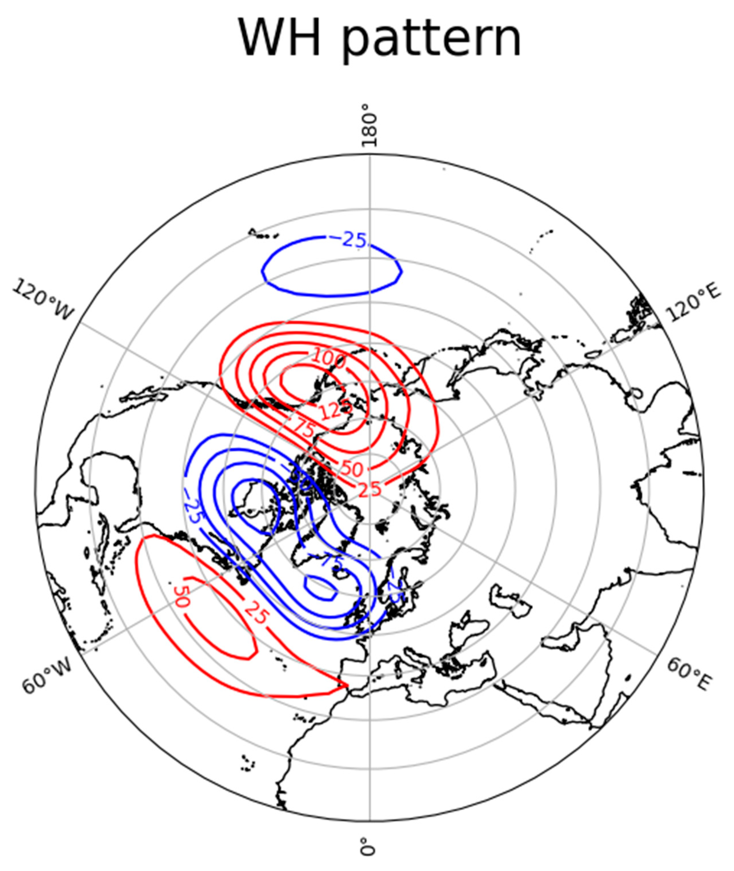
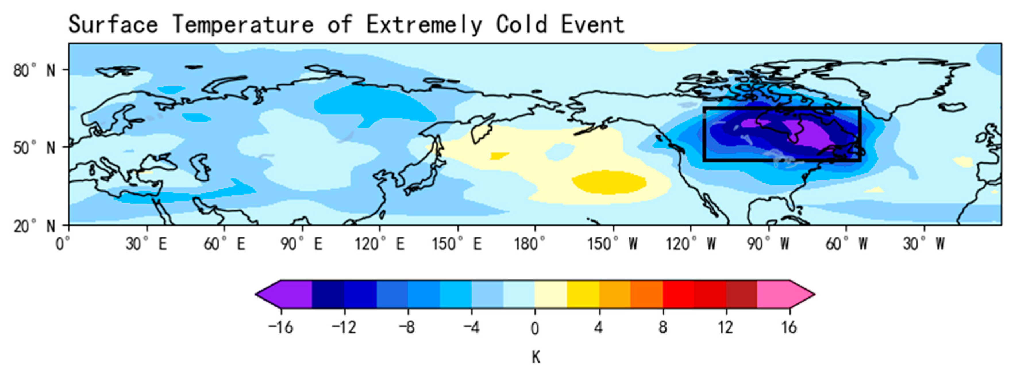
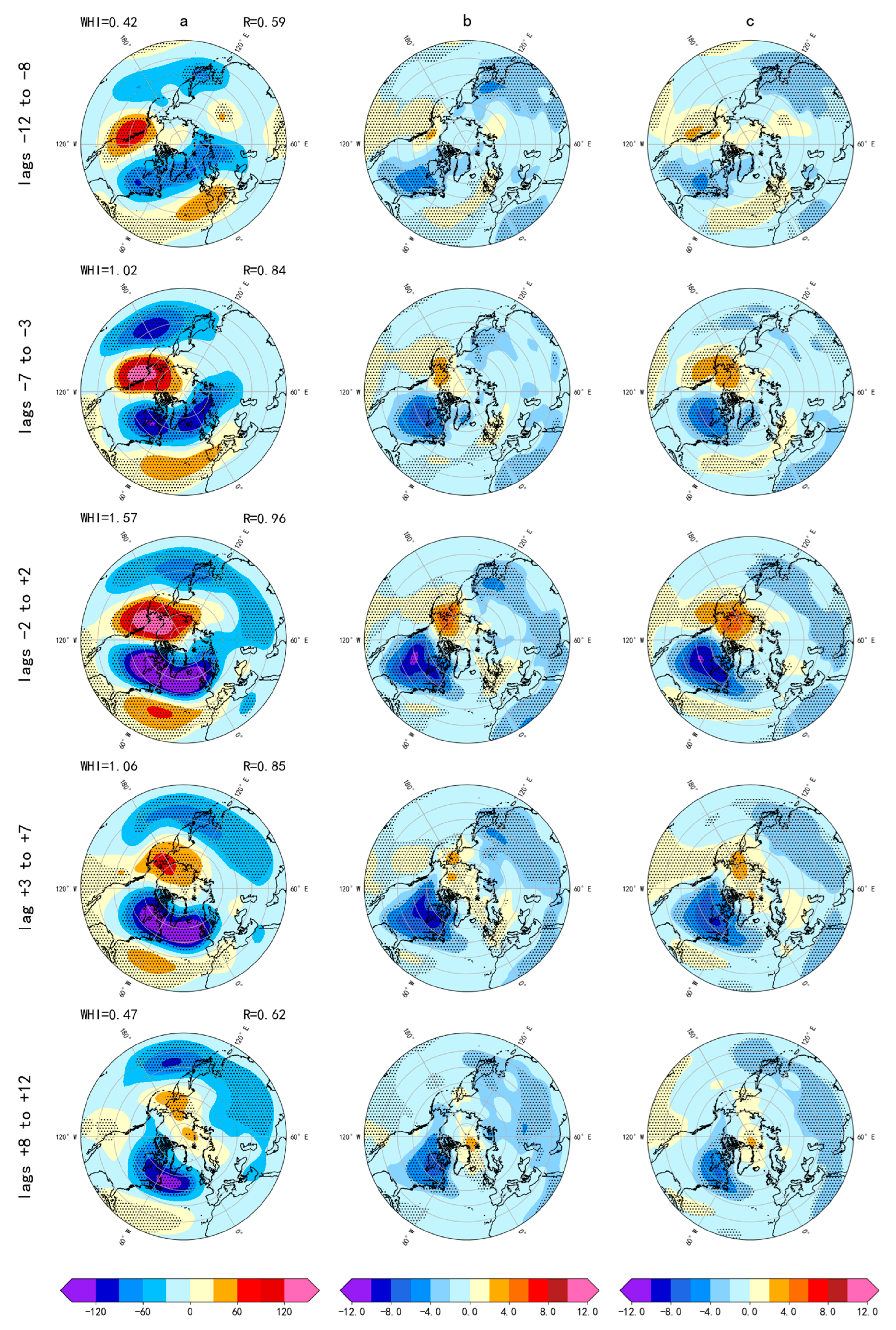
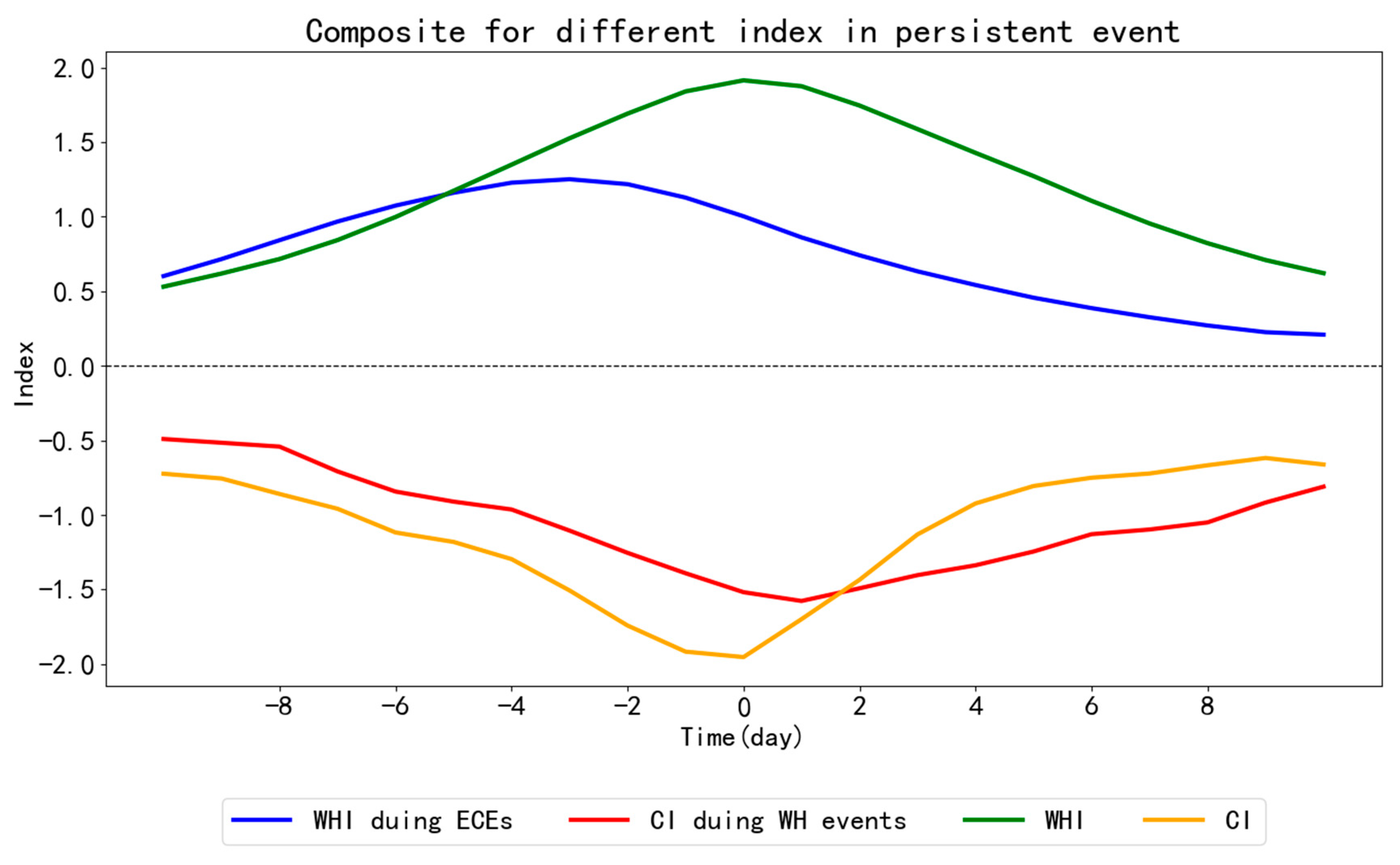
3.1. The Developments of WH and ECEs in North America

As shown in Figure 1, the WH circulation pattern is characterized by positive geopotential height anomalies over Alaska and negative geopotential height anomalies over North America. After applying the regression results of WH to the winters from 1979 to 2023 and defining WH events, we obtained a composite map of events featuring the WH circulation pattern during these winters (Figure 5). By setting day 0 as the day with the highest WHI of the WH pattern and setting the time scale to cover the 12 days before and after day 0, it can be observed that the WH circulation can persist for approximately two weeks. The main temperature and geopotential height positive signal are revealed in the Alaska region (Figure 5a), while the main negative signal is revealed in North America (Figure 5a). This negative signal extends across the North Atlantic to Europe. Since the appearance of the WH day −8 signal in the Atlantic, the intensity of the dipole between the northern and central Atlantic shows a positive correlation to some extent, which may be the result of the north–south distribution of air masses of different properties caused by the storm tracks. The surface temperature and temperature at 850 hPa, which are shown in Figure 5b,c, confirmed that North America is the main region affected by extremely cold weather. It can be intuitively inferred from the figure that the WH circulation pattern can cause temperature drops in the mid-to-high latitudes of North America; the cold air outbreaks in North America are associated with anomalies in the 500 hPa geopotential height. Although the WH circulation pattern can persist for more than 2 weeks, the actual duration during which it can cause temperature drops on the North American continent is more than 1 week; there was a significant temperature drop in the mid-high latitudes of North America (40° N to 80° N), with the average temperature falling by 6 °C (Figure 6b). As can be shown in Figure 5b, temperature drops began to occur from day −7, and the North American continent remained in an abnormally low-temperature environment until day +7. The cooling regions near the ground were more concentrated in the continent (Figure 5b), while the cooling areas in the troposphere at 500 hPa and upper level spread eastward to the Atlantic Ocean, with an average temperature drop of about 3 °C (Figure 5c). Therefore, the WH circulation pattern can cause severe temperature drops in North America and even the Atlantic region.

According to the method mentioned in Section 2, the days when with the highest cold index are day 0 through the ECEs; after statistically analyzing the average temperature within the black boxed area in Figure 2, we obtained the ECE pattern in the WH circulation. Then, we obtained these 40 events, treating them in the same manner as we did with the temporal dimension of WH. The ECEs’ pattern is divided into five stages according to the method mentioned above. Figure 6 shows the ECEs’ anomalous 500 hPa geopotential height, anomalous 500 hPa temperature and 500 hPa temperature variation. The results from the 500 hPa geopotential height clearly show a good coupling relationship with the statistically derived 500 hPa temperature of ECEs, indicating that the WH circulation pattern does lead to temperature drops in the North American continent. It can be seen (Figure 6b) that the temperature in the North American continent began to drop from day −5. By day 0, the average temperature in the mid-to-high latitudes of the North American continent had dropped by 10 °C, and the cooling situation weakened after maintaining for about 3 days. In the early stage (Figure 6a), an abnormal trough appeared in the Gulf of Alaska, which gradually intensified from day −7 to day −4. With the transmission of the stationary wave, the downstream trough became stable and moved towards the Atlantic Ocean, and the entire upper air of North America was affected by the deep, cold, low pressure. Later, this cold low pressure moved to the Atlantic Ocean and reached Europe in the higher troposphere; the cold high pressure in the lower troposphere also reached the middle of the Atlantic Ocean. Thus, there is a significant barotropic component in the extremely cold weather of the WH pattern. By comparing the geopotential height of ECEs (Figure 6a) with the results of WH events (Figure 5a), it is evident that when ECEs occur, the troposphere exhibits a strong WH circulation anomaly signal. From the temperature variation (Figure 6c), it can be observed that the North American region experiences the most significant temperature changes from day −5 to day +5. There is a noticeable cooling area on the western side of the Atlantic, indicating that the cold air in ECEs also moves from Newfoundland to the ocean. This is likely related to the storm tracks that occur in North America, as information on geopotential height reveals a clear north-south symmetrical high-low center in the mid-to-high latitudes of the Atlantic region.

Figure 7 is the same as Figure 6 but at 850 hPa. The information in Figure 6 provides a better explanation for the cooling effect of ECEs. By comparing Figure 6 with Figure 7, it is evident that the closer to the surface level, the larger the area of cooling and the greater the magnitude of temperature decrease. Unlike the geopotential height at 500 hPa, the positive geopotential height anomaly in the Alaska region at 850 hPa is stronger (Figure 6a and Figure 7a). This makes it easier for cold air from the Arctic to descend into downstream areas, allowing for the observation of large-scale temperature drops as early as day −5 at 850 hPa (Figure 7b), with an average temperature decrease of 6 °C. By day 0, some regions even experienced a temperature drop of 15 °C (Figure 7b). The geopotential height on day −5 in both Figure 5 and Figure 6 collectively reflect that in ECEs, it is the intensification of positive geopotential height anomalies in Alaska that leads to the enhancement of negative geopotential height anomalies in downstream North America on day 0. The difference lies in that temperatures closer to the ground level are more susceptible to this forcing, resulting in the rapid occurrence and development of extremely cold weather. The consistency in the information of temperature variation fields also confirms that the region most affected by ECEs remains North America, with the only difference being that the temperature recovery process occurs faster at lower levels than at higher levels. This study also conducted an analysis of the association between WH events and ECEs, with the results shown in Figure 8. In the early stages of WH events, the CI index reaches peak values, indicating that WH circulation anomalies lead to significant cooling in North America. Meanwhile, in ECEs, the response to WH circulation lags by approximately 1–2 days, which not only shows the rapid response of ECEs to WH anomalies but also suggests that the tropospheric signal exhibits significant WH circulation anomalies. In summary, these findings sufficiently demonstrate the close relationship between WH events and ECEs, and WH circulation anomalies are conducive to the occurrence of extremely cold weather in North America.

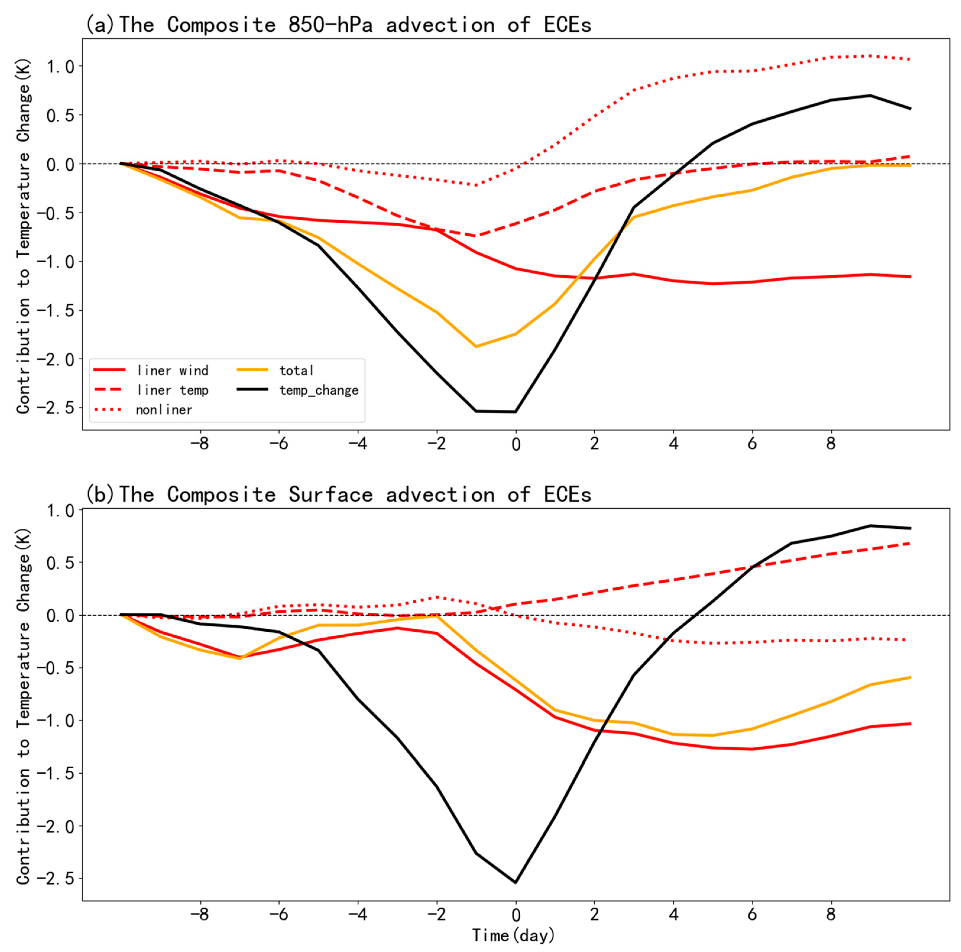
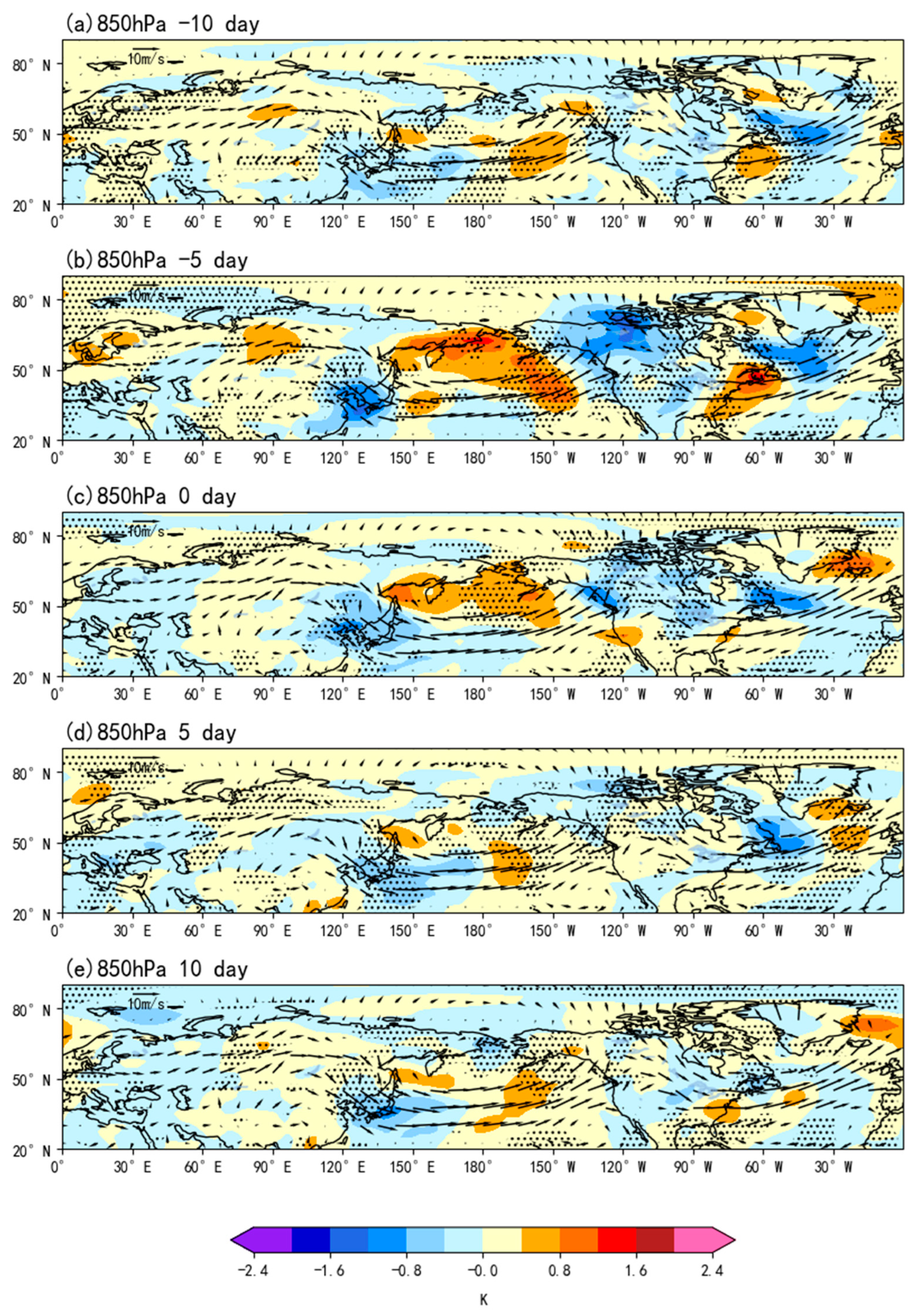
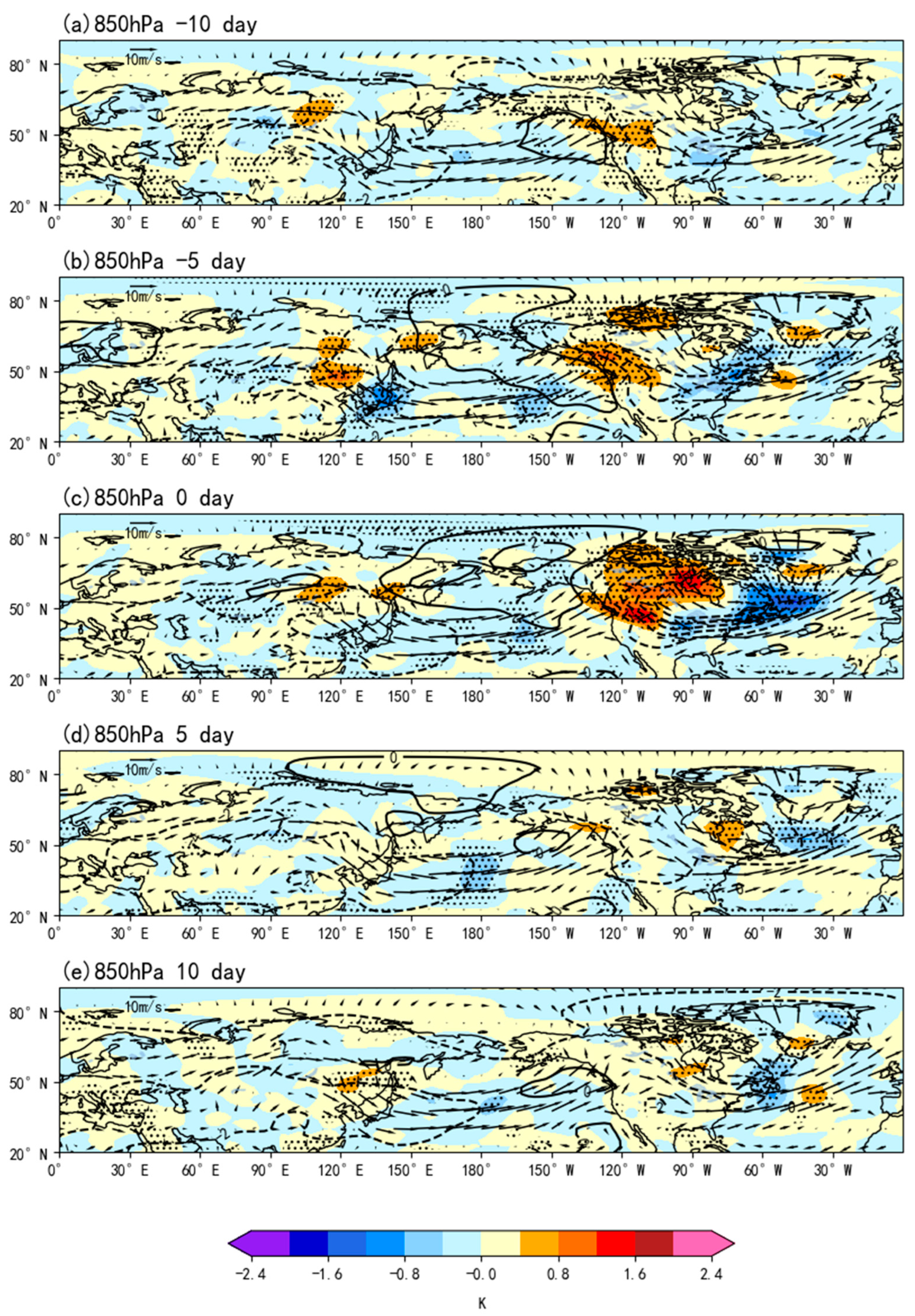
3.2. The Temperature Advection on the Surface and 850 hPa in ECEs

From Figure 7a, it can be observed that at 850 hPa, the pattern on day −5 appears closer to the WH circulation, while the correlation on day 0 is weaker. However, the temperature still reaches its coldest point only on day 0, which may be due to the faster development of weather processes in the lower troposphere, resulting in a shorter duration of the WH signal. The low-pressure system at 850 hPa (Figure 7a) is located further north compared to that at 500 hPa, and on day −5, this low-pressure system can be seen reaching Europe. Therefore, there remains an issue in the horizontal distribution that cannot be fully explained by the geopotential height. Using the research results from Clark and Feldstein [23], the advection results at 500 hPa, 850 hPa, and the surface are analyzed in ECEs. Only the surface and 850 hPa results are presented in this paper (Figure 9). “Total” denotes the sum of the linear wind, linear temperature, and nonlinear factors, while “temperature change” refers to the variation in temperature from one day to the next during ECEs. For the ECEs caused by WH, the main factor controlling temperature changes is the linear wind. The nonlinear and the linear temperature have comparable effects. Although the linear wind is only 1 K higher than the other two factors in the advection calculation, its contribution to the advective cooling accounts for 90%. The most significant cooling phase is concentrated from day −2 to day +4. When compared to the temperature change, the cooling actually begins on day −5. With the enhancement of the stationary wave in the early stage [18], the subtropical low pressure and the mid-latitude high-pressure ridge strengthen, leading to a significant enhancement of the linear wind under this influence (Figure 9). The linear wind at 850 hPa (Figure 10) clearly shows the cooling effect on North America caused by the northerly wind influenced by the abnormally strong ridge (Figure 6a) in the northwest of North America. Starting from day −5, the cold advection begins to affect a large area in the northern part of North America. This result is also consistent with our previous research on temperature anomaly. This could be due to the frequent disturbances at the surface weather scale, which lead to rapid temperature changes at the surface. The temperature drops significantly in a very short period of time and then gradually recovers.

Figure 10 and Figure 11 show the advection map of the linear wind and anomalous temperature. The results presented in Figure 11 are consistent with the temperature variation processes shown in Figure 6 and Figure 7. As early as day −5, we can observe an abnormally negative linear wind emerging from the Beaufort Sea and entering the northern side of the North American continent (Figure 10). Through the transport of cold advection, a large area of low linear wind values appears on day 0. This distribution also explains the widespread temperature drop in the temperature field of ECEs (Figure 6b), and even five days later, the North American continent is still affected by the linear wind. Regarding the variation in the linear temperature term, we believe it is interfered with some extent by the linear wind field, as the cooling region in the linear wind field on day −5 aligned well with the cooling region in the linear temperature on day 0, which may indicate a certain lag in the temperature field. However, the impact of the anomalous term on the temperature dropping of the ECEs studied can be neglected. Our result of CAM (Figure 12a) also provides sufficient evidence that this anomalous ridge is the main cause of guiding cold air propagation at different tropospheric levels. The NHC (Figure 12b) also demonstrates the characteristic of cold airflow being steered by the Greenland and Rocky Mountains. During the extremely cold weather associated with the WH pattern, the entire troposphere is consistently influenced by polar air masses. In summary, the occurrence and development of ECEs are caused by these tropospheric anomalies and the propagation of longwave signals.

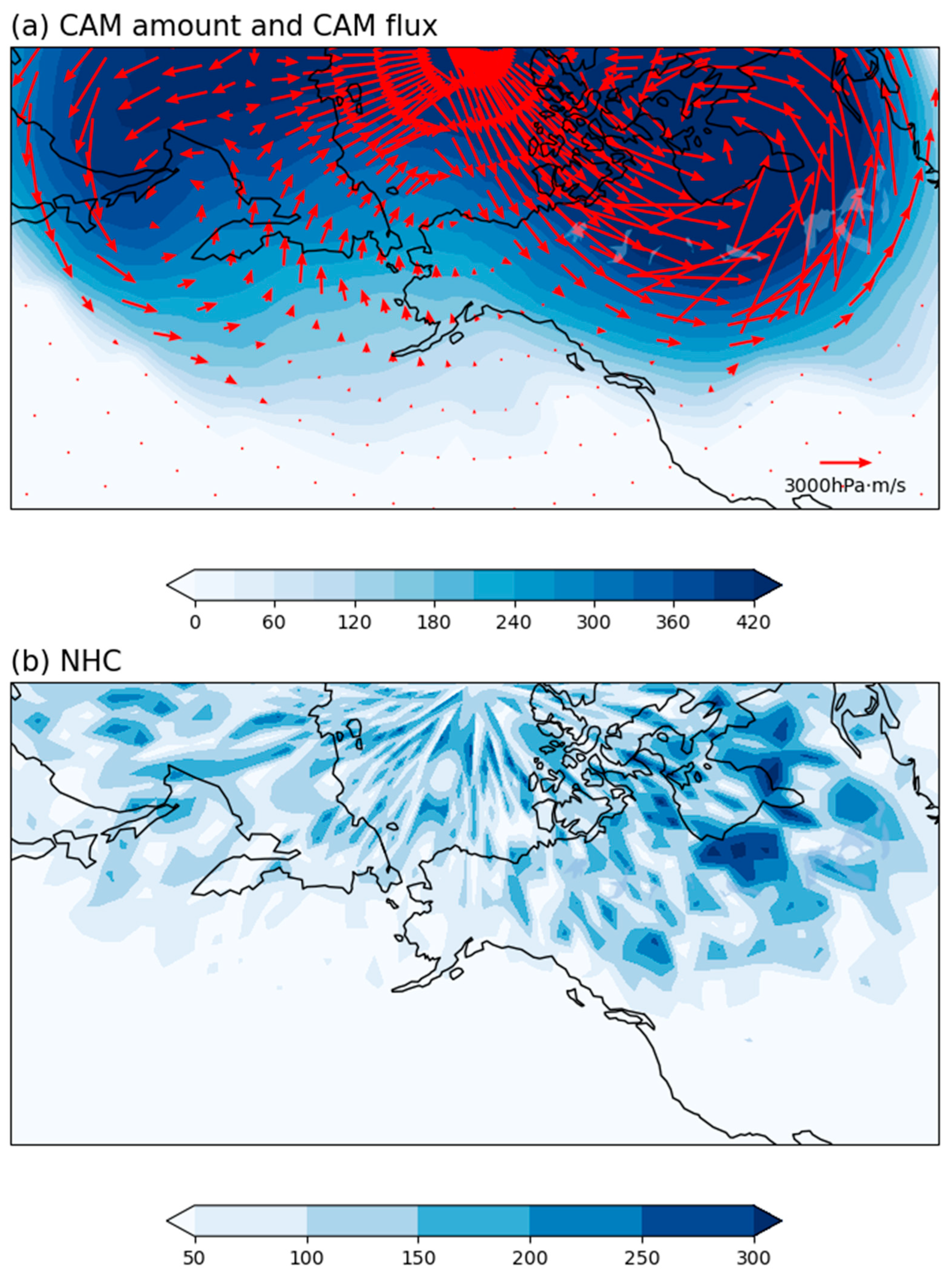
3.3. CAM Flux and NHC in ECEs

Previous studies have shown that extremely cold weather in North America results from the combined effects of horizontal transport and vertical flux [11,25]. Figure 12 shows the cold air mass flux calculated for ECEs using Equation (6). During the WH extreme cold weather, the largest cold air mass appears in the middle troposphere of the Arctic, which is consistent with the research results of Ivasaki [25]. Analysis of changes in the Negative Heat Content (NHC) reveals that distinct cold air masses originate from the Arctic flow toward the northern regions of North America (Figure 12b). Based on the characteristics of the cold air mass (CAM) flux (Figure 12a), the cold air from the Arctic is significantly influenced by the underlying surface. The ocean weakens the intensity of the cold air during winter. After reaching the continent, the air mass continues to be affected by cold advection as its movement progresses from north to south into the inland regions as the anomalous trough and ridge propagate. The cold air tends to accumulate in the northern part of North America before being rapidly transported to the mid- and high-latitude regions of the continent under the influence of strong mid-latitude westerly jet streams.

Through CAM flux (Figure 12a), the vertical and horizontal contributions of North American cold air and its associated anomalies can be clearly observed. These results are consistent with the earlier analysis of 500 hPa and 850 hPa fields. The NHC reflects the vertical temperature structure of CAM, and the cold air outbreak in North America is also influenced by the low-pressure trough overlying the region, coupled with blocking phenomena in the North Pacific and North Atlantic. This results in deepening troughs downstream of North America and ridges over Alaska, causing surface anticyclones to move southeastward [35]. The anomaly over Alaska, driven by Pacific blocking, enables the ridges in the early stages of WH extremely cold weather to sustain the southward movement of polar cold air masses. Because NHC is more susceptible to heat loss or absorption due to terrain or underlying surface properties, it exhibits a discontinuous characteristic; the accumulation of cold air over Greenland is significantly greater than that over the ocean surface. Combining the results of Figure 6 and Figure 7, the temperature drop observed from day −5 indicates that the cold air distribution represented by CAM aligns with the temperature changes in North America. This confirms that the source of the ECEs we identified indeed originates from Arctic cold air masses. Under the Influence of CAM flux, these cold air masses are transported from the Arctic to southern North America along with cyclonic systems. Based on the results of horizontal temperature advection, during the day 0 phase, interference from anomalous winds caused this cold air mass to spread across the mid-to-high latitude regions of North America.

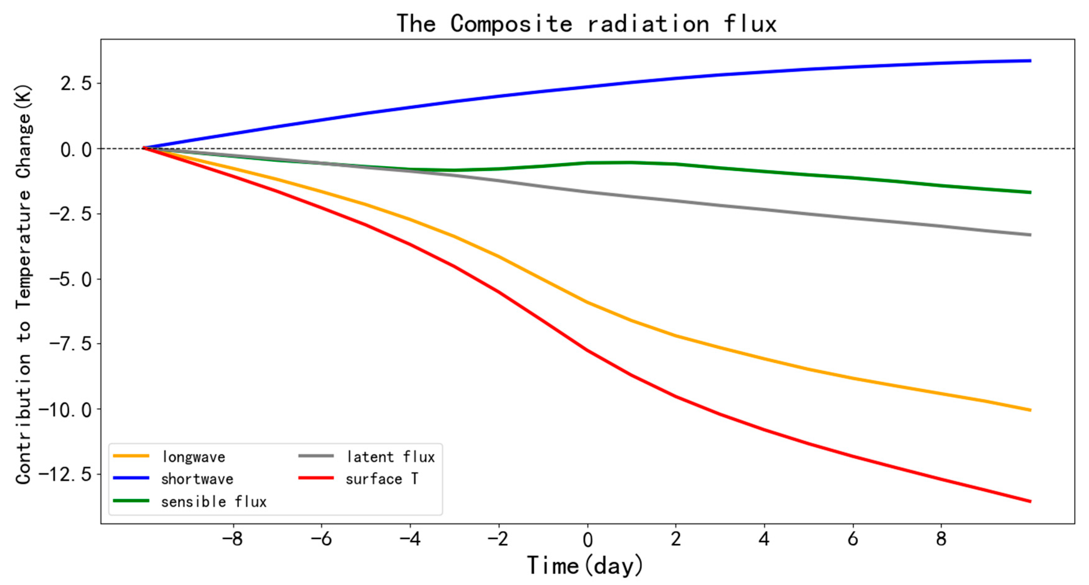
3.4. The Surface Energy Budget

The coupling relationship between longwave radiation and temperature during ECE performs well. Figure 13 shows significant sensible and latent heat fluxes on the western side of the Atlantic Ocean. Among all the terms in the surface energy budget, the downward longwave radiation anomaly most closely resembles the surface temperature anomaly, as shown in Figure 14. According to research by Luo et al. [36], this implies that downward longwave radiation plays a critical role in influencing near-surface temperatures during ECEs. Although longwave radiation can be influenced by various atmospheric conditions, the results in Figure 14 indicate that it closely follows changes in surface temperature. Compared with the air over the ocean, these heat fluxes exhibit smaller variations over land due to the stable stratification of the air over land. According to Clark and Feldstein [23], the spatial distribution of sensible and latent heat fluxes is balanced, indicating the formation of the vertical temperature contrast between the air and the ocean surface also leads to changes in the pressure gradient, resulting in the formation of strong westerly winds. The sensible and latent heat fluxes are partially balanced by the residual term $∆R-∆G$, which is attributed to other residual processes contained within the oceanic boundary layer. In summary, when WH anomalies induce linear winds leading to a temperature drop in North America, a strong vertical temperature gradient forms near the surface over the Atlantic Ocean (Figure 13). Because the ocean’s temperature remains relatively constant compared with the atmosphere and the land has a smaller heat capacity than the ocean, large temperature gradients do not develop over the land near the Atlantic. Therefore, the anomalous sensible and latent heat fluxes shown in Figure 13 develop over the ocean but not over the land; the temperature gradient between land and sea becomes the outlet of cold air moving out of the continent, so the results of ECEs (Figure 6b, Figure 7b and Figure 10) show that there is a strong cooling phenomenon in Newfoundland and its adjacent oceans.

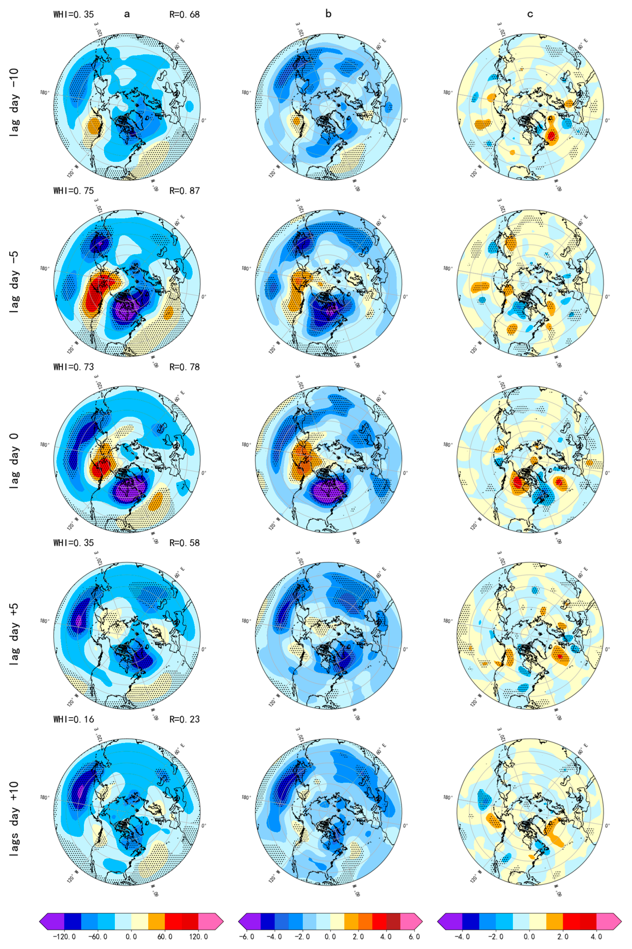
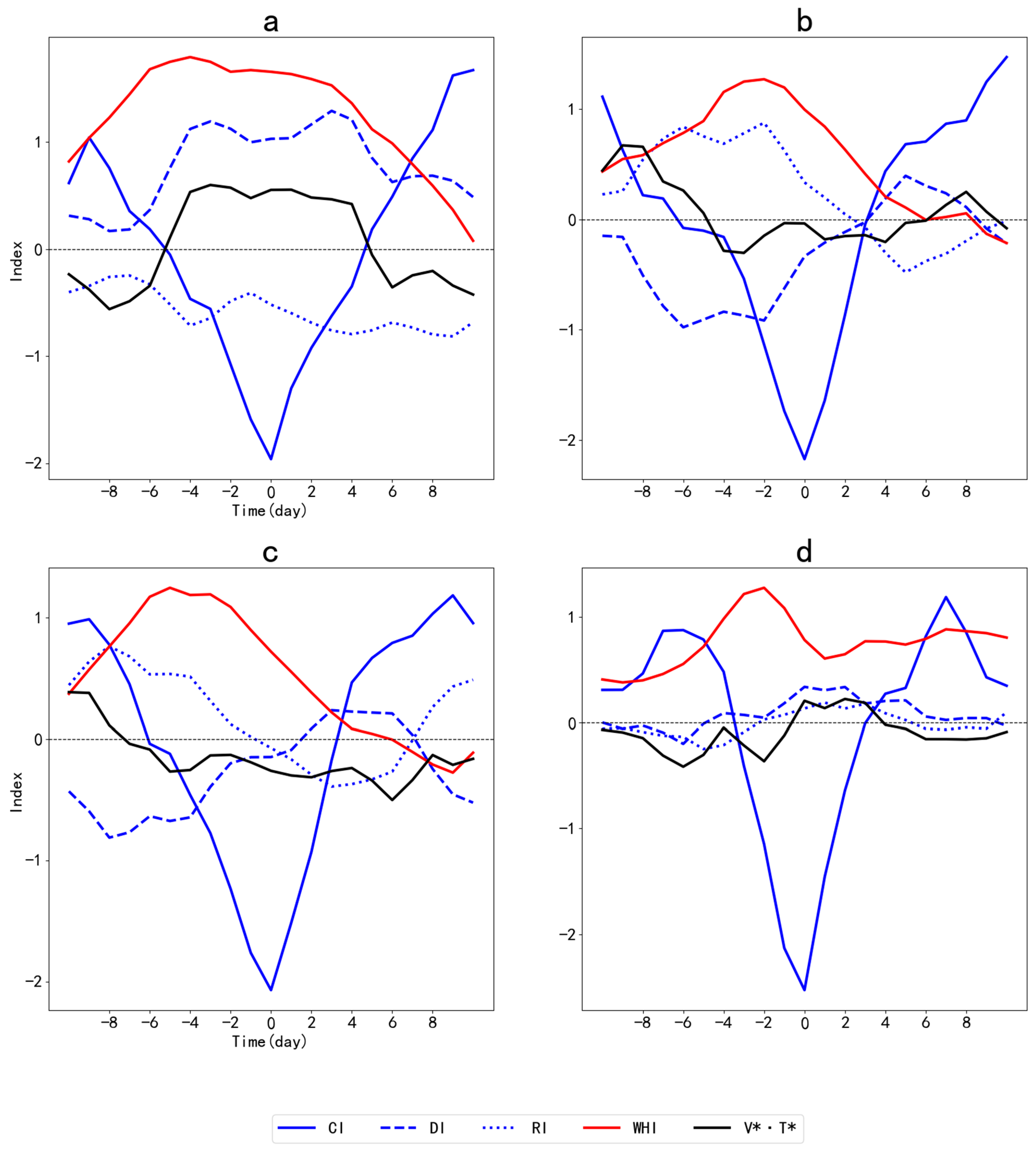
4. SOM Result of ECEs at 500 hPa and Stratospheric Diagnosis

Through comparative analysis of multiple clustering results, the geopotential height anomalies of ECEs were ultimately categorized into four distinct types. These types are differentiated by the distribution patterns of troughs and ridges, specifically the North American–North Atlantic Oscillation (NA-NAO) type (Figure 15a), the North Asian Ridge type (Figure 15b), the Atlantic Ridge type (Figure 15c), and the European Ridge–North Asian Trough type (Figure 15d). Regarding the variations in troughs and ridges over North Asia (Figure 15b,d), the results from the CAM analysis indicate that cold air masses propagating from the Arctic not only influence North America but also exhibit a branch flowing toward the Asian region (not shown in Figure 12). This phenomenon has also been noted in previous studies [25,27], with a significant proportion of North Asian anomalous signals observed. It is reasonable to infer that during ECEs, the cold air flowing toward Asia similarly affects the distribution of troughs and ridges in the mid-to-high latitude regions of Asia, leading to such anomalous circulation patterns. As for the other two types (Figure 15a,c), their anomalous trough-ridge distributions align more closely with conventional WH circulation anomalies. The NA-NAO type is characterized by the eastward propagation of anomalous North American troughs, resulting in a circulation pattern resembling the NAO. On the other hand, the Atlantic Ridge type arises from the northward expansion of the North American trough, allowing the anomalous ridge southeast of North America to extend northward, thereby forming continuous trough-ridge anomalies in the mid-to-high latitudes. Although this study categorized the results into four types, they essentially represent different developmental pathways of the North American trough and the North Asian trough-ridge patterns. If grouped into two broader categories (a&c and b&d), it becomes evident that the frequencies of these two circulation anomalies are comparable.

Previous studies [18,19] have shown that the WH mode typically influences the stratosphere through upwelling signals. Tan [20] pointed out that WH circulation anomaly may cause the displacement of the stratospheric polar vortex. Morevoer, this paper further analyzed the possible wave phenomena in WH circulation anomaly by classification to explain the tropospheric weather process. There is a difference in the total meridional mean between upward and downward propagation. Therefore, we used the downwelling index to assess whether the stratosphere impacts the WH troposphere and the reflection index to determine whether this signal represents an Alaskan tropospheric signal reflecting back to the North American continent. Based on the SOM results in Figure 15, the findings (Figure 16) indicate that approximately 90% of the signals in ECEs originate from the Alaska and North American regions.

From the perspective of stratospheric wave signals, both the North Asian Ridge type (Figure 16b) and the Atlantic Ridge type (Figure 16c) exhibit relatively clear reflection signals during the early stages of ECEs. This indicates that when these two types of circulation anomalies occur, stratospheric waves often propagate upward from the Alaska region to North America and then reflect back. As a result, the duration of WH circulation anomalies tends to be shorter, as evidenced by the decline in the WHI index following the decrease in the reflection index. In contrast, the NA-NAO type (Figure 16a) and the North Asian Trough type (Figure 16d) exhibit different characteristics. Anomalies in the downwelling index are observed, which is attributed to the upward-propagating wave signals in the stratosphere over North America during these two types of circulation anomalies. This leads to the dominant feature of upward-propagating waves throughout the stratosphere. Consequently, a strong coupling relationship is observed between the eddy heat flux and the downwelling index. Additionally, this suggests that during the occurrence of these two types of anomalies, the propagation efficiency of stratospheric waves is faster, resulting in a longer persistence of WH circulation anomalies. This is reflected in the slower decay rate of the WHI index compared with the other two types. In summary, stratospheric waves may influence the development of tropospheric weather processes, but the specific mechanisms require further investigation.

5. Summary and Discussion

In this paper, the association between the extremely cold weather in North America and the WH pattern is revealed using the NCEP/NCAR daily reanalysis datasets. The WH pattern is the tropospheric circulation, which dominates the ECEs over North America. As the growth of the WH pattern, the cold anomalies over North America strengthen and result in the extremely cold event. During the WH events, the stationary wave propagating from the eastern Pacific on day −10 causes a ridge anomaly in the Gulf of Alaska. The trough anomaly that appears over Greenland allows Arctic cold air to enter the northern part of North America. Starting from day −6, the ridge in the Gulf of Alaska intensifies, and the cold air penetrates deep into the North American continent. From day +2, the wave train began to deepen the trough in the eastern part of North America, and the “cold stream” was transported towards Newfoundland Island. In the later stages (after day +3), influenced by the Atlantic trough anomaly, the cold air crossed over the Atlantic. However, the NHC indicated that the intensity of this cold air would weaken, resulting in a relatively low level of coldness in Europe during the later stage of WH.

By analyzing the thermodynamic equation, the main temperature advection term leading to the cooling of North America is the advection of climate temperature by wind anomalies associated with the WH. The anomalous wind dominates the southward movement of cold air in the polar region and also leads to the accumulation of cold air mass on the North American continent, resulting in the outbreak of cold air through the fluctuation of anomalous troughs and ridges. The surface energy budget indicates that downward longwave radiation is the critical physical process in influencing near-surface temperatures during ECEs. The research on the temperature presented in this paper is limited. Previous works indicate that the ocean process, including the sea-ice-atmosphere interaction, could influence atmospheric teleconnection. This is also the physical process, which can be discussed in further research on the relationship between the WH and the ECEs.

The results of SOM indicate that upward Rossby waves over the northern area of North America can be evident for some extremely cold weather cases associated with the long-lasting WH pattern (Figure 15a). The downward phenomenon indicated by DI is mostly evident prior to the central date of ECEs (Figure 16b,c). However, the vertical propagation of Rossby waves is inapparent during about 25% of ECEs (Figure 16d). Within several months after the attenuation of the polar vortex in the stratosphere, ECEs are more likely to occur in North America, Northern Europe, and mid-to-high latitude regions of Asia [37,38]. According to our results, the relationship between ECEs influenced by WH and the stratosphere is not as apparent as that between NAO or NAM and the stratosphere. Changes in the polar vortex in the stratosphere are usually precursors for identifying extremely cold weather. The relationship between the WH and the stratosphere polar vortex is discussed in previous works [18,20]. The WH circulation will enhance wave-2 and suppress wave-1 fluxes upward into the stratosphere, resulting in the shift of the stratospheric polar vortex to North America. The analysis of the stratosphere presented in this paper is also relatively limited, which needs further investigation in the future.

References

1. Forbes, G.S.; Thomson, D.W.; Anthes, R.A. Synoptic and Mesoscale Aspects of an Appalachian Ice Storm Associated with Cold-Air Damming. Mon. Weather Rev. 1987, 115, 564–591. [Google Scholar] [CrossRef]
2. Boberg, F.; Lundstedt, H. Solar wind electric field modulation of the NAO: A correlation analysis in the lower atmosphere. Geophys. Res. Lett. 2003, 30, 1825. [Google Scholar] [CrossRef]
3. Notaro, M.; Wang, W.-C.; Gong, W. Model and Observational Analysis of the Northeast U.S. Regional Climate and Its Relationship to the PNA and NAO Patterns during Early Winter. Mon. Weather Rev. 2006, 134, 3479–3505. [Google Scholar] [CrossRef]
4. Swanson, K.L.; Tsonis, A.A.; Wang, G. On the Role of Atmospheric Teleconnections in Climate. J. Clim. 2008, 21, 2990–3001. [Google Scholar]
5. Jung, T.; Vitart, F.; Ferranti, L.; Morcrette, J.-J. Origin and predictability of the extreme negative NAO winter of 2009/10. Geophys. Res. Lett. 2011, 38, L07701. [Google Scholar] [CrossRef]
6. Black, R.; Barlow, M.; Gershunov, A.; Lee, Y.-Y.; Leung, R.; Gyakum, J.R.; Grotjahn, R.; Gutowski, W.J.; Lim, Y.-K.; Bosilovich, M.; et al. North American extreme temperature events and related large scale meteorological patterns: A review of statistical methods, dynamics, modeling, and trends. Clim. Dyn. 2015, 46, 1151–1184. [Google Scholar]
7. Shen, X.; Liu, B.; Lu, X. Weak Cooling of Cold Extremes Versus Continued Warming of Hot Extremes in China During the Recent Global Surface Warming Hiatus. J. Geophys. Res. Atmos. 2018, 123, 4073–4087. [Google Scholar] [CrossRef]
8. Lemus-Canovas, M. Changes in compound monthly precipitation and temperature extremes and their relationship with teleconnection patterns in the Mediterranean. J. Hydrol. 2022, 608, 127580. [Google Scholar] [CrossRef]
9. Folland, C.K.; Knight, J.R.; Vallis, G.K.; Scaife, A.A. A stratospheric influence on the winter NAO and North Atlantic surface climate. Geophys. Res. Lett. 2005, 32, L18715. [Google Scholar] [CrossRef]
10. Portis, D.H.; Walsh, J.E.; Rauber, R.M.; Cellitti, M.P. Extreme cold air outbreaks over the United States, the polar vortex, and the large-scale circulation. J. Geophys. Res. Atmos. 2006, 111, D02114. [Google Scholar] [CrossRef]
11. Turner, J.K.; Gyakum, J.R. The Development of Arctic Air Masses in Northwest Canada and Their Behavior in a Warming Climate. J. Clim. 2011, 24, 4618–4633. [Google Scholar] [CrossRef]
12. Hitchcock, P.; Simpson, I.R. The Downward Influence of Stratospheric Sudden Warmings. J. Atmos. Sci. 2014, 71, 3856–3876. [Google Scholar] [CrossRef]
13. Baldwin, M.P.; Scaife, A.A.; Hardiman, S.C.; Kidston, J.; Butchart, N.; Mitchell, D.M.; Gray, L.J. Stratospheric influence on tropospheric jet streams, storm tracks and surface weather. Nat. Geosci. 2015, 8, 433–440. [Google Scholar]
14. Thompson, D.W.J.; Wallace, J.M. The Arctic oscillation signature in the wintertime geopotential height and temperature fields. Geophys. Res. Lett. 1998, 25, 1297–1300. [Google Scholar] [CrossRef]
15. Foster, J.; Barlow, M.; Saito, K.; Cohen, J.; Jones, J. Winter 2009–2010: A case study of an extreme Arctic Oscillation event. Geophys. Res. Lett. 2010, 37, L17707. [Google Scholar] [CrossRef]
16. Baxter, S.; Nigam, S. Key Role of the North Pacific Oscillation–West Pacific Pattern in Generating the Extreme 2013/14 North American Winter. J. Clim. 2015, 28, 8109–8117. [Google Scholar] [CrossRef]
17. Van Oldenborgh, G.J.; Haarsma, R.; De Vries, H.; Allen, M.R. Cold Extremes in North America vs. Mild Weather in Europe: The Winter of 2013–14 in the Context of a Warming World. Bull. Am. Meteorol. Soc. 2015, 96, 707–714. [Google Scholar] [CrossRef]
18. Hartmann, D.L.; Ceppi, P.; Bao, M.; Tan, X. The Role of Synoptic Waves in the Formation and Maintenance of the Western Hemisphere Circulation Pattern. J. Clim. 2017, 30, 10259–10274. [Google Scholar]
19. Bao, M.; Wallace, J.M. Cluster Analysis of Northern Hemisphere Wintertime 500-hPa Flow Regimes during 1920–2014. J. Atmos. Sci. 2015, 72, 3597–3608. [Google Scholar] [CrossRef]
20. Tan, X.; Bao, M. Linkage Between a Dominant Mode in the Lower Stratosphere and the Western Hemisphere Circulation Pattern. Geophys. Res. Lett. 2020, 47, e2020GL090105. [Google Scholar] [CrossRef]
21. Kanamitsu, M.; Ebisuzaki, W.; Woollen, J.; Yang, S.-K.; Hnilo, J.J.; Fiorino, M.; Potter, G.L. NCEP–DOE AMIP-II Reanalysis (R-2). Bull. Am. Meteorol. Soc. 2002, 83, 1631–1644. [Google Scholar] [CrossRef]
22. Quiroz, R.S. The Climate of the 1983–84 Winter—A Season of Strong Blocking and Severe Cold in North America. Mon. Weather Rev. 1984, 112, 1894–1912. [Google Scholar] [CrossRef]
23. Clark, J.P.; Feldstein, S.B. What Drives the North Atlantic Oscillation’s Temperature Anomaly Pattern? Part I: The Growth and Decay of the Surface Air Temperature Anomalies. J. Atmos. Sci. 2020, 77, 185–198. [Google Scholar] [CrossRef]
24. Iwasaki, T.; Mochizuki, Y. Mass-Weighted Isentropic Zonal Mean Equatorward Flow in the Northern Hemispheric Winter. Sola 2012, 8, 115–118. [Google Scholar] [CrossRef]
25. Takaya, K.; Sawada, M.; Ujiie, M.; Shoji, T.; Iwasaki, T.; Kanno, Y. Isentropic Analysis of Polar Cold Airmass Streams in the Northern Hemispheric Winter. J. Atmos. Sci. 2014, 71, 2230–2243. [Google Scholar]
26. Iida, M.; Sugimoto, S.; Suga, T. Severe Cold Winter in North America Linked to Bering Sea Ice Loss. J. Clim. 2020, 33, 8069–8085. [Google Scholar] [CrossRef]
27. Abdillah, M.R.; Kanno, Y.; Iwasaki, T. Tropical–Extratropical Interactions Associated with East Asian Cold Air Outbreaks. Part I: Interannual Variability. J. Clim. 2017, 30, 2989–3007. [Google Scholar] [CrossRef]
28. Nishii, K.; Nakamura, H.; Orsolini, Y.J. Geographical Dependence Observed in Blocking High Influence on the Stratospheric Variability through Enhancement and Suppression of Upward Planetary-Wave Propagation. J. Clim. 2011, 24, 6408–6423. [Google Scholar] [CrossRef]
29. Ueda, M.; Mukougawa, H.; Maury, P.; Claud, C.; Kodera, K. Absorbing and reflecting sudden stratospheric warming events and their relationship with tropospheric circulation. J. Geophys. Res. Atmos. 2016, 121, 80–94. [Google Scholar]
30. Hewitson, B.C.; Crane, R.G. Consensus between GCM climate change projections with empirical downscaling: Precipitation downscaling over South Africa. Int. J. Climatol. 2006, 26, 1315–1337. [Google Scholar] [CrossRef]
31. Arritt, R.W.; Gutowski, W.J.; Otieno, F.O.; Pan, Z.; Takle, E.S. Diagnosis and Attribution of a Seasonal Precipitation Deficit in a U.S. Regional Climate Simulation. J. Hydrometeorol. 2004, 5, 230–242. [Google Scholar]
32. Cassano, E.N.; Uotila, P.; Cassano, J.J.; Lynch, A.H. Predicted changes in synoptic forcing of net precipitation in large Arctic river basins during the 21st century. J. Geophys. Res. Biogeosci. 2007, 112, G04S49. [Google Scholar] [CrossRef]
33. Gong, T.; Feldstein, S.; Lee, S. The Role of Downward Infrared Radiation in the Recent Arctic Winter Warming Trend. J. Clim. 2017, 30, 4937–4949. [Google Scholar] [CrossRef]
34. Gong, T.; Screen, J.A.; Simmonds, I.; Lee, S.; Feldstein, S.B. Revisiting the Cause of the 1989–2009 Arctic Surface Warming Using the Surface Energy Budget: Downward Infrared Radiation Dominates the Surface Fluxes. Geophys. Res. Lett. 2017, 44, 10654–10661. [Google Scholar] [CrossRef]
35. Marinaro, A.; Hilberg, S.; Changnon, D.; Angel, J.R. The North Pacific–Driven Severe Midwest Winter of 2013/14. J. Appl. Meteorol. Climatol. 2015, 54, 2141–2151. [Google Scholar] [CrossRef]
36. Zhong, L.; Luo, B.; Luo, D.; Wu, L.; Simmonds, I. Atmospheric circulation patterns which promote winter Arctic sea ice decline. Environ. Res. Lett. 2017, 12, 054017. [Google Scholar] [CrossRef]
37. Thompson, D.W.J.; Baldwin, M.P.; Wallace, J.M. Stratospheric Connection to Northern Hemisphere Wintertime Weather: Implications for Prediction. J. Clim. 2002, 15, 1421–1428. [Google Scholar] [CrossRef]
38. Kolstad, E.W.; Breiteig, T.; Scaife, A.A. The association between stratospheric weak polar vortex events and cold air outbreaks in the Northern Hemisphere. Q. J. R. Meteorol. Soc. 2010, 136, 886–893. [Google Scholar] [CrossRef]
Figure 1. The 500 hPa WH pattern from Bao and Wallace (2015), the contour interval is 25 m; red (blue) contours denote positive (negative) values, the zero contours are omitted.
Atmosphere 16 00781 g001
Figure 2. The extreme temperature anomaly at surface level in the 1979 and 2023 winter. The black box denotes the selected region (45° N to 65° N, 115° W to 50° W) used to define the extremely cold event.
Atmosphere 16 00781 g002
Figure 3. Distributions of ECEs and WH events between the 1979 and 2023 winters. The solid black lines denote the ECEs. The red dot denotes the WH events. The x-axis denotes the months and days of each winter. The x-axis denotes the winter months and days of each winter. The y-axis denotes the years. The December in the x-axis corresponds to December of last year.
Atmosphere 16 00781 g003
Figure 4. The eddy heat flux at 100 hPa, which used climatic V*·T*. The two boxes indicate the regions where DI and RI are calculated. One region is 50° N~75° N, 150° E~160° W. Another region is 60° N~85° N, 80° W~130° W, and it also denotes the downwelling index. The difference between these two regions shows the reflection index.
Atmosphere 16 00781 g004
Figure 5. The composite result of the WH event at 500 hPa. (From left to right) Columns display composite anomalies of (a) 500 hPa geopotential height. Rows display time lags; the WHI is provided on the top-left hand, and the correlation coefficient is on the top-right. And the lower troposphere temperature field: (b) temperature anomalies (units: K) at surface level, (c) temperature anomalies (units: K) at 850 hPa. The dotted area represents the region that has passed the 95% confidence test.
Atmosphere 16 00781 g005
Figure 6. Composite result of WH Extreme Cold Events at 500 hPa. Columns display composite anomalies of (a) 500 hPa geopotential height of ECEs, (b) temperature (units: K) of ECEs at 500 hPa, and (c) temperature variation (units: K) of ECEs at 500 hPa. Rows display time lags. Day 0 corresponds to the day with the highest CI of each field. The dotted area represents the region that has passed the 95% confidence test.
Atmosphere 16 00781 g006
Figure 7. Composite result of WH Extreme Cold Events at 850 hPa. Columns display composite anomalies of (a) 850 hPa geopotential height of ECEs, (b) temperature (units: K) of ECEs at 850 hPa, and (c) temperature variation (units: K) of ECEs at 500 hPa. Rows display time lags. Day 0 corresponds to the day with the highest CI of each field. The dotted area represents the region that has passed the 95% confidence test.
Atmosphere 16 00781 g007
Figure 8. The redefined composite results of the indices. The blue line denotes the composite result WHI during ECEs, the red line denotes the result CI at 850 hPa during WH events, the green line denotes the CI, and the orange line denotes the WHI. The vertical axis shows the normalized values, and the horizontal axis represents time.
Atmosphere 16 00781 g008
Figure 9. The composite advection on the lowest surface, the regions indicated by Figure 3. The solid red line denotes the ( u · T ¯ + u · T ¯ ¯ ) , which shows the linear wind field, and the dashed red line denotes the ( u ¯ · T + u ¯ · T ¯ ) , which shows the linear temperature field, and the dotted red line denotes the ( u · T + u · T ¯ ) , which shows the nonlinear field. The orange line denotes the total contribution to the temperature variation by the temperature advection. The black line denotes the temperature variation in extreme cold events. The upper panel shows the composite results for 850 hPa level; the lower panel shows the results for the surface level. Both the x-axis denotes the lag day of the ECEs.
Atmosphere 16 00781 g009
Figure 10. Daily composite of the 850 hPa u · T ¯ + u · T ¯ ¯ for lag days of the WH extreme cold event. Shading indicates the u · T ¯ + u · T ¯ ¯ , the arrows show the climatological wind and the scaling of arrows is given at top-left. Day 0 corresponds to the day with the highest CI of each field. The same as below. The dotted area represents the region that has passed the 95% confidence test.
Atmosphere 16 00781 g010
Figure 11. Daily composite of the 850 hPa u ¯ · T + u ¯ · T ¯ for lag days of the WH extreme cold event. Contour denotes the temperature anomaly (interval: 2 °C), the line denotes positive, and the dashed denotes negative. Shading indicates the u ¯ · T + u ¯ · T ¯ , the arrows show the climatological wind and the scaling of arrows is given at the top-left. The dotted area represents the region that has passed the 95% confidence test.
Atmosphere 16 00781 g011
Figure 12. (a) CAM amount and CAM flux, (b) NHC in the ECEs. The CAM amount and flux are shown where located at 40° N~90° N, 120° E~60° W. The shadow in (a) denotes the CAM amount and in (b) denotes the NHC; the red arrows in (a) show the cold air mass flux. The flux at the North Pole can be neglected.
Atmosphere 16 00781 g012
Figure 13. Surface energy budget composite during the ECEs. Columns denote anomalies of downward longwave radiation, net shortwave radiation, sensible heat flux, latent heat flux, and the residual term. Rows denote time lags. All terms are normalized by the quantity 4 σ ε s { T s } 3 , which ensures that their units are kelvins. The dotted area represents the region that has passed the 95% confidence test.
Atmosphere 16 00781 g013
Figure 14. The composite radiation flux on the surface level, the regional average is the same as that for ECEs (45° N to 65° N, 115° W to 55° W). The red line indicates the surface temperature, the yellow line indicates longwave radiation, the blue line indicates shortwave radiation, the green line indicates the sensible flux and the gray line indicates the latent flux. All terms are normalized by 4 σ ε s { T s } 3 .
Atmosphere 16 00781 g014
Figure 15. Composite 500 hPa geopotential height for the first four SOM clusters in ECEs, (ad) denotes the first, second, third, and fourth SOM clustering type. The top-right shows the number of clustering members. The top-left corner is the RI (top) and DI (bottom). The black solid line is the Alaska stratosphere region (50° N~75° N, 150° E~160° W) mentioned in the method, and the red solid line is the American stratosphere region (60° N~85° N, 130° W~80° W).
Atmosphere 16 00781 g015
Figure 16. Composite 100 hPa index of the cluster derived from SOM. (ad) are the first, second, third, and fourth SOM clustering members in ECEs. The lead and lag distribution of various indices of the ECEs day 0: the blue solid line represents the cold index, the blue dashed line represents the downwelling index, the blue dotted line represents the reflex index, the black solid line represents the zonal mean at 100 hPa, and the red solid line represents the WHI. All results have been normalized.
Atmosphere 16 00781 g016
Disclaimer/Publisher’s Note: The statements, opinions and data contained in all publications are solely those of the individual author(s) and contributor(s) and not of MDPI and/or the editor(s). MDPI and/or the editor(s) disclaim responsibility for any injury to people or property resulting from any ideas, methods, instructions or products referred to in the content.