Wind Speed Forecasting in the Greek Seas Using Hybrid Artificial Neural Networks

Abstract

The exploitation of renewable energy is essential for mitigating climate change and reducing fossil fuel emissions. Wind energy, the most mature technology, is highly dependent on wind speed, and the accurate prediction of the latter substantially supports wind power generation. In this work, various artificial neural networks (ANNs) were developed and evaluated for their wind speed prediction ability using the ERA5 historical reanalysis data for four potential Offshore Wind Farm Organized Development Areas in Greece, selected as suitable for floating wind installations. The training period for all the ANNs was 80% of the time series length and the remaining 20% of the dataset was the testing period. Of all the ANNs examined, the hybrid model combining Long Short-Term Memory (LSTM) and Gated Recurrent Unit (GRU) networks demonstrated superior forecasting performance compared to the individual models, as evaluated by standard statistical metrics, while it also exhibited a very good performance at high wind speeds, i.e., greater than 15 m/s. The hybrid model achieved the lowest root mean square errors across all the sites—0.52 m/s (Crete), 0.59 m/s (Gyaros), 0.49 m/s (Patras), 0.58 m/s (Pilot 1A), and 0.55 m/s (Pilot 1B)—and an average coefficient of determination (R²) of 97%. Its enhanced accuracy is attributed to the integration of the LSTM and GRU components strengths, enabling it to better capture the temporal patterns in the wind speed data. These findings underscore the potential of hybrid neural networks for improving wind speed forecasting accuracy and reliability, contributing to the more effective integration of wind energy into the power grid and the better planning of offshore wind farm energy generation.

1. Introduction

The exploitation of renewable energy sources has become an important strategy for countries to mitigate the impacts of global warming and reduce emissions from fossil fuels [1]. Wind energy, being the most promising and technologically mature source of renewable energy globally [2], provides a great alternative for energy generation [3]. For the efficient operation of a wind farm, the accurate estimation and forecasting of the energy output from wind turbines and the effective integration of the wind energy production from the wind farm into the power grid are necessary, with the accurate prediction of wind speed being of the utmost importance.

The main challenge in wind speed forecasting is capturing and modeling the highly nonlinear and dynamic nature of wind patterns. Additionally, under the context of global climate change, the forecasting of extreme winds from tropical cyclones is becoming increasingly important for areas that are prone to such phenomena [4]. Accurate wind speed forecasting becomes particularly important in complex geographical regions like the Greek seas, where potential Offshore Wind Farm Organized Development Areas (OWFODAs) have been planned to be located relatively close to the shore (at distances less than 6 nm). Moreover, the Greek seas are known for their variable wind conditions, which can significantly impact wind power generation in the region. The complexity of wind patterns, influenced by various meteorological patterns, renders wind forecasting a challenging task. Yet, a variety of approaches have been suggested in the literature to address these difficulties.

Wind speed forecasting approaches are broadly classified into physics-based models, statistical models, artificial neural networks (ANNs), and hybrid models. The prediction time horizons vary from the short term (up to 8 h ahead), medium term (up to 24 h ahead), to long term (of the order of some days ahead) [5].

The physics-based models demand a strong theoretical foundation and substantial computational resources. They rely on physical data, such as atmospheric pressure, temperature, and topography, to forecast wind speeds, while the spatial and temporal resolution are important factors related to the particular application and the intended data use [6,7,8,9,10]. These physics-based models, developed primarily by meteorologists for broad-scale weather forecasting, may not offer the level of accuracy required for short-term and high-spatial-and-temporal-resolution wind speed forecasts, as they are time-consuming and expensive [11].

Numerous studies dedicated to developing robust wind speed prediction models have been conducted. Traditional wind speed forecasting methods, such as time series analyses and statistical approaches, often have some limitations in capturing the nonlinear and complex nature of wind patterns. Specifically, statistical models leverage historical wind speed measurements to forecast future wind speeds. These models work well overall for short-term predictions [12], and are computationally less intensive and do not require extensive physical information. Some common time series analysis models for wind speed forecasting are the autoregressive moving average (ARMA), Kolmogorov–Zurbenko filter models, and autoregressive integrated moving average models (ARIMA) [13]. Huang et al. [14] proposed an ARMA model to analyze and quantify the time-varying standard deviation of non-stationary wind speed data. Jeong et al. [15] developed a statistical post-processing technique to enhance the accuracy of numerical weather prediction models, while Soukissian and Karathanasi [16] applied various robust regression techniques for calibrating numerical model results and predicting wind speed more accurately. Ouarda et al. [17] used a statistical model that incorporated a wind speed predictor to address interannual variability. Galanis et al. [18] developed and evaluated a hybrid optimization framework that integrated Bayesian modeling and a nonlinear Kalman filter, which minimized the systematic bias and also constrained the variability in errors and the uncertainty in the predictions. However, statistical models also exhibit certain limitations, including reduced predictive accuracy for low-order models and challenges in estimating the parameters for high-order models. Additionally, statistical models are susceptible to converging to local optima when forecasting wind speed time series, which are complex, nonlinear, and stochastic in nature [13]. More literature on these techniques can be found in [9,19,20,21].

Artificial Neural Networks (ANNs) have also been implemented in order to capture the nonlinear and complex nature of wind patterns for more accurate wind speed forecasting. Some initial studies were based on the usage of feedforward neural networks (FFNs) for wind speed prediction [22]. These networks, trained using backpropagation algorithms, demonstrated the overall potential of ANNs for capturing wind patterns. Noorollahi et al. [23] investigated the use of ANNs for spatio-temporal wind speed forecasting in Iran. For temporal forecasting, three different ANN models, namely the Radial Basis Function Neural Network (RBFNN), Backpropagation Neural Network (BPNN), and Adaptive Neuro-Fuzzy Inference System (ANFIS), were used. These models were applied to real-life data to predict short-term wind speeds at three wind observation stations in Iran. Their results suggested that the BPNN and ANFIS performed similarly, while the RBFNN exhibited larger errors.

FFNs have limitations in handling temporal dependencies in wind data. To further improve the accuracy of wind forecasting and to overcome the limitations of FFNs, recurrent neural networks (RNNs) have been adopted, specifically Long Short-Term Memory (LSTM) [10,24] and a Gated Recurrent Unit (GRU) [25]. These architectures, with their memory mechanisms, are better suited for time series data like wind speed. Barbounis et al. [26] focused on using RNNs for long-term wind speed and wind power forecasting. The study used meteorological data as the input, specifically the wind speed and direction from numerical forecasts obtained from atmospheric modeling systems. The performance of the recurrent networks was compared to that of static models, like static multilayer perceptron (MLP) and finite impulse response multilayer perceptron, demonstrating the advantages of recurrent architectures for long-term wind forecasting.

While these individual machine learning models have shown promising results, there is increasing interest in developing hybrid models that can leverage the strengths of multiple techniques. This is because single models may also exhibit inherent limitations and may often be ill-equipped to handle the complex and stochastic characteristics of wind speed patterns [13,27]. Combined or hybrid models have been applied to wind speed forecasting and are expected to yield more accurate predictions compared to standalone models [28]. Some studies have proposed hybrid models that integrate ANNs with other techniques, such as the layer-stacking method, decomposition methods, and Fourier transformations to improve forecasting accuracy and stability [29,30,31]. Combining ANNs with statistical models like ARIMA may also improve forecasting accuracy by capturing both linear and nonlinear patterns [32]. Hybrid models incorporating deep learning techniques, such as convolutional neural networks (CNNs) along with RNNs, have also shown promising results [33]. Zhang et al. [34] proposed a hybrid model that combines a Variational Mode Decomposition of the wind speed; a wavelet transform; and a neural network ensemble incorporating a Principal Component Analysis, Radial Basis Function techniques, and backpropagation [35,36,37,38]. Liu et al. [39] developed a hybrid model for wind speed prediction that combines RNNs, Empirical Mode Decomposition (EMD, [40]), and the ARIMA model. The EMD method decomposes the original wind speed series into Intrinsic Mode Functions (IMFs) and a residual. Then, based on the complexity of each IMF measured by the sample entropy, either an LSTM or ARIMA model is used for prediction. High-complexity IMFs are predicted using LSTM, while low-complexity IMFs and residuals are predicted using the ARIMA model. This approach leverages the strengths of each model, with the LSTM and ARIMA models handling the nonlinear and non-stationary components and the more regular components of the wind speed series, respectively. Their results have demonstrated the effectiveness of a hybrid approach compared to using individual models. He et al. [13] proposed a probabilistic wind speed forecasting method integrating both LSTM and the Gaussian Mixture Model (GMM). Ref. [36] developed a new approach to wind speed forecasting that combines recurrent neural networks and a support vector machine (SVM). The framework uses a wavelet transform to disaggregate the original wind speed data into its constituent sub-series. Recurrent neural network architectures, such as standard RNNs, LSTM, and GRUs, are used to extract more complex temporal features from the low-frequency sub-series of the wind speed data. These extracted features are then fed into an SVM for prediction. The method has been applied to real-world data and demonstrated that hybrid models using RNNs and SVMs outperform traditional methods. Özbilge et al. investigated the use of deep recurrent neural network (DRNN) models for short-term wind speed forecasting, utilizing data from a wind platform to predict wind speeds one hour ahead [24]. Three types of recurrent layers were tested within the DRNN architecture, i.e., LSTM, GRU, and a simple RNN. Their results indicated a strong correlation between the actual and predicted wind speed for all the three recurrent layers. Jittratorn et al. detailed a very short-term wind power prediction model using a hybrid LSTM–Markov chain approach [41]. The key innovation was the incorporation of a wind speed correction mechanism before feeding the data into the LSTM network. This correction aimed to mitigate errors in the original wind speed data, leading to improved prediction accuracy. The study compared the hybrid model’s performance against several individual models, including a Random Forest, Support Vector Regression, LSTM, and Bi-directional GRU. Their results showed that the proposed hybrid model produced the lowest mean relative error ($MRE$), root mean squared error ($RMSE$), and normalized root mean squared error ($NRMSE$) compared to the other models. A recent review of the artificial intelligence models used for wind speed forecasting can be found in [42]. The effectiveness of any neural network depends on the accuracy of the data being trained. The observational data from wind measuring equipment offers the highest accuracy. However, failure in measurement leading to missing data is one of the shortcomings. In this sense, model data offers an alternative and some is publicly available. Dyukarev [43] in his research utilized the European Centre for Medium-Range Weather Forecasts’ (ECMWF’s ERA5) land reanalysis data using different neural networks to fill in the large and frequent gaps in the in situ data records of meteorological observations. Shikhovtsev et al. [44] focused on using neural networks to estimate and predict seeing, a key parameter of optical turbulence, at the Large Solar Telescope site using meteorological data obtained from ERA5. Some other researchers [45,46,47] have verified the accuracy of the ERA5 model data prior to its utilization by comparing it with the available observational data.

The Greek seas are considered one of the most favorable areas in the Mediterranean basin for the development of offshore wind farms (OWFs) [48,49]. Specifically, the Aegean Sea is one of the windiest areas, mainly due to the Etesian wind system that occurs every summer [50]. The development of OWFs is a national strategy to achieve the aims of meeting the European targets for the decarbonization of energy, providing energy security, and introducing “green” and affordable energy into the Greek energy mix. The Hellenic Parliament in 2022 passed L.4964/2022, which included all the relevant procedures for the development of OWFs in the Greek seas. Nominated by the Greek state, the Hellenic Hydrocarbons & Energy Resources Management Company SA (HEREMA) is responsible for the management of the research, investigation, and identification of potential Offshore Wind Farm Organized Development Areas (OWFODAs). In this context, in October 2023, a draft of the National Offshore Wind Farm Development Programme (NDP-OWF), along with the Strategic Environmental Impact Assessment (SEIA), was officially published by HEREMA, including, inter alia, the preliminary delimitation of the potential OWFODAs, as well as the initial estimation of the available installed capacity of each site [51]. In the medium-term horizon (2030–2032), ten potential OWFODAs were identified, mainly designed for floating installations, while two additional pilot projects were also included for the development of fixed-bottom OWF projects. In this study, four medium-term potential OWFODAs are considered (Crete, Gyaros, Gulf of Patras, and Pilot 1) as case studies for the objective of this present work.

In this paper, our objective is to forecast future time steps of wind speed by exploring standalone RNN models and stacked RNNs. The forecasting models are trained to predict the time steps of wind speed based on historical wind speed observations in the Greek seas. The structure of the remaining sections of this paper is as follows: Section 2 describes the study area, materials used, and methodology employed. The results are presented and discussed in Section 3. The conclusions drawn from this study are given in Section 4.

2. Materials and Methods

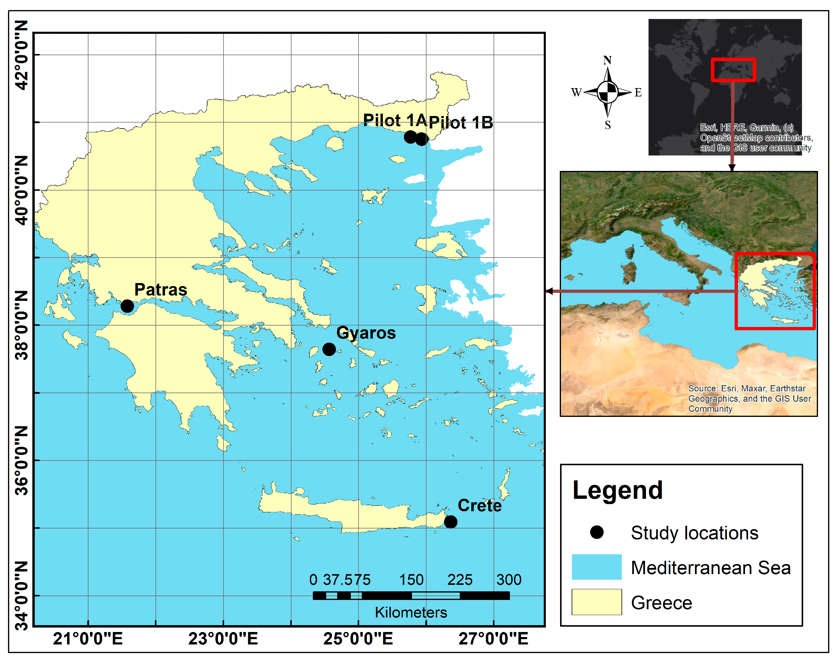
2.1. Study Area and Data Source

One of the most energetic areas in the Greek seas regarding wind energy (>10 m/s/year) is located in the southern parts of the Aegean Sea, and specifically off the eastern parts of Crete Island. The particular area (polygon) is located near the eastern coast of Crete Island, with central coordinates 35.09° N–26.36° E, and a total size of 118 km². It is well-suited for floating wind installations. Similarly, high wind speeds are observed in the central Aegean, specifically in the offshore areas northwest of Gyaros Island, where the polygon Gyaros, with central coordinates 37.64° N–24.57° E, is a potential location for a floating installation. For fixed-bottom development, there are two sites considered in this study. The polygon in the Gulf of Patras, with central coordinates 38.28° N–21.58° E, and a total size of 138.84 km², is located in a less windy area (~7 m/s/year). The Pilot area is located near the southern coast of Alexandroupolis in the northern part of the Aegean Sea, with mean annual wind speeds of up to 6–7 m/s, including two potential polygons (Pilot 1A and 1B, with central coordinates 40.78° N–25.77° E and 40.75° N–25.93° E, respectively) with a total size of 219.42 km² (see Figure 1). For a detailed analysis of wind speeds over the Greek seas, see [52].

In this research, we utilized the ERA5 reanalysis data from the European Centre for Medium-Range Weather Forecasts [53,54]. ERA5 provides hourly averaged estimates of various ocean wave, atmospheric, and land-surface parameters, thereby providing a comprehensive overview of the Earth’s climate and weather over several decades, with data dating back to 1940. The ERA5 dataset has been globally evaluated, and it has yielded uninterrupted and reliable atmospheric datasets across both space and time [55,56,57]. It is frequently employed to evaluate wind and wave climatology, as well as to conduct long-term analyses of climate change effects on wind and wave climates, [3,49,58,59].

The wind speed’s horizontal and vertical components, $u_{100}$ and $v_{100}$ respectively, at a 100 m height above sea level were extracted from ERA5 for each study location. The resultant wind speed $w_{100}$ was then calculated from the $u_{100}$ and $v_{100}$ components, i.e., $w_{100}=\sqrt{u_{100}+v_{100}}$. The data spans a period of 39 years (1985–2003).

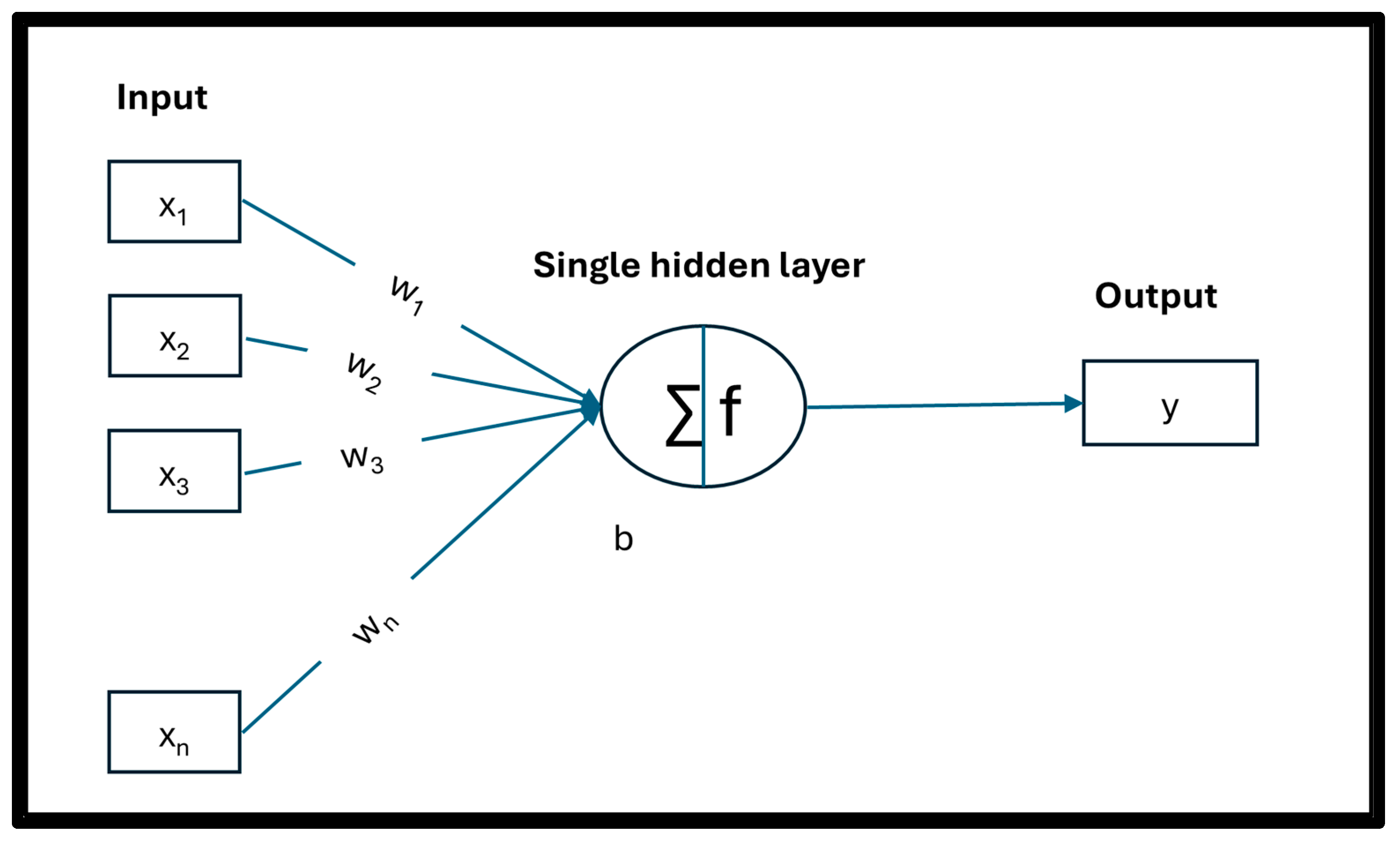
2.2. Feedforward Neural Network

A feedforward neural network (FFN) is a form of a multilayered perceptron that has been reported to be suitable for the modeling, calibration, and prediction of ocean hydrological parameters [60,61,62,63,64]. Its architecture comprises three layers: input, hidden, and output layers (see Figure 2). The number of hidden layers and neurons per layer determines a model’s capacity to learn complex patterns, with more layers and neurons potentially enabling the model to capture more intricate relationships, but also increasing the risk of overfitting. Each input is multiplied by the associated weight, and the sum of all the weighted terms and bias is passed through an activation function, whose purpose is to capture the complexity and nonlinearity of the series. The weight coefficient matrix and the bias are determined by repeated training of the network.

$$y\left(x\right)=f(\sum _{i=1}^n{x}_i{w}_i+b),$$

(1)

where $f$ is the activation function; $b$ is the bias; and $x_i\mathrm{a}\mathrm{n}\mathrm{d}{w}_i,\mathrm{w}\mathrm{i}\mathrm{t}\mathrm{h}i=\mathrm{1,2},\dots ,n,$ are the normalized (standardized) inputs and weights, respectively.

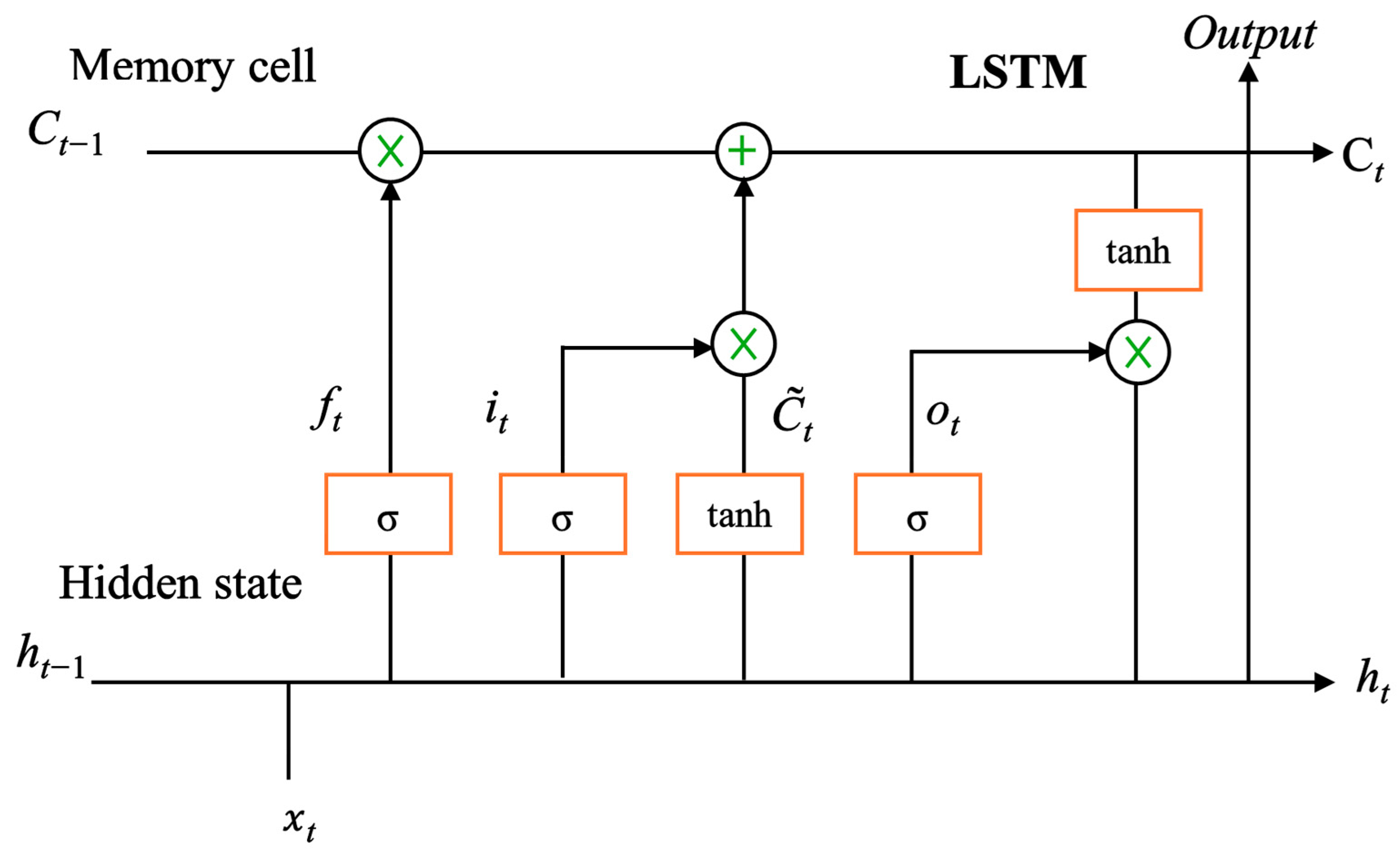
2.3. Long Short-Term Memory Network

An LSTM is a special type of recurrent neural network designed to effectively model long-term dependencies within time series data [37]. Hochreiter and Schmidhuber [65] first introduced the LSTM method, which builds on the fundamental principles of a simple RNN. Unlike a simple RNN, which suffers from the vanishing gradient problem, LSTM networks are designed to address this challenge by incorporating memory cells and gate mechanisms that enable the network to retain and discard information from prior time steps. An LSTM consists of an input gate, forget gate, and output gate. Figure 3 illustrates the structure of a unit cell of LSTM data flow.

The gates serve distinct roles in regulating the flow of information through the network, as they allow some information to pass through while restricting some information. The forget gate determines which information from the previous time step’s hidden state is important to retain. The input gate regulates the addition of new information from the current time step to the cell state, and the output gate determines which components of the cell state should be utilized to generate the output for the current time step.

Formally, the LSTM update equations are provided as follows:

$$f_t={\sigma (W}_f.\left[h_{t-1},x_t\right]+b_f),$$

(2)

$$i_t={\sigma (W}_i.\left[h_{t-1},x_t\right]+b_i),$$

(3)

$$o_t={\sigma (W}_o.\left[h_{t-1},x_t\right]+b_o),$$

(4)

$$C_t=f_t.C_{t-1}+i_t.{\tilde{C}}_t,$$

(5)

$${\tilde{C}}_t={\mathrm{t}\mathrm{a}\mathrm{n}\mathrm{h}(W}_c.\left[h_{t-1},x_t\right]+b_c),$$

(6)

$$h_t=o_t\ast \tanh \left(C_t\right),$$

(7)

where $f_t$, $i_t$, and $o_t$ are the forget gate, input gate, and output gate, respectively; $x_t$ is the input sequence at time $t$; and $h_{t-1}$ is the previous output of the LSTM cells at time $t-1$. ${\tilde{C}}_t$ is the candidate or temporary value at time $t$. $C_t$ is the memory cell state, and $h_t$ is the hidden state. $W_f,W_i,{\mathrm{a}\mathrm{n}\mathrm{d}W}_o$ are the weight matrices of the forget, input, and output gates, respectively, while $b_f,b_i,{\mathrm{a}\mathrm{n}\mathrm{d}b}_o$ are the corresponding biases. $\sigma \left(·\right)$ is the sigmoid activation function, $\mathrm{t}\mathrm{a}\mathrm{n}\mathrm{h}\left(·\right)$ is the hyperbolic tangent activation function, and ‘*’ is the Hadamard product or element-wise product.

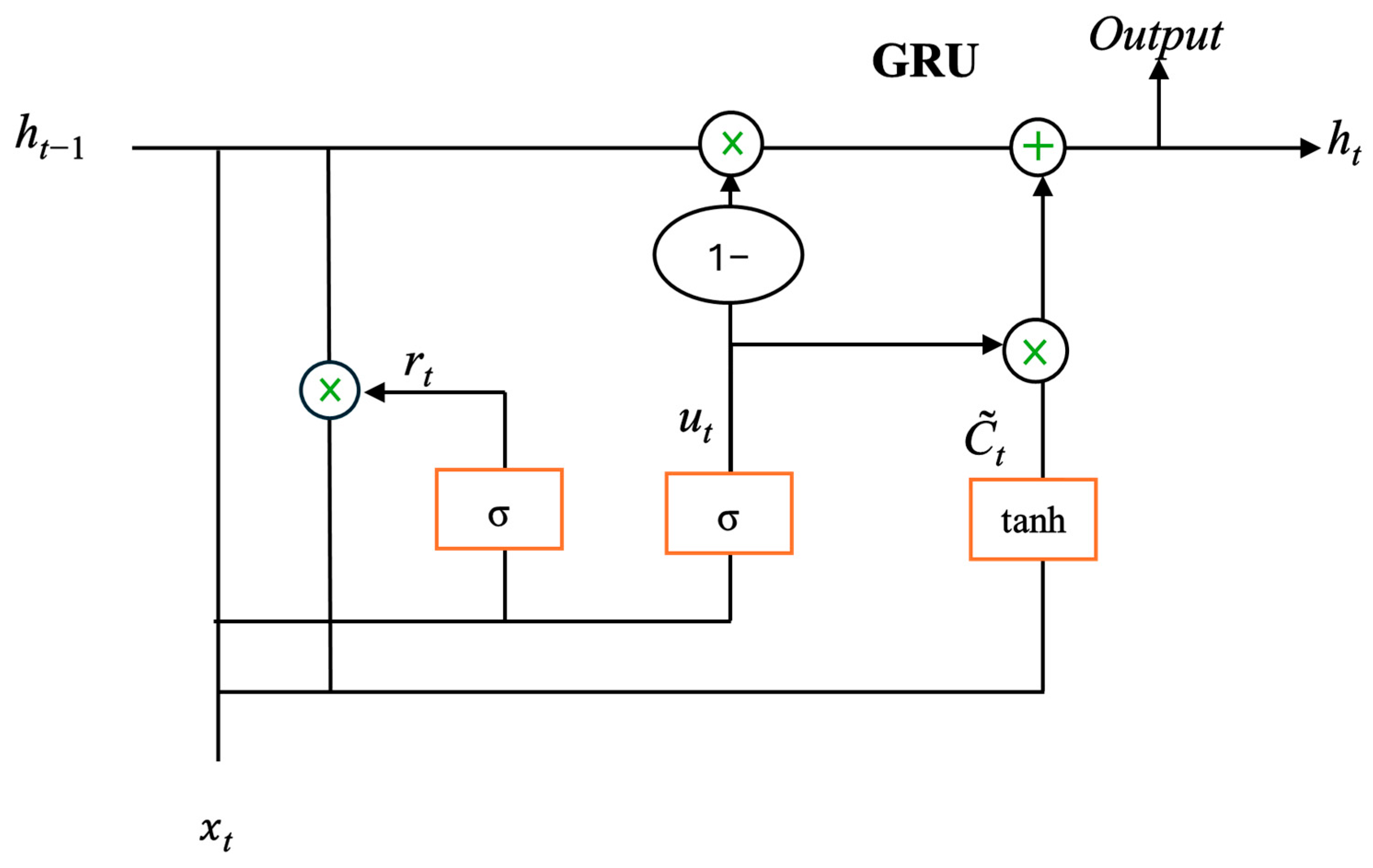
2.4. Gated Recurrent Unit Network

Another important element of the proposed hybrid model is the GRU, which is a recurrent neural network architecture that is analogous to the LSTM network but with a simpler structure (Figure 4). A GRU also uses gate mechanisms to control the flow of information, but it has fewer parameters than an LSTM, making it computationally more efficient. Unlike an LSTM, which has three gates, a GRU utilizes only two gate mechanisms—the reset and update gates. In a GRU, both the long and the short term are combined into a single hidden state. The reset gate enables the hidden state to discard information deemed irrelevant, while the update gate retains and regulates the combination of past and current state data to generate the current output.

The hidden state $h_t$ (Equation (8)) is a combination of the update gate and candidate value ${\tilde{C}}_t$. The equation for the candidate value (Equation (10)) is very similar to the equation of activation in a simple RNN. The update gate $u_t$ (Equation (9)) is designed in such a way that it takes either 0 or 1 as its value. The equation of the hidden state has two parts: $u_t$ and $1-u_t$. Since the update gate $u_t$ can take either only zero or one as its value, then only one of these parts exerts its effect when calculating the $h_t$. If the update gate $u_t$ is close to zero, then this value will be nullified, and the hidden state $h_t$ will be equal to the previous hidden state $h_{t-1}$. Therefore, the hidden state will not be updated at this time step, since it is simply assigned the value from the previous time step. However, if the value of $u_t$ is close to one, then the previous value of the hidden state $h_{t-1}$ will be nullified and thus it will add the candidate value into its memory state. During training, the values of the weight ($W)$ matrix determine what information will be forgotten or retained by the update gate. The model will learn to adjust the weight matrix in a way that allows it to discern which information is relevant and which is not, thereby improving its understanding. The value of the update gate in a GRU model can vary based on the input wind speed at each time step, allowing the model to adaptively capture the relevant information. The reset gate equation $r_t$ (Equation (11)) is similar in structure to the equation of the update gate, but it uses different weight matrices to control the flow of information from the previous hidden state. The reset gate is present in the equation of the candidate value, where it controls how much of the previous hidden state is used to compute the current candidate’s hidden state. This enables the model to strategically retain or discard information from the preceding time step, enabling it to adaptively capture the relevant information for forecasting.

The GRU update equations are as follows:

$$h_t=u_t\ast {\tilde{C}}_t+\left(1-u_t\right)\ast h_{t-1},$$

(8)

$$u_t=\sigma (W_u\left[h_{t-1},x_t\right]+b_u),$$

(9)

$${\tilde{C}}_t=\mathrm{t}\mathrm{a}\mathrm{n}\mathrm{h}(W_c\left[r_t\ast h_{t-1},x_t\right]+b_c),$$

(10)

$$r_t=\sigma \left(W_r\left[h_{t-1},x_t\right]+b_r\right),$$

(11)

where $u_t$ is the update gate, $r_t$ is the reset gate, and $h_t$ is the hidden state. $b_u$ and $b_r$ are the bias vectors of the update and reset gate, respectively. $W_u,W_r,{\mathrm{a}\mathrm{n}\mathrm{d}W}_c$, are the weight matrix of the update gate, reset gate, and candidate value respectively.

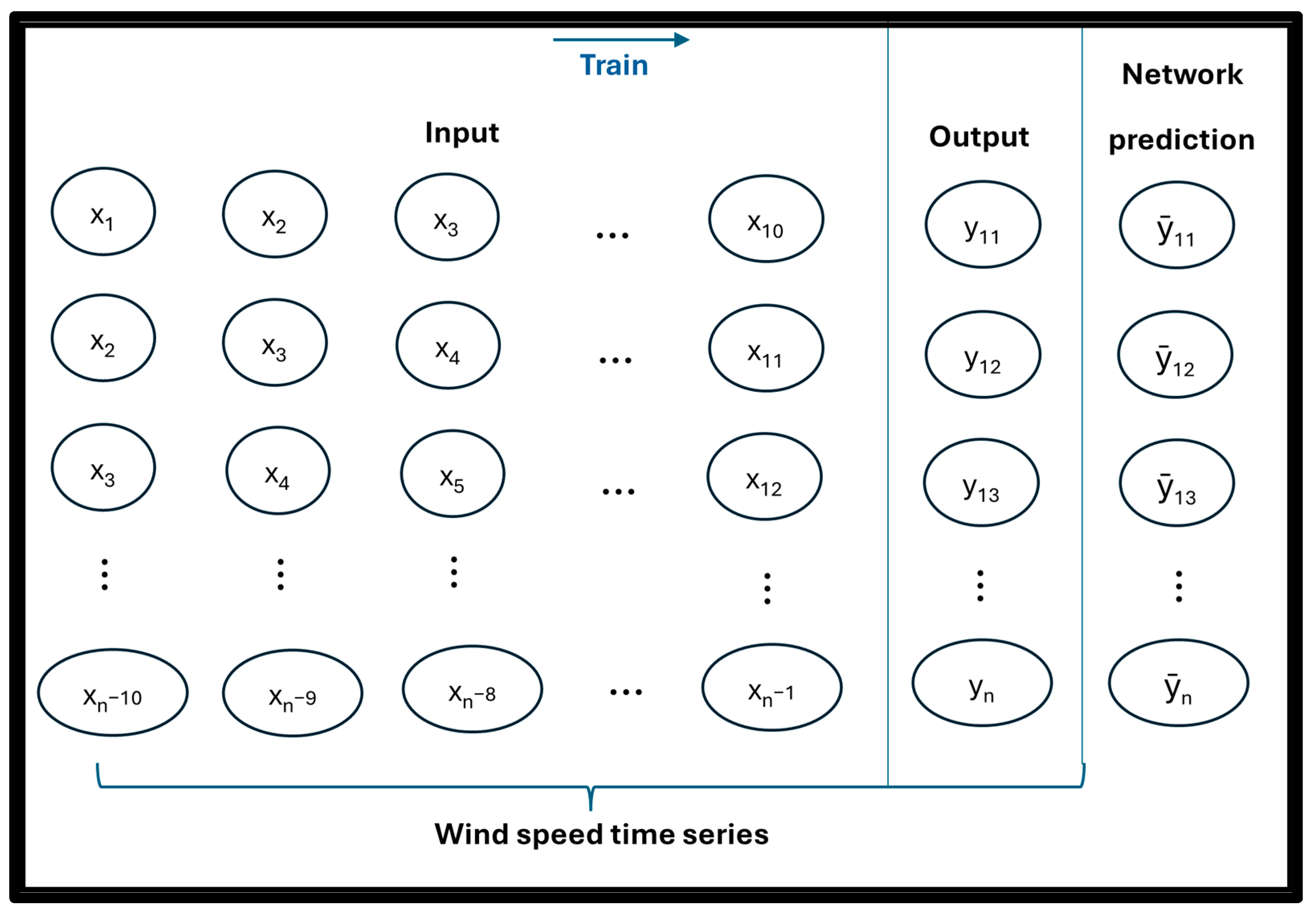
2.5. Experimental Approach

Let $x=[x_1,x_2,\dots ,x_t]$ be the time series of wind speed measurements to be forecasted. The datasets were standardized (normalized) and then partitioned into training and testing subsets in the proportions of 80% and 20%, respectively, prior to model training. Both the training and the test series were reshaped into input and output using the sliding window approach (Figure 5).

The networks were designed to predict the next time step using the previous ten steps for each row of the input data fed into the networks. For each standalone LSTM and GRU, the model was trained using only the training series with 128 neurons in the hidden layer, then with a dropout of 25% to prevent overfitting. Finally, the sequence was fed into a fully connected layer to generate the final output. For the hybrid model, both the LSTM and GRU layers were stacked together and then passed through a dropout layer. Another LSTM layer was used to finally capture the temporal patterns, and the sequence was fed into a fully connected layer to generate the final output. The initial LSTM layer received feedback from its previous time step and captured certain patterns, which served as the input into the GRU. To avoid overfitting, the dropout layer excluded 25% of the neurons. After several experimental setups, the neurons in each layer of LSTM, GRU, and LSTM were set at 128, 64, and 32, respectively. This hierarchical structure facilitates the network’s ability to complexly represent the wind speed time series data and capture information at varying scales. The FFN was trained with Bayesian regularization, i.e., a backpropagation algorithm that optimizes the weights and biases through minimizing a combination of the squared errors and weights to produce a network that generalizes well by matching the input datasets to the output, while it also prevents overfitting. The number of neurons in the single hidden layer was 20. The validation fail check was set to 30, and this stopped the training once it reached the best performance.

The standalone FFN, LSTM, and GRU models were used to facilitate a comparison between each model and the hybrid one. The models were trained using 80% of the ERA5 historical wind speed data from the Greek seas for each of the study locations, and their performances were evaluated using various error metrics, such as the $RMSE$, mean absolute error ($MAE$), and mean absolute percentage error ($MAPE$). Graphical visualizations were also employed to supplement the quantitative error metrics and provide visual representations of the models’ effectiveness. The mean squared error ($MSE$) was selected as the loss function. The rest of the hyperparameters are shown in

Table 1. Some hyperparameters used in training of all examined networks.

	FFN	LSTM	GRU	Hybrid
Epoch	1000	100	100	100
Learning rate	0.001	0.001	0.001	0.001
Dropout	-	0.25	0.25	0.25
Minibatch	-	512	512	512
Optimizer	Bayesian	Adam (1)	Adam	Adam
Weight optimizer	-	Glorot	Glorot	Glorot

¹ Adaptive moment estimation: combines the momentum and root mean square propagation techniques.

.

2.6. Network Performance

The performance of all the networks using the trained models was assessed. These models were quantitatively assessed using four statistical metrics, i.e., the $MAE$, $MAPE$, $RMSE$, and the coefficient of determination $R^2,$ to comprehensively evaluate the performance of each model. These metrics are defined as follows:

$$MAE={\displaystyle \frac{1}{N}}\sum _{t=1}^N|x\left(t\right)-\widehat{y}\left(t\right)|,$$

(12)

$$MAPE={\displaystyle \frac{1}{N}}\sum _{t=1}^N|{\displaystyle \frac{x\left(t\right)-\widehat{y}\left(t\right)}{y\left(t\right)}}|.100,$$

(13)

$$RMSE=\sqrt{{\displaystyle \frac{1}{N}}\sum _{t=1}^N[{x\left(t\right)-\widehat{y}\left(t\right)]}^2},$$

(14)

$$R^2=1-{\displaystyle \frac{\sum _{t=1}^N{\left[x\left(t\right)-\widehat{y}\left(t\right)\right]}^2}{\sum _{t=1}^N{\left[x\left(t\right)-\overline{x}\right]}^2}},$$

(15)

where $\widehat{y}\left(t\right)$ is the predicted wind speed by the network, $x\left(t\right)$ is the actual wind speed, $\overline{x}$ is the sample mean value, and $N$ is the number of samples of the time series.

3. Results and Discussion

To mitigate the limitations of conventional statistical models and to capture the complex, nonlinear, and dynamic nature of the wind patterns in the Greek seas, we examined standalone and hybrid artificial neural network models for short-term wind speed forecasting. Each neural network architecture already described was tested using the potential OWFODAs in the Greek seas, i.e., Crete, Gyaros, Patras, Pilot 1A, and Pilot 1B. The remaining 20% (testing) of the whole dataset was used to evaluate the accuracy of the trained models.

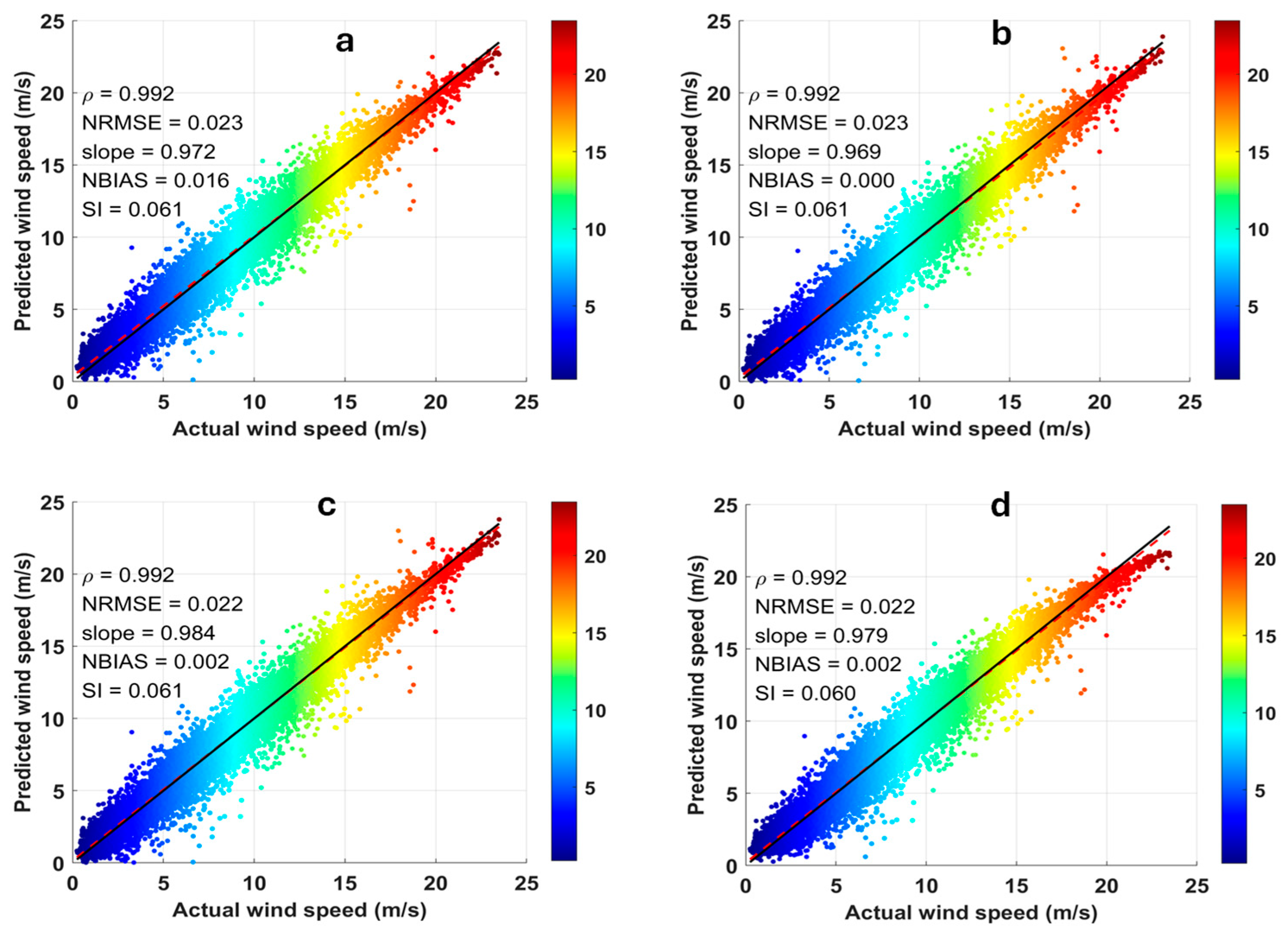
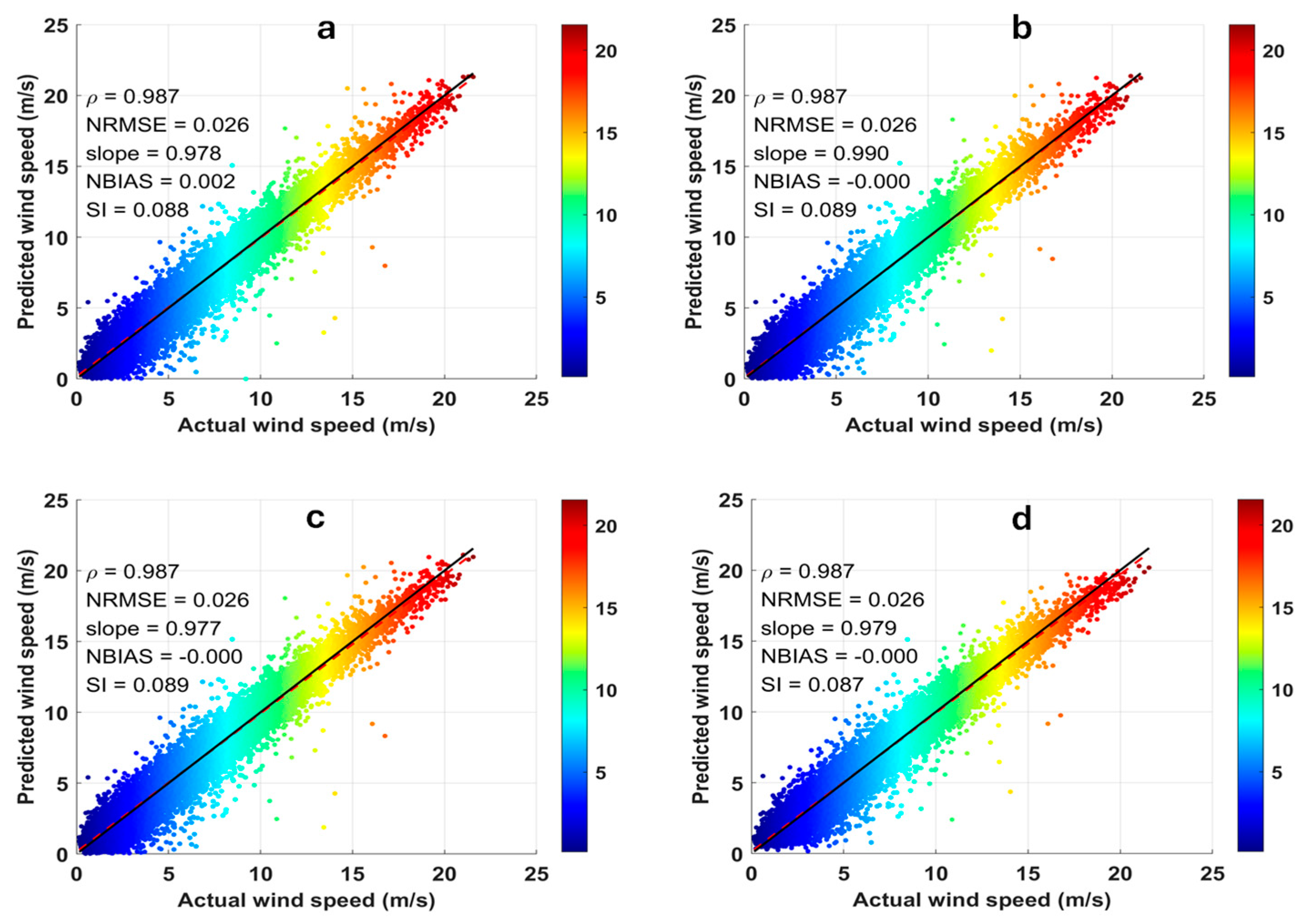
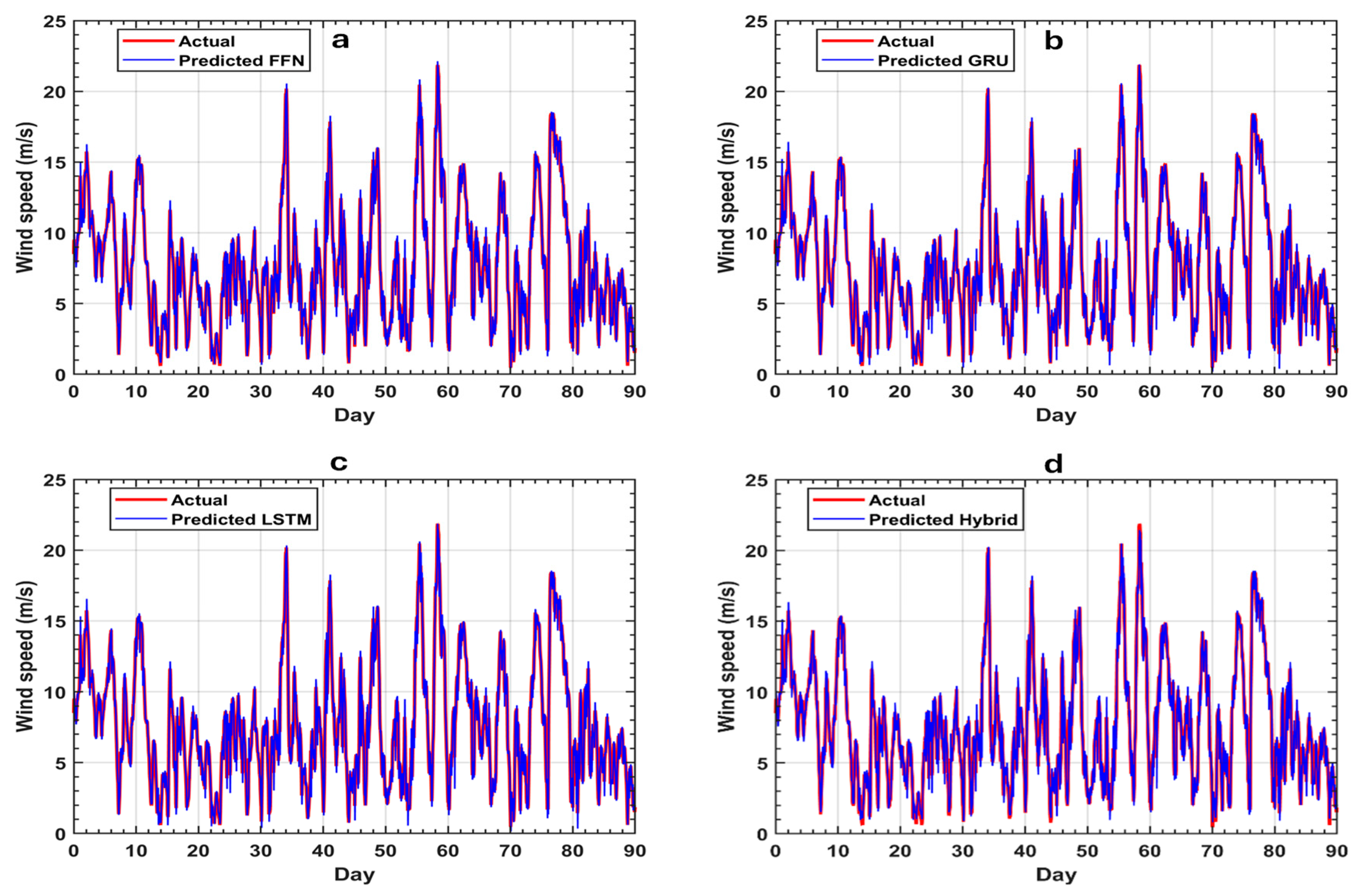
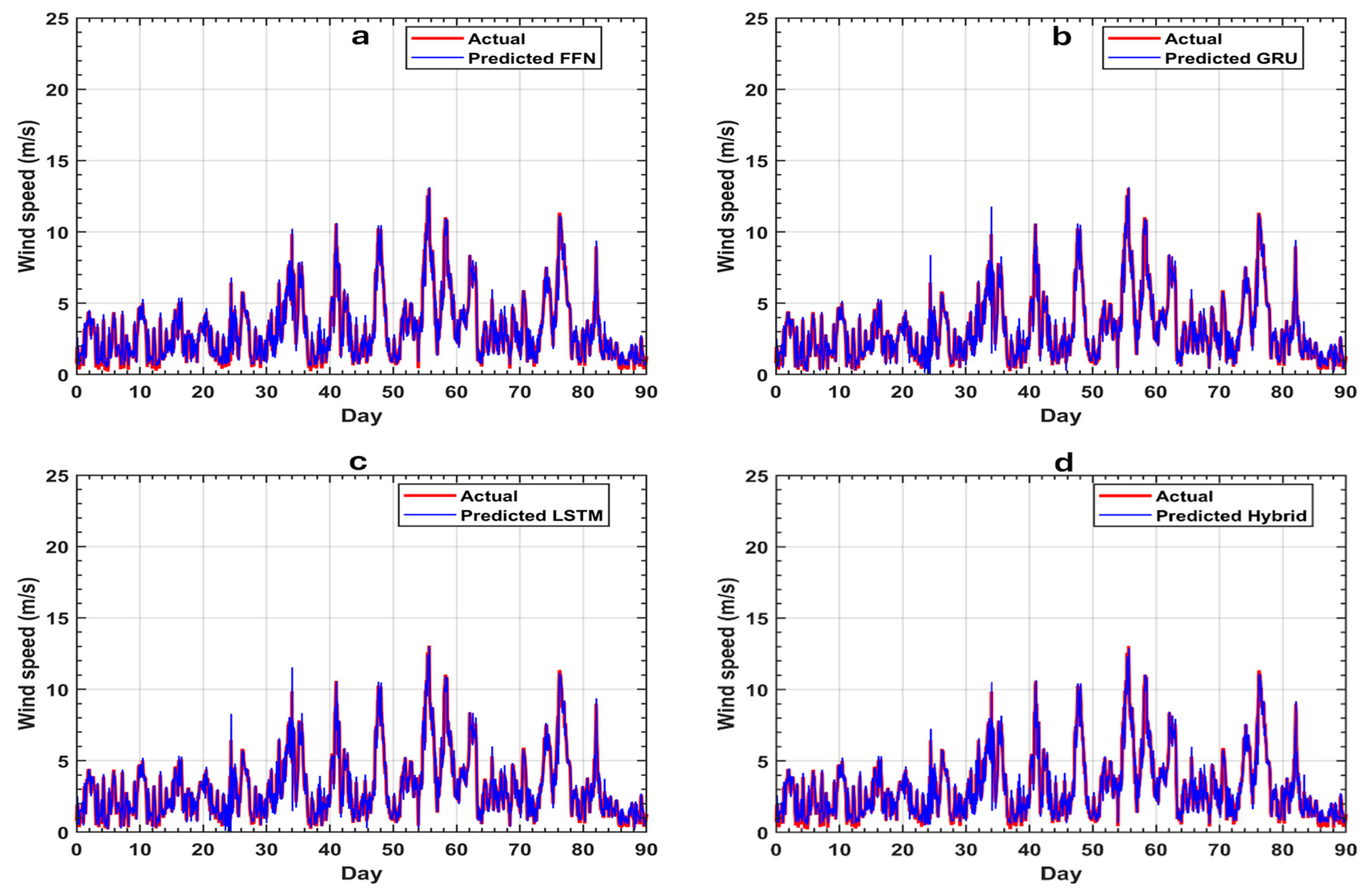
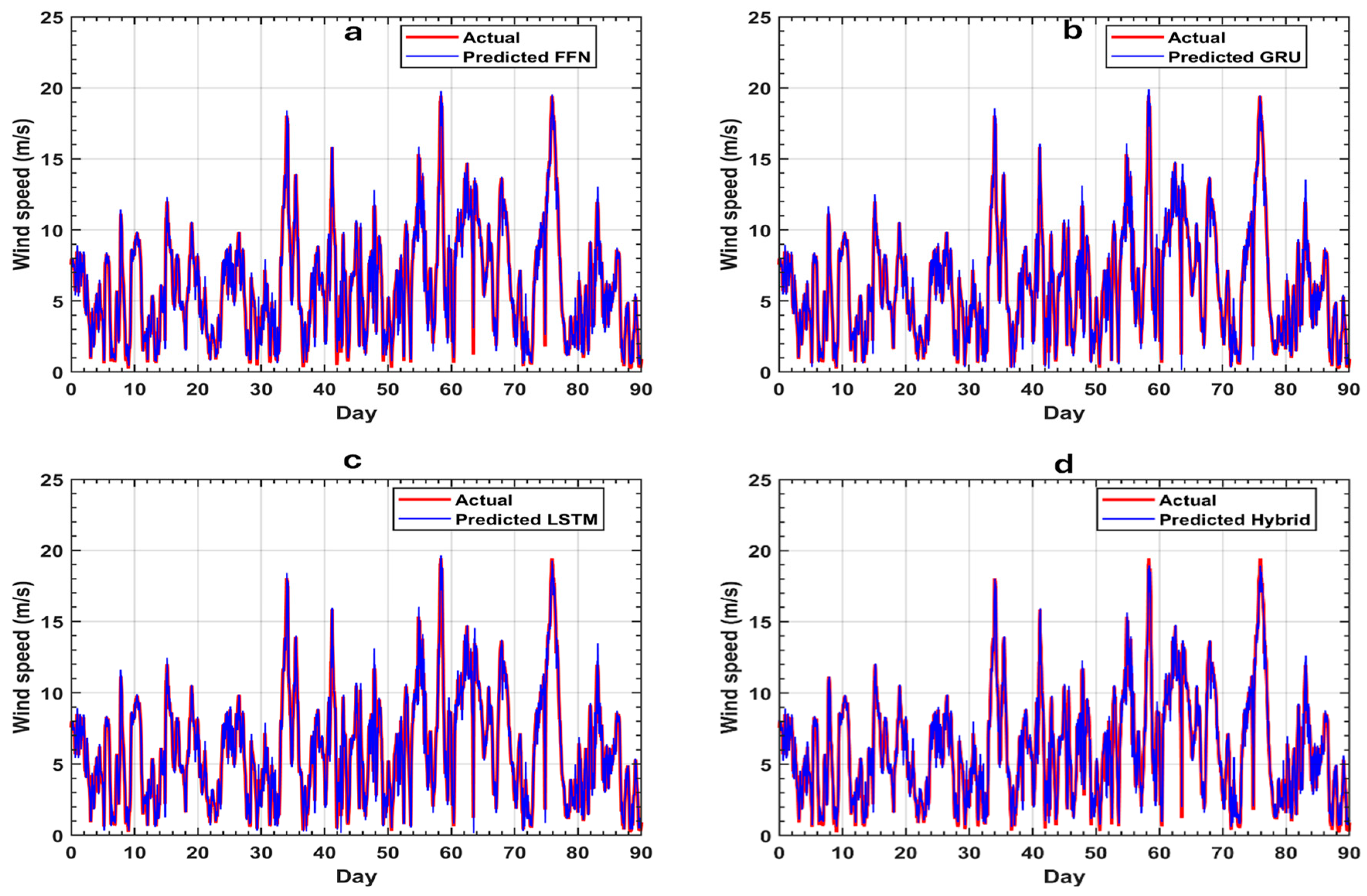
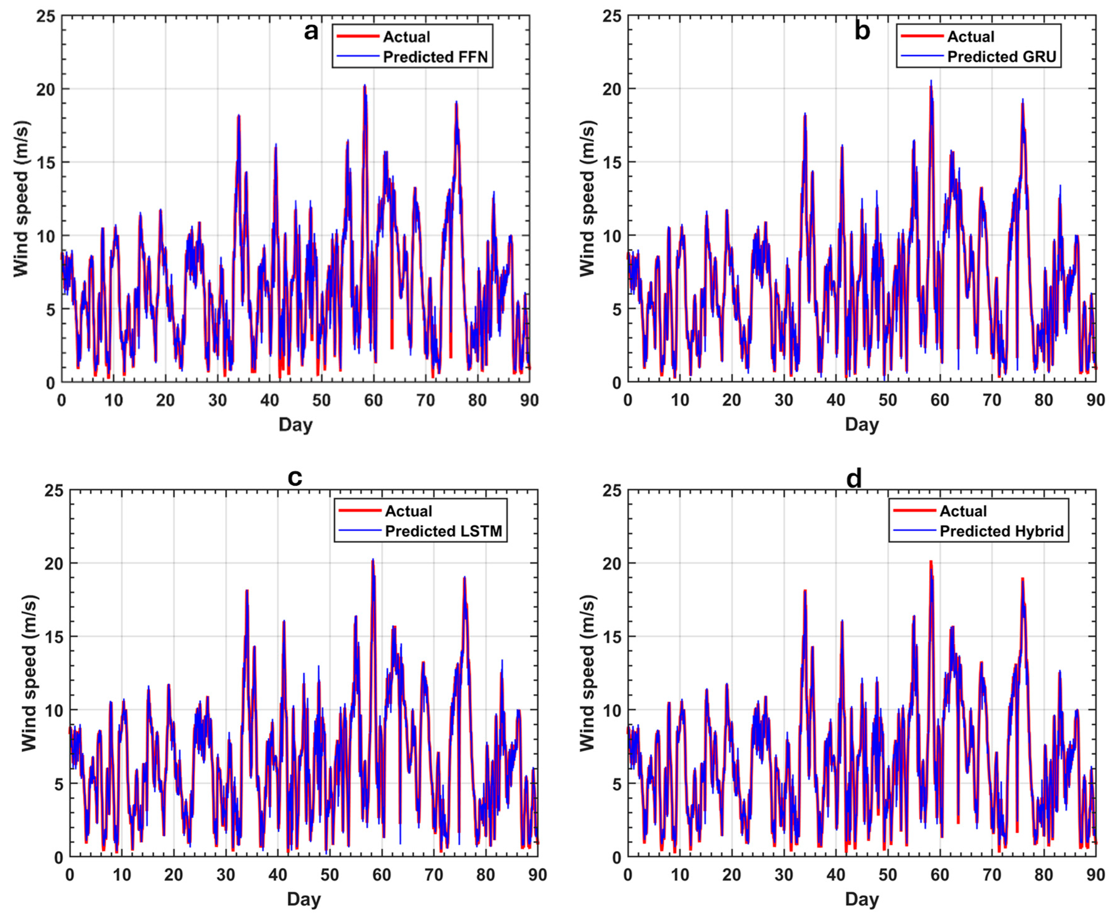
3.1. Network Prediction Results

Figure 6, Figure 7, Figure 8, Figure 9 and Figure 10 present scatter plots of the predicted wind speeds from each network against the actual measurements for Crete, Gyaros, Patras, Pilot 1A, and Pilot 1B, respectively. The red dashed lines are the regression lines and the black lines are the lines passing from the origin (0,0).

For Crete, the Pearson correlation coefficient, $\rho ,$ is 0.99 across all the methods, indicating a very high correlation, with only a negligible percentage of predictions diverging from the actual wind speed values. While the feedforward neural network exhibited a very small normalized bias ($NBIAS$) of 0.02, all the other methods demonstrated an $NBIAS$ of 0. The normalized root mean square error ($NRMSE$) was 0.02 for all the models. Additionally, the scatter index ($SI$) was consistently 0.06 across the networks. The empirical findings suggest that the hybrid model consistently outperformed the individual FFN, GRU, and LSTM networks, as evidenced by its having the lowest $RMSE$ values (0.5162 m/s) and $R^2=0.9850$ (see also

Table 2. Results of the performance of different networks at each study location.

	Networks	$\mathit{R}\mathit{M}\mathit{S}\mathit{E}$ (m/s)	Bias (m/s)	$\mathit{M}\mathit{A}\mathit{E}$ (m/s)	$\mathit{M}\mathit{A}\mathit{P}\mathit{E}$ (%)	${\mathit{R}}^2$
Crete	FFN	0.5407	0.1342	0.3647	6.9700	0.9835
	GRU	0.5272	0.0025	0.3482	6.3335	0.9843
	LSTM	0.5218	0.0158	0.3374	6.0118	0.9847
	Hybrid	0.5162 (2)	0.0156	0.3364	6.1220	0.9850
Gyaros	FFN	0.5922	0.0374	0.3892	7.5320	0.9815
	GRU	0.5907	0.0010	0.3889	7.4216	0.9816
	LSTM	0.5904	−0.0178	0.3890	7.3971	0.9816
	Hybrid	0.5890	0.0019	0.3860	7.3415	0.9817
Patras	FFN	0.5059	0.0229	0.3594	18.6159	0.9414
	GRU	0.5085	−0.0074	0.3602	18.2314	0.9408
	LSTM	0.5061	−0.0007	0.3597	18.3491	0.9413
	Hybrid	0.4983	−0.0274	0.3508	17.4819	0.9431
Pilot 1A	FFN	0.5894	−0.0152	0.4027	11.6456	0.9714
	GRU	0.5925	−0.0147	0.4060	11.8742	0.9711
	LSTM	0.5918	−0.0144	0.4023	11.6145	0.9712
	Hybrid	0.5766	0.0142	0.3964	11.7795	0.9727
Pilot 1B	FFN	0.5627	0.0136	0.3838	9.8234	0.9736
	GRU	0.5658	−0.0001	0.3834	9.5777	0.9733
	LSTM	0.5636	−0.0018	0.3839	9.8400	0.9735
	Hybrid	0.5529	−0.0001	0.3795	9.7007	0.9745

² Boldface denotes the best prediction result.

).

For Gyaros, Patras, Pilot 1A, and Pilot 1B, the values of $\rho$ ranged from 0.97 to 0.99, with all the models achieving 0.99 at three out of the four locations, except at Patras, where the value was 0.97 for all the models. The $SI$ ranged from 0.07 to 0.16, with the lowest for Crete and the highest for Patras.

The residuals between the network predictions and the actual wind speed measurements are depicted in Figure 11, Figure 12, Figure 13, Figure 14 and Figure 15. For Crete, most of the errors, accounting for 94% of the total, fell within the range of ±1 m/s, while 99% were within ±2 m/s. The percentages of errors greater than 1 m/s were 0.059%, 0.056%, 0.056%, and 0.055% for the FFN, GRU, LSTM, and the hybrid, respectively. This indicates that the networks exhibited a strong ability to accurately predict the wind speeds, with only a negligible percentage of outliers. The negligible remaining percentage can be attributed to the very large dataset used to evaluate the networks’ precision, which helped to provide a comprehensive assessment of the model’s performance. Nevertheless, all the networks demonstrated a substantial capacity to learn patterns from decades of historical wind speed data, showcasing their robustness and reliability for wind speed forecasting. For the rest of the examined areas, the errors ranged between ±4 m/s, with the largest percentage of errors in the range of ±1 m/s.

Table 2 summarizes the evaluation results for the four networks for all the locations. The best prediction results for each metric for each location are shown in boldface. The hybrid model had the lowest value of the $RMSE$ at all the locations ($RMSE=0.4983\mathrm{m}/\mathrm{s}$ in Patras). Both the hybrid and the GRU had the lowest bias of −0.0001. The hybrid had the lowest $MAE$ at all the locations, with an $MAE=0.3364\mathrm{m}/\mathrm{s}$ for Crete. The LSTM had the lowest value of the $MAPE$, with a value of 6.0118, and the highest value of the said metric at Patras ($MAPE=18.616\mathrm{\%}$). The hybrid had the highest coefficient of determination $R^2$ at each location, with the highest value of 0.9850 for Crete. As regards the overall prediction effect, the $RMSE$, $MAE,$ and $R^2$ of the hybrid network were less than those of the other network predictions for all the examined locations, while for Pilot 1B the hybrid network provided the optimal values for all the examined metrics.

Moreover, panels a in Figure 16, Figure 17, Figure 18, Figure 19 and Figure 20 present an hourly comparison between the actual wind speed data and the predicted outputs of all the different neural network models, and panels b show the residuals (errors) of each network’s predictions for Crete Island, Gyaros, Patras, Pilot 1A, and Pilot 1B, respectively. The time series plot spans 336 h (14 days), with the wind speed values ranging from 0 to 20 m/s, with the lowest maximum value of 14 m/s for Patras. All the models demonstrated strong predictive performance, closely tracking the actual wind speed trends. The hybrid model, shown in magenta, consistently aligned with the actual data, particularly during high-variability and peak events, suggesting its superior temporal generalization. The LSTM (red) and GRU (green) models also achieved high fidelity, effectively capturing both rapid transitions and steady-state behaviors. The FFN (black), while slightly less responsive during sharp fluctuations, still maintained a competitive performance, especially for smoother segments of the time series. Furthermore, regarding the error dynamics shown in the b panels of the above-mentioned figures, it can be seen that the feedforward neural network (FFN) exhibited higher variability, with its error magnitudes occasionally exceeding ±2.0 m/s. In contrast, the hybrid model maintained a more stable error distribution, generally confined within ±1 m/s. Both the LSTM and GRU models also showed improved error consistency compared to the FFN, though they exhibited slightly higher fluctuations than the hybrid approach. This indicates that recurrent-based models (LSTM and GRU) are more capable of handling temporal dependencies than the static FFN architecture, while the hybrid model achieves a balance between capturing long-term patterns and minimizing error propagation.

Overall, among the models compared, the hybrid approach showed the closest approximation to the actual values throughout the entire duration. This suggests that the integration of multiple architectures can potentially leverage the strengths of individual networks, thereby enhancing the overall prediction accuracy. These findings underscore the effectiveness of deep learning techniques, particularly hybridized structures, for capturing the complex dynamics of wind speed variability.

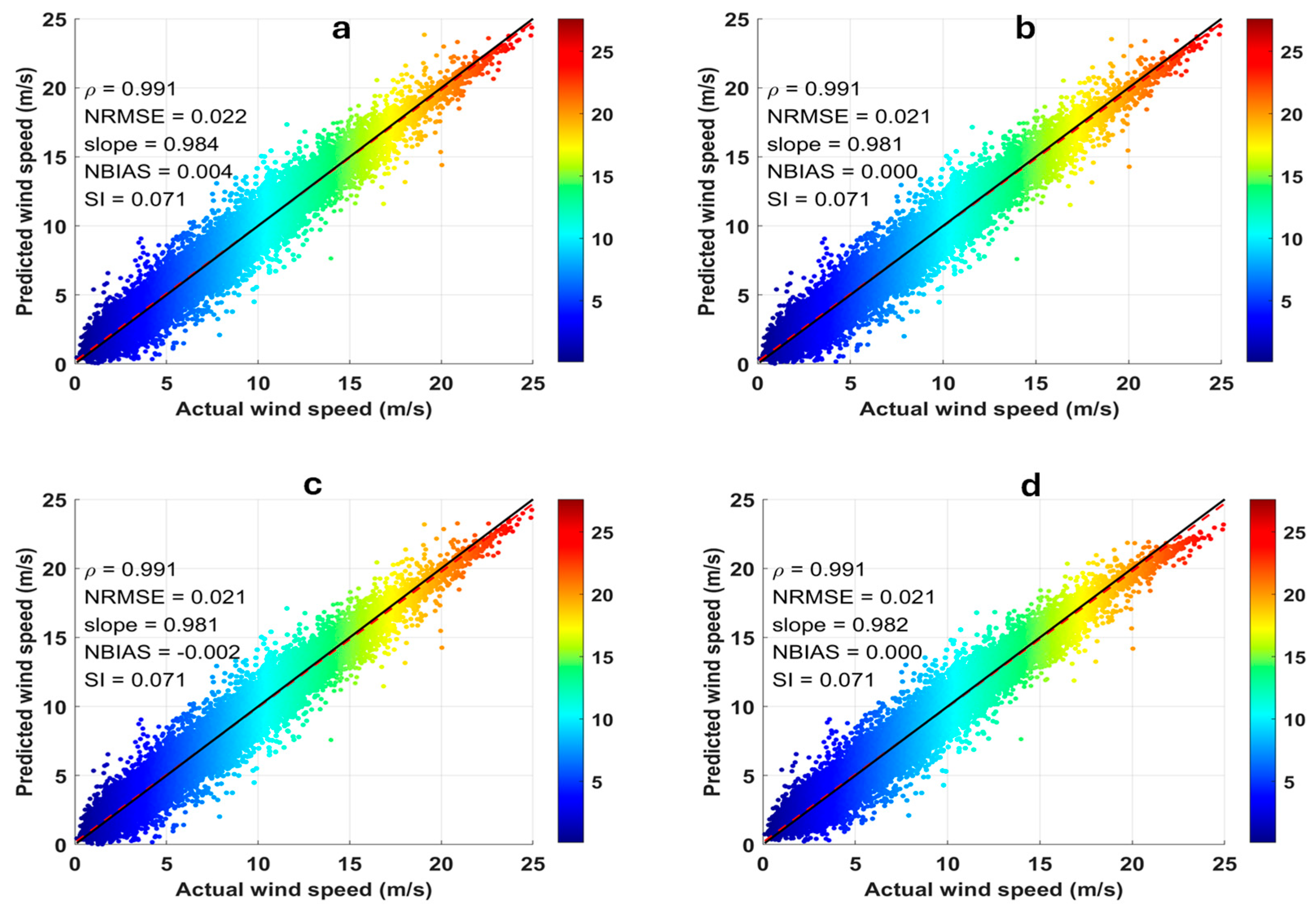
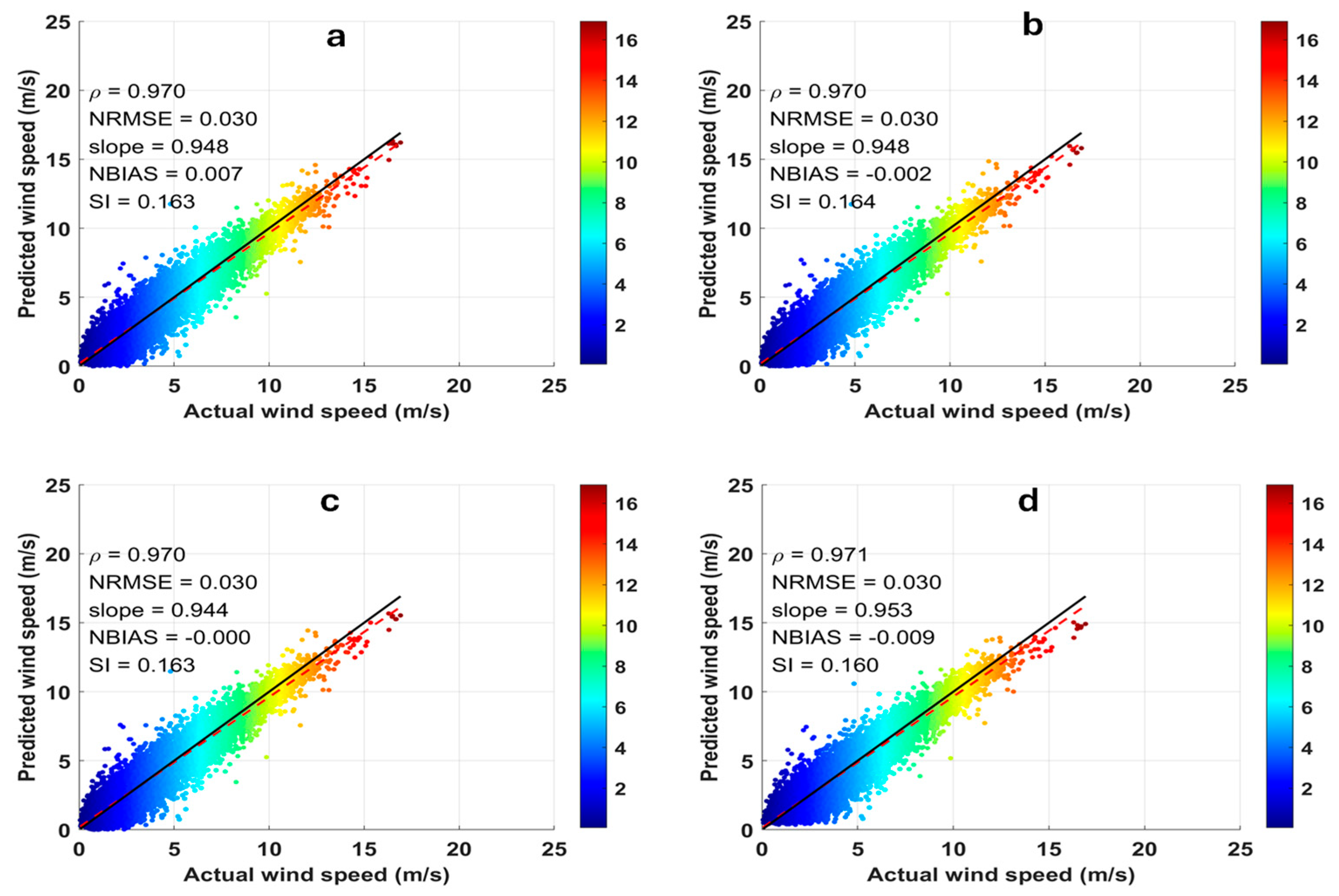
3.2. Network Prediction Results with Fresh Data

To evaluate the generalization capability of the models beyond the training window, a separate test dataset spanning approximately 90 days was used. Figure 21, Figure 22, Figure 23, Figure 24 and Figure 25 show the time series of all the network predictions and the actual wind speeds for October to December 2023 at Crete, Gyaros, Patras, Pilot 1A, and Pilot 1B, respectively. Visually, all the models demonstrated a strong ability to follow the underlying wind speed patterns across an extended time horizon, including rapid fluctuations and prolonged calm periods. Each network had a very good prediction of the wind speed, with only a very slight underestimation of the wind speeds, with a value less than 1.0 m/s. However, let us remember that ERA5 underestimates low wind speeds [55]. Overall, and despite the increased complexity of and variability in the test data, the predicted series closely follows the actual measurements, with minimal phase shifts or amplitude damping.

3.3. Discussion

The results of the several experiments show that the proposed hybrid model outperformed the baseline models in terms of forecasting accuracy, as measured by the statistical metrics (Table 2). The hybrid model’s superior performance stems from its capacity to capture both the long-term trends and short-term variations in the wind speed data. The hybrid model was able to leverage the strengths of both the LSTM and GRU networks to provide more accurate and reliable wind speed forecasts than the individual models. Although the hybrid model requires slightly more processing time than the standalone models, the improvement in forecasting accuracy justifies the additional computational cost. In general, across all the scenarios, from short-term fluctuations to the model’s residuals to its long-term prediction, the hybrid model consistently demonstrated superior performance. Its ability to retain low error margins and high statistical scores makes it a viable candidate for deployment in real-world wind forecasting systems, particularly where both precision and stability are critical.

The network architectures demonstrate the capability to forecast wind speed. However, accurate wind speed forecasts do not depend solely on the architecture, but also on the accuracy of the wind speed data, as a network’s precision capability is a function of the data used for training. The ERA5 data used for the case studies has been reported to underestimate and overestimate wind and wave climate parameters in enclosed seas [66]. The scarcity and discontinuity of the observational wind speed, due to many factors, made it difficult to use in this study. However, available observational data can be used to calibrate the publicly available ERA5. Testing the architecture on the calibrated wind speed could improve wind speed forecasting, the importance of which cannot be overemphasized.

4. Conclusions

We examined different machine learning algorithms suitable for wind speed forecasting. Five potential hotspot areas of high wind power potential were used as case studies for testing the capacity of the algorithms to predict future wind speeds, which are vital for many applications. Our results highlight the very good performance of the networks at all the tested sites using the ERA5 reanalysis historical wind speed dataset. The hybrid model achieved the lowest root mean square errors across all the sites—0.52 m/s (Crete), 0.59 m/s (Gyaros), 0.49 m/s (Patras), 0.58 m/s (Pilot 1A), and 0.55 m/s (Pilot 1B)—and an average coefficient of determination ($R^2$) of 97%. The hybrid model produced the best prediction results with the lowest values of the statistical metrics used for the estimation of the trained models’ performance. Moreover, the performance of the hybrid model was also very good at high wind speeds, i.e., above 15 m/s, while at the very low wind speeds, i.e., below 2 m/s, there was a slight overestimation. A future task will be to improve the accuracy of the ERA5 parameters by recalibrating them with the available observational data. Then the networks will be tested with the calibrated data to improve the wind speed predictions. Additionally, other parameters that could influence the wind speed will be considered and used to train the networks to enhance their understanding of the patterns and to determine how they can be incorporated into the networks to provide even more accurate wind speed predictions.

References

1. Contestabile, P.; Di Lauro, E.; Galli, P.; Corselli, C.; Vicinanza, D. Offshore Wind and Wave Energy Assessment around Malè and Magoodhoo Island (Maldives). Sustainability 2017, 9, 613. [Google Scholar] [CrossRef]
2. Ahmed, A.; Khalid, M. A review on the selected applications of forecasting models in renewable power systems. Renew. Sustain. Energy Rev. 2019, 100, 9–21. [Google Scholar] [CrossRef]
3. Kardakaris, K.; Boufidi, I.; Soukissian, T. Offshore Wind and Wave Energy Complementarity in the Greek Seas Based on ERA5 Data. Atmosphere 2021, 12, 1360. [Google Scholar] [CrossRef]
4. Deng, E.; Xiang, Q.; Chan, J.C.L.; Dong, Y.; Tu, S.; Chan, P.-W.; Ni, Y.-Q. Increasing temporal stability of global tropical cyclone precipitation. NPJ Clim. Atmos. Sci. 2025, 8, 11. [Google Scholar] [CrossRef]
5. Amjady, N.; Keynia, F.; Zareipour, H. Short-term wind power forecasting using ridgelet neural network. Electr. Power Syst. Res. 2011, 81, 2099–2107. [Google Scholar] [CrossRef]
6. Alexiadis, M.C.; Dokopoulos, P.; Sahsamanoglou, H.; Manousaridis, I. Short-term forecasting of wind speed and related electrical power. Sol. Energy 1998, 63, 61–68. [Google Scholar] [CrossRef]
7. Landberg, L. Short-term prediction of the power production from wind farms. J. Wind. Eng. Ind. Aerodyn. 1999, 80, 207–220. [Google Scholar] [CrossRef]
8. Negnevitsky, M.; Potter, C.W. Innovative Short-Term Wind Generation Prediction Techniques. In Proceedings of the 2006 IEEE Power Engineering Society General Meeting, Montreal, QC, Canada, 18–22 June 2006; pp. 60–65. [Google Scholar]
9. Dhiman, H.S.; Deb, D. A Review of Wind Speed and Wind Power Forecasting Techniques. 2020. Available online: http://arxiv.org/abs/2009.02279 (accessed on 13 February 2025). [CrossRef]
10. Wang, Y.; Zou, R.; Liu, F.; Zhang, L.; Liu, Q. A review of wind speed and wind power forecasting with deep neural networks. Appl. Energy 2021, 304, 117766. [Google Scholar] [CrossRef]
11. Cadenas, E.; Rivera, W. Wind speed forecasting in three different regions of Mexico, using a hybrid ARIMA–ANN model. Renew. Energy 2010, 35, 2732–2738. [Google Scholar] [CrossRef]
12. Lei, M.; Shiyan, L.; Chuanwen, J.; Hongling, L.; Yan, Z. A review on the forecasting of wind speed and generated power. Renew. Sustain. Energy Rev. 2009, 13, 915–920. [Google Scholar] [CrossRef]
13. He, X.; Lei, Z.; Jing, H.; Zhong, R. Short-Term Probabilistic Forecasting Method for Wind Speed Combining Long Short-Term Memory and Gaussian Mixture Model. Atmosphere 2023, 14, 717. [Google Scholar] [CrossRef]
14. Huang, Z.; Gu, M. Characterizing Nonstationary Wind Speed Using the ARMA-GARCH Model. J. Struct. Eng. 2019, 145, 04018226. [Google Scholar] [CrossRef]
15. Jeong, J.; Lee, S.-J. A Statistical Parameter Correction Technique for WRF Medium-Range Prediction of Near-Surface Temperature and Wind Speed Using Generalized Linear Model. Atmosphere 2018, 9, 291. [Google Scholar] [CrossRef]
16. Soukissian, T.H.; Karathanasi, F.E. On the use of robust regression methods in wind speed assessment. Renew. Energy 2016, 99, 1287–1298. [Google Scholar] [CrossRef]
17. Ouarda, B.M.J.; Charron, C. Non-stationary statistical modelling of wind speed: A case study in eastern Canada. Energy Convers. Manag. 2021, 236, 114028. [Google Scholar] [CrossRef]
18. Galanis, G.; Kafatos, M.; Chu, P.C.; Hatzopoulos, N.; Papageorgiou, E.; Liakatas, A. Operational atmospheric and wave modelling in the California’s coastline and offshore area with applications to wave energy monitoring and assessment. J. Oper. Oceanogr. 2017, 10, 135–153. [Google Scholar] [CrossRef]
19. Zuluaga, C.D.; Álvarez, M.A.; Giraldo, E. Short-term wind speed prediction based on robust Kalman filtering: An experimental comparison. Appl. Energy 2015, 156, 321–330. [Google Scholar] [CrossRef]
20. Soman, S.S.; Zareipour, H.; Malik, O.; Mandal, P. A review of wind power and wind speed forecasting methods with different time horizons. In Proceedings of the North American Power Symposium 2010, Arlington, TX, USA, 26–28 September 2010. [Google Scholar]
21. Castro-Camilo, D.; Huser, R.; Rue, H. A Spliced Gamma-Generalized Pareto Model for Short-Term Extreme Wind Speed Probabilistic Forecasting. J. Agric. Biol. Environ. Stat. 2019, 24, 517–534. [Google Scholar] [CrossRef]
22. Masrur, H.; Nimol, M.; Faisal, M.; Mostafa, S.M.G. Short term wind speed forecasting using Artificial Neural Network: A case study. In Proceedings of the 2016 International Conference on Innovations in Science, Engineering and Technology (ICISET), Chittagong, Bangladesh, 28–29 October 2016. [Google Scholar]
23. Noorollahi, Y.; Jokar, M.A.; Kalhor, A. Using artificial neural networks for temporal and spatial wind speed forecasting in Iran. Energy Convers. Manag. 2016, 115, 17–25. [Google Scholar] [CrossRef]
24. Kırsal, Y.; Özbilge, E. Wind Speed Prediction Using Deep Recurrent Neural Networks and Farm Platform Features for One-Hour-Ahead Forecast. Cukurova Univ. J. Fac. Eng. 2024, 39, 287–300. [Google Scholar]
25. Duan, J.; Zuo, H.; Bai, Y.; Duan, J.; Chang, M.; Chen, B. Short-term wind speed forecasting using recurrent neural networks with error correction. Energy 2021, 217, 119397. [Google Scholar] [CrossRef]
26. Barbounis, T.G.; Theocharis, J.; Alexiadis, M.; Dokopoulos, P. Long-term wind speed and power forecasting using local recurrent neural network models. IEEE Trans. Energy Convers. 2006, 21, 273–284. [Google Scholar] [CrossRef]
27. Wang, J.; Yang, Z. Ultra-short-term wind speed forecasting using an optimized artificial intelligence algorithm. Renew. Energy 2021, 171, 1418–1435. [Google Scholar] [CrossRef]
28. Zhang, W.; Qu, Z.; Zhang, K.; Mao, W.; Ma, Y.; Fan, X. A combined model based on CEEMDAN and modified flower pollination algorithm for wind speed forecasting. Energy Convers. Manag. 2017, 136, 439–451. [Google Scholar] [CrossRef]
29. Shu, H.; Song, W.; Song, Z.; Guo, H.; Li, C.; Wang, Y. Multistep short-term wind speed prediction with rank pooling and fast Fourier transformation. Wind. Energy 2024, 27, 667–694. [Google Scholar] [CrossRef]
30. Xia, X.; Wang, X. A Novel Hybrid Model for Short-Term Wind Speed Forecasting Based on Twice Decomposition, PSR, and IMVO-ELM. Complexity 2022, 2022, 4014048. [Google Scholar] [CrossRef]
31. Liu, H.; Yang, R.; Wang, T.; Zhang, L. A hybrid neural network model for short-term wind speed forecasting based on decomposition, multi-learner ensemble, and adaptive multiple error corrections. Renew. Energy 2021, 165, 573–594. [Google Scholar] [CrossRef]
32. Nair, K.R.; Vanitha, V.; Jisma, M. Forecasting of wind speed using ANN, ARIMA and Hybrid models. In Proceedings of the 2017 International Conference on Intelligent Computing, Instrumentation and Control Technologies (ICICICT), Kannur, India, 6–7 July 2017. [Google Scholar]
33. Jiang, P.; Liu, Z.; Niu, X.; Zhang, L. A combined forecasting system based on statistical method, artificial neural networks, and deep learning methods for short-term wind speed forecasting. Energy 2021, 217, 119361. [Google Scholar] [CrossRef]
34. Zhang, G.; Ren, T.; Yang, Y. A New Unified Deep Learning Approach with Decomposition-Reconstruction-Ensemble Framework for Time Series Forecasting. arXiv 2020, arXiv:2002.09695. [Google Scholar]
35. Fukuoka, R.; Suzuki, H.; Kitajima, T.; Kuwahara, A.; Yasuno, T. Wind Speed Prediction Model Using LSTM and 1D-CNN. J. Signal Process. 2018, 22, 207–210. [Google Scholar] [CrossRef]
36. Yu, C.; Li, Y.; Bao, Y.; Tang, H.; Zhai, G. A novel framework for wind speed prediction based on recurrent neural networks and support vector machine. Energy Convers. Manag. 2018, 178, 137–145. [Google Scholar] [CrossRef]
37. Liang, S.; Nguyen, L.; Jin, F. A Multi-variable Stacked Long-Short Term Memory Network for Wind Speed Forecasting. In Proceedings of the 2018 IEEE International Conference on Big Data (Big Data), Seattle, WA, USA, 10–13 December 2018. [Google Scholar]
38. Fu, Y.; Hu, W.; Tang, M.; Yu, R.; Liu, B. Multi-step Ahead Wind Power Forecasting Based on Recurrent Neural Networks. In Proceedings of the 2018 IEEE PES Asia-Pacific Power and Energy Engineering Conference (APPEEC), Kota Kinabalu, Malaysia, 7–10 October 2018. [Google Scholar]
39. Liu, M.-D.; Ding, L.; Bai, Y.-L. Application of hybrid model based on empirical mode decomposition, novel recurrent neural networks and the ARIMA to wind speed prediction. Energy Convers. Manag. 2021, 233, 113917. [Google Scholar] [CrossRef]
40. Huang, N.E.; Shen, Z.; Long, S.R.; Wu, M.C.; Shih, H.H.; Zheng, Q.; Yen, N.-C.; Tung, C.C.; Liu, H.H. The empirical mode decomposition and the Hilbert spectrum for nonlinear and non-stationary time series analysis. Proc. R. Soc. Lond. Ser. A 1998, 454, 903–995. [Google Scholar] [CrossRef]
41. Jittratorn, A.N.; Huang, C.-M.; Yang, H.-T. Very Short-Term Wind Power Forecasting Using a Hybrid LSTMMarkov Model Based on Corrected Wind Speed. Renew. Energy Power Qual. J. 2023, 21, 433–438. [Google Scholar]
42. Valdivia-Bautista, S.M.; Domínguez-Navarro, J.A.; Pérez-Cisneros, M.; Vega-Gómez, C.J.; Castillo-Téllez, B. Artificial Intelligence in Wind Speed Forecasting: A Review. Energies 2023, 16, 2457. [Google Scholar] [CrossRef]
43. Dyukarev, E. Comparison of Artificial Neural Network and Regression Models for Filling Temporal Gaps of Meteorological Variables Time Series. Appl. Sci. 2023, 13, 2646. [Google Scholar] [CrossRef]
44. Shikhovtsev, A.Y.; Kovadlo, P.G.; Kiselev, A.V.; Eselevich, M.V.; Lukin, V.P. Application of Neural Networks to Estimation and Prediction of Seeing at the Large Solar Telescope Site. Publ. Astron. Soc. Pac. 2023, 135, 014503. [Google Scholar] [CrossRef]
45. Shikhovtsev, A.Y.; Kiselev, A.V.; Kovadlo, P.G.; Kopylov, E.A.; Kirichenko, K.E.; Ehgamberdiev, S.A.; Tillayev, Y.A. Estimation of Astronomical Seeing with Neural Networks at the Maidanak Observatory. Atmosphere 2024, 15, 38. [Google Scholar] [CrossRef]
46. Huang, J.; Yin, J.; Wang, M.; He, Q.; Guo, J.; Zhang, J.; Liang, X.; Xie, Y. Evaluation of Five Reanalysis Products with Radiosonde Observations over the Central Taklimakan Desert During Summer. Earth Space Sci. 2021, 8, e2021EA001707. [Google Scholar] [CrossRef]
47. Nefabas, K.L.; Söder, L.; Mamo, M.; Olauson, J. Modeling of Ethiopian Wind Power Production Using ERA5 Reanalysis Data. Energies 2021, 14, 2573. [Google Scholar] [CrossRef]
48. Soukissian, T.H.; Karathanasi, F.; Axaopoulos, P.; Voukouvalas, E.; Kotroni, V. Offshore wind climate analysis and variability in the Mediterranean Sea. Int. J. Climatol. 2018, 38, 384–402. [Google Scholar] [CrossRef]
49. Soukissian, T.; Sotiriou, M.-A. Long-Term Variability of Wind Speed and Direction in the Mediterranean Basin. Wind 2022, 2, 513–534. [Google Scholar] [CrossRef]
50. Poupkou, A.; Zanis, P.; Nastos, P.; Papanastasiou, D.; Melas, D.; Tourpali, K.; Zerefos, C. Present climate trend analysis of the Etesian winds in the Aegean Sea. Theor. Appl. Climatol. 2011, 106, 459–472. [Google Scholar] [CrossRef]
51. Stefatos, A.; Karathanasi, F.; Dimou, E.; Loukaidi, V.; Pashalinos, I.; Spinos, S.; Ninou, E.; Patra, S. National Development Program of offshore Wind Farms (in Greek); HEREMA: Athens, Greece, 2023. [Google Scholar]
52. Soukissian, H.T.; Koutri, N. The evaluation of offshore wind climate in Greece using the CERRA reanalysis dataset. In Innovations in Renewable Energies Offshore, Proceedings of the 6th International Conference on Renewable Energies Offshore (RENEW 2024), Lisbon, Portugal, 19–21 November 2024; Soares, C.G., Wang, S., Eds.; CRC Press: Lisbon, Portugal, 2025; pp. 45–52. [Google Scholar]
53. Hersbach, H.; Bell, B.; Berrisford, P.; Hirahara, S.; Horányi, A.; Muñoz-Sabater, J.; Nicolas, J.; Peubey, C.; Radu, R.; Schepers, D.; et al. The ERA5 global reanalysis. Q. J. R. Meteorol. Soc. 2020, 146, 1999–2049. [Google Scholar] [CrossRef]
54. Hersbach, H.; Bell, B.; Berrisford, P.; Biavati, G.; Horányi, A.; Muñoz Sabater, J.; Nicolas, J.; Peubey, C.; Radu, R.; Rozum, I.; et al. ERA5 Hourly Data on Single Levels from 1940 to Present; Copernicus Climate Change Service (C3S) Climate Data Store (CDS): Reading, UK, 2023. [Google Scholar] [CrossRef]
55. Chen, T.-C.; Collet, F.; Di Luca, A. Evaluation of ERA5 precipitation and 10-m wind speed associated with extratropical cyclones using station data over North America. Int. J. Climatol. 2024, 44, 729–747. [Google Scholar] [CrossRef]
56. Fan, W.; Liu, Y.; Chappell, A.; Dong, L.; Xu, R.; Ekström, M.; Fu, T.-M.; Zeng, Z. Evaluation of Global Reanalysis Land Surface Wind Speed Trends to Support Wind Energy Development Using in Situ Observations. J. Appl. Meteorol. Climatol. 2021, 60, 33–50. [Google Scholar] [CrossRef]
57. Gualtieri, G. Analysing the uncertainties of reanalysis data used for wind resource assessment: A critical review. Renew. Sustain. Energy Rev. 2022, 167, 112741. [Google Scholar] [CrossRef]
58. Soukissian, T.H.; Karathanasi, F.E.; Zaragkas, D.K. Exploiting offshore wind and solar resources in the Mediterranean using ERA5 reanalysis data. Energy Convers. Manag. 2021, 237, 114092. [Google Scholar] [CrossRef]
59. Olauson, J. ERA5: The new champion of wind power modelling? Renew. Energy 2018, 126, 322–331. [Google Scholar] [CrossRef]
60. Velo, R.; López, P.; Maseda, F. Wind speed estimation using multilayer perceptron. Energy Convers. Manag. 2014, 81, 1–9. [Google Scholar] [CrossRef]
61. Li, B.; Chen, W.; Li, J.; Liu, J.; Shi, P.; Xing, H. Wave energy assessment based on reanalysis data calibrated by buoy observations in the southern South China Sea. Energy Rep. 2022, 8, 5067–5079. [Google Scholar] [CrossRef]
62. Londhe, S.N.; Shah, S.; Dixit, P.R.; Nair, T.M.B.; Sirisha, P.; Jain, R. A Coupled Numerical and Artificial Neural Network Model for Improving Location Specific Wave Forecast. Appl. Ocean. Res. 2016, 59, 483–491. [Google Scholar] [CrossRef]
63. Lu, W.; Su, H.; Yang, X.; Yan, X.-H. Subsurface temperature estimation from remote sensing data using a clustering-neural network method. Remote Sens. Environ. 2019, 229, 213–222. [Google Scholar] [CrossRef]
64. Li, B.; Li, J.; Liu, J.; Tang, S.; Chen, W.; Shi, P.; Liu, Y. Calibration Experiments of CFOSAT Wavelength in the Southern South China Sea by Artificial Neural Networks. Remote Sens. 2022, 14, 773. [Google Scholar] [CrossRef]
65. Hochreiter, S.; Schmidhuber, J. Long Short-Term Memory. Neural Comput. 1997, 9, 1735–1780. [Google Scholar] [CrossRef]
66. Afolabi, L.A.; Russo, S.; Re, C.L.; Ludeno, G.; Nardone, G.; Vicinanza, D.; Contestabile, P. Underestimation of Wave Energy from ERA5 Datasets: Back Analysis and Calibration in the Central Tyrrhenian Sea. Energies 2025, 18, 3. [Google Scholar] [CrossRef]
Figure 1. The locations of the medium-term potential Offshore Wind Farm Organized Development Areas.
Atmosphere 16 00763 g001
Figure 2. Schematic representation of a single hidden layer in a feedforward network.
Atmosphere 16 00763 g002
Figure 3. Structure of a unit cell of LSTM.
Atmosphere 16 00763 g003
Figure 4. Structure of a unit cell of a GRU.
Atmosphere 16 00763 g004
Figure 5. Schematic diagram of the sliding window approach for the training setup.
Atmosphere 16 00763 g005
Figure 6. Scatter plots of the predictions of the trained networks against the actual wind speeds: (a) FFN, (b) GRU, (c) LSTM, and (d) hybrid for Crete Island (colorbar in m/s).
Atmosphere 16 00763 g006
Figure 7. Scatter plots of the predictions of the trained networks against the actual wind speeds: (a) FFN, (b) GRU, (c) LSTM, and (d) hybrid for Gyaros (colorbar in m/s).
Atmosphere 16 00763 g007
Figure 8. Scatter plots of the predictions of the trained networks against the actual wind speeds: (a) FFN, (b) GRU, (c) LSTM, and (d) hybrid for Patras (colorbar in m/s).
Atmosphere 16 00763 g008
Figure 9. Scatter plots of the predictions of the trained networks against the actual wind speeds: (a) FFN, (b) GRU, (c) LSTM, and (d) hybrid for Pilot 1A (colorbar in m/s).
Atmosphere 16 00763 g009
Figure 10. Scatter plots of the predictions of the trained networks against the actual wind speeds: (a) FFN, (b) GRU, (c) LSTM, and (d) hybrid for Pilot 1B (colorbar in m/s).
Atmosphere 16 00763 g010
Figure 11. Residuals of the prediction and the actual wind speeds: (a) FFN, (b) GRU, (c) LSTM, and (d) hybrid for Crete Island.
Atmosphere 16 00763 g011
Figure 12. Residuals of the prediction and the actual wind speeds: (a) FFN, (b) GRU, (c) LSTM, and (d) hybrid for Gyaros.
Atmosphere 16 00763 g012
Figure 13. Residuals of the prediction and the actual wind speeds: (a) FFN, (b) GRU, (c) LSTM, and (d) hybrid for Patras.
Atmosphere 16 00763 g013
Figure 14. Residuals of the prediction and the actual wind speeds: (a) FFN, (b) GRU, (c) LSTM, and (d) hybrid for Pilot 1A.
Atmosphere 16 00763 g014
Figure 15. Residuals of the prediction and the actual wind speeds: (a) FFN, (b) GRU, (c) LSTM, and (d) hybrid for Pilot 1B.
Atmosphere 16 00763 g015
Figure 16. (a) Time series plots of the actual wind speed values and the network predictions of all the network architectures for Crete. (b) Residuals of each network’s predictions.
Atmosphere 16 00763 g016
Figure 17. (a) Time series plots of the actual wind speed values and the network predictions of all the network architectures for Gyaros. (b) Residuals of each network’s predictions.
Atmosphere 16 00763 g017
Figure 18. (a) Time series plots of the actual wind speed values and the network predictions of all the network architectures for Patras. (b) Residuals of each network’s predictions.
Atmosphere 16 00763 g018
Figure 19. (a) Time series plots of the actual wind speed values and the network predictions of all the network architectures for Pilot 1A. (b) Residuals of each network’s predictions.
Atmosphere 16 00763 g019
Figure 20. (a) Time series plots of the actual wind speed values and the network predictions of all the network architectures for Pilot 1B. (b) Residuals of each network’s predictions.
Atmosphere 16 00763 g020
Figure 21. Time series of the actual wind speed values and the network predictions of each network architecture (a) FFN, (b) GRU, (c) LSTM, and (d) hybrid for Crete Island.
Atmosphere 16 00763 g021
Figure 22. Time series of the actual wind speed values and the network predictions of each network architecture (a) FFN, (b) GRU, (c) LSTM, and (d) hybrid for Gyaros Island.
Atmosphere 16 00763 g022
Figure 23. Time series of the actual wind speed values and the network predictions of each network architecture (a) FFN, (b) GRU, (c) LSTM, and (d) hybrid for Patras.
Atmosphere 16 00763 g023
Figure 24. Time series of the actual wind speed values and the network predictions of each network architecture (a) FFN, (b) GRU, (c) LSTM, and (d) hybrid for Pilot 1A.
Atmosphere 16 00763 g024
Figure 25. Time series of the actual wind speed values and the network predictions of each network architecture (a) FFN, (b) GRU, (c) LSTM, and (d) hybrid for Pilot 1B.
Atmosphere 16 00763 g025