Article

Machine Learning Model Optimization for Antarctic Blowing Snow Height and Optical Depth Diagnosis

by
Surendra Bhatta
1,2,* and
Yuekui Yang
1
1
Climate and Radiation Laboratory, NASA Goddard Space Flight Centre, Greenbelt, MD 20771, USA
2
Goddard Earth Sciences Technology and Research II, Morgan State University, Baltimore, MD 21251, USA
*
Author to whom correspondence should be addressed.
Atmosphere 2025, 16(7), 760; https://doi.org/10.3390/atmos16070760
Submission received: 7 May 2025 / Revised: 8 June 2025 / Accepted: 17 June 2025 / Published: 21 June 2025
(This article belongs to the Special Issue Applications of Artificial Intelligence in Atmospheric Sciences)

Abstract

Blowing snow is a common phenomenon over the Antarctic ice sheet and sea ice regions, playing a crucial role in the Antarctic climate system. Previous research developed an optimized machine learning (ML) model to diagnose blowing snow occurrence using meteorological fields from the Modern-Era Retrospective Analysis for Research and Applications, Version 2 (MERRA-2). This paper extends that work by optimizing an ML model to estimate blowing snow height and optical depth for operational data production. Observations from the Cloud–Aerosol Lidar and Infrared Pathfinder Satellite Observation (CALIPSO) serve as ground truth for training. The optimization process involves selecting relevant input features and identifying the most effective ML regressor. As a result, 21 MERRA-2 fields were identified as key input features, and Extreme Gradient Boosting emerged as the most effective regressor. Feature importance analysis highlights wind components and surface pressure as the most significant predictors for blowing snow height and optical depth. Individual models were developed for each month. Using 10 years of CALIPSO data (2007–2016) for training, these optimized models can be applied across the full MERRA-2 dataset, spanning from 1980 to the present. This enables the generation of hourly blowing snow height and optical depth data on the MERRA-2 grid for the entire MERRA-2 time span.

1. Introduction

Blowing snow (BLSN) is a common phenomenon over the Antarctic ice sheet and sea ice regions [1,2,3]. It occurs when strong winds lift and transport snow particles from the surface [4,5]. It plays a significant role in redistributing snow, contributing to the local and regional surface mass balance (SMB) [6,7,8,9,10,11]. The wind-induced movement of snow particles, either eroded from the surface or deposited, affects the thermodynamic structure in the near-surface atmosphere [12,13,14,15]. This process has wide-ranging impacts, from daily weather conditions to cryosphere remote sensing [16,17,18,19,20].
Antarctic SMB is influenced by factors such as precipitation, sublimation, evaporation, runoff, and blowing snow [11,21,22,23]. Blowing snow contributes to SMB by sublimation (Qs) and transport (Qt) [3,24,25,26,27,28,29]. These factors are often unaccounted for in the SMB due to insufficient BLSN information, such as BLSN height (H) and optical depth (OD). Palm et al. [13] employed a BLSN detection algorithm within Cloud–Aerosol Lidar and Infrared Pathfinder Satellite Observation (CALIPSO) pixels. Their method also gives the blowing snow layer height and optical depth. However, these detections are constrained to the scenes where the lidar surface returns are detected. Due to the CALIPSO orbit constraint, the Antarctic areas beyond 82° S cannot be reached by the satellite. Figure 1 displays the average BLSN (a) H and (b) OD for October 2010, highlighting the noticeable data void near the pole. We note that NASA’s Ice, Cloud, and Land Elevation Satellite 2 (ICESat-2) mission also has blowing snow data products [30]. ICESat-2 can reach 88°S, leaving a smaller pole hole than that of CALIPSO.
As proof of concept, Yang et al. (2023) [31] showcased the use of a Machine Learning (ML) model with Modern-Era Retrospective analysis for Research and Applications, Version 2 (MERRA-2) meteorological parameters as inputs and CALIPSO BLSN and cloud product as truth values, to diagnose BLSN occurrence, H, and OD for the Antarctica MERRA-2 grid. They adopted wind components (U&V), temperature (T), pressure (P), humidity (Qv), temperature gradient, snow age, etc., as the input features for diagnosing the BLSN properties. They focused on 2010 with one set of inputs and a model. Their study shows the potential of using an ML model to generate the long-term MERRA-2-based BLSN H and OD. However, their approach was limited to land ice, leaving gaps over the sea ice where BLSN events are frequent as well (as shown in Figure 1) [17,32,33]. Building on the concept by Yang et al. (2023) [31], Bhatta and Yang (2025) [34] developed a framework for ML algorithm selection and optimization for operational blowing snow occurrence diagnosis; yet, the research on algorithm selection and optimization for blowing snow height and optical depth diagnosis is still not conducted.
The goal of this study is to develop optimized ML models that can be applied across the full MERRA-2 dataset, spanning from 1980 to the present, to generate hourly BLSN H and OD over the Antarctic ice sheet and sea ice regions. This work is an extension of Yang et al. (2023) [31] and Bhatta and Yang (2025) [34]. CALIPSO BLSN H and OD data will be used to train the ML models for BLSN H and OD diagnosis. Various input feature combinations and algorithms will be tested to select the best model based on performance metrics.

2. Data, Input, and Model Selection

2.1. Input Features and Truth Data Fusion

MERRA-2 is based on the Goddard Earth Observing System, Version 5 (GEOS-5). GEOS-5 data assimilation system, Version 5, which generates two- and three-dimensional products. In the three-dimensional atmospheric data assimilation system, the GEOS model is characterized by 72 vertical layers, with a grid size of 0.5° latitude by 0.625° longitude, as outlined by Bosilovich et al. (2015) [35] and Gelaro et al. (2017) [36].
During the ML development phase, we intend to incorporate the surface and the bottom four layers’ parameters from MERRA-2 as potential candidates of input features for determining the BLSN H and OD. The variables under consideration are included in Table 1. It includes the list of variables that are well incorporated in various BLSN studies [1,16,28,37] along with the ML features used by Bhatta and Yang (2025) [34] and Yang et al. (2023) [31]. It includes surface parameters along with the lowest four levels of parameters.
The CALIPSO blowing snow detection algorithm, developed by Palm et al. (2011) [1], utilizes backscatter profiles from CALIPSO, along with a Digital Elevation Model (DEM) and wind speed data. This algorithm identifies blowing snow properties by considering various factors, such as ground return signals and backscatter thresholds [31]. To build the training dataset, CALPSO BLSN H and OD are co-located with the MERRA-2 data. To diagnose H and OD, we first generate the MERRA-2 blowing snow occurrence mask using the Bhatta and Yang (2025) [34] model, then the trained H and OD model will be applied to the MERRA-2 grid points that are diagnosed as blowing snow.
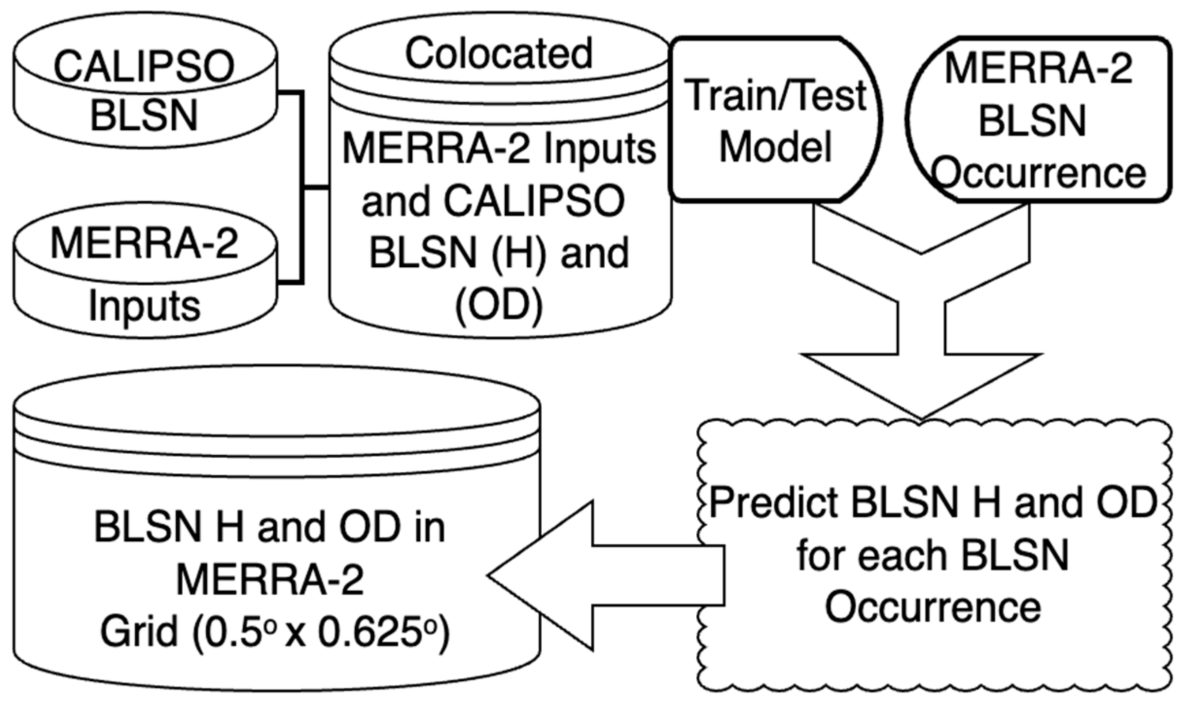
To align CALIPSO blowing snow data with the MERRA-2 grid, a new CALIPSO grid is created by grouping every 50 consecutive data points. Within each grid cell, the height and optical depth values are averaged. The associated dates, latitudes, and longitudes are then matched to the nearest MERRA-2 grid points, allowing identification of co-located training and testing data. The data integration from MERRA-2, CALIPSO BLSN along with the complete process involved in estimating H and OD is illustrated in Figure 2.

2.2. Model Selection

In the context of this study, it was essential to select a representative period that posed both a challenge and an opportunity for model optimization. October was chosen as the focus month for training and evaluating the ML models due to its transitional nature in Antarctica’s seasonal cycle. This month experiences a wide range of atmospheric conditions, including frequent and variable blowing snow events occurring during both day and night. Such variability introduces complexity, making October an ideal month to assess the robustness and generalization capability of the predictive models. Consequently, the October data from 2007 to 2016 were utilized for training and validation in this study.
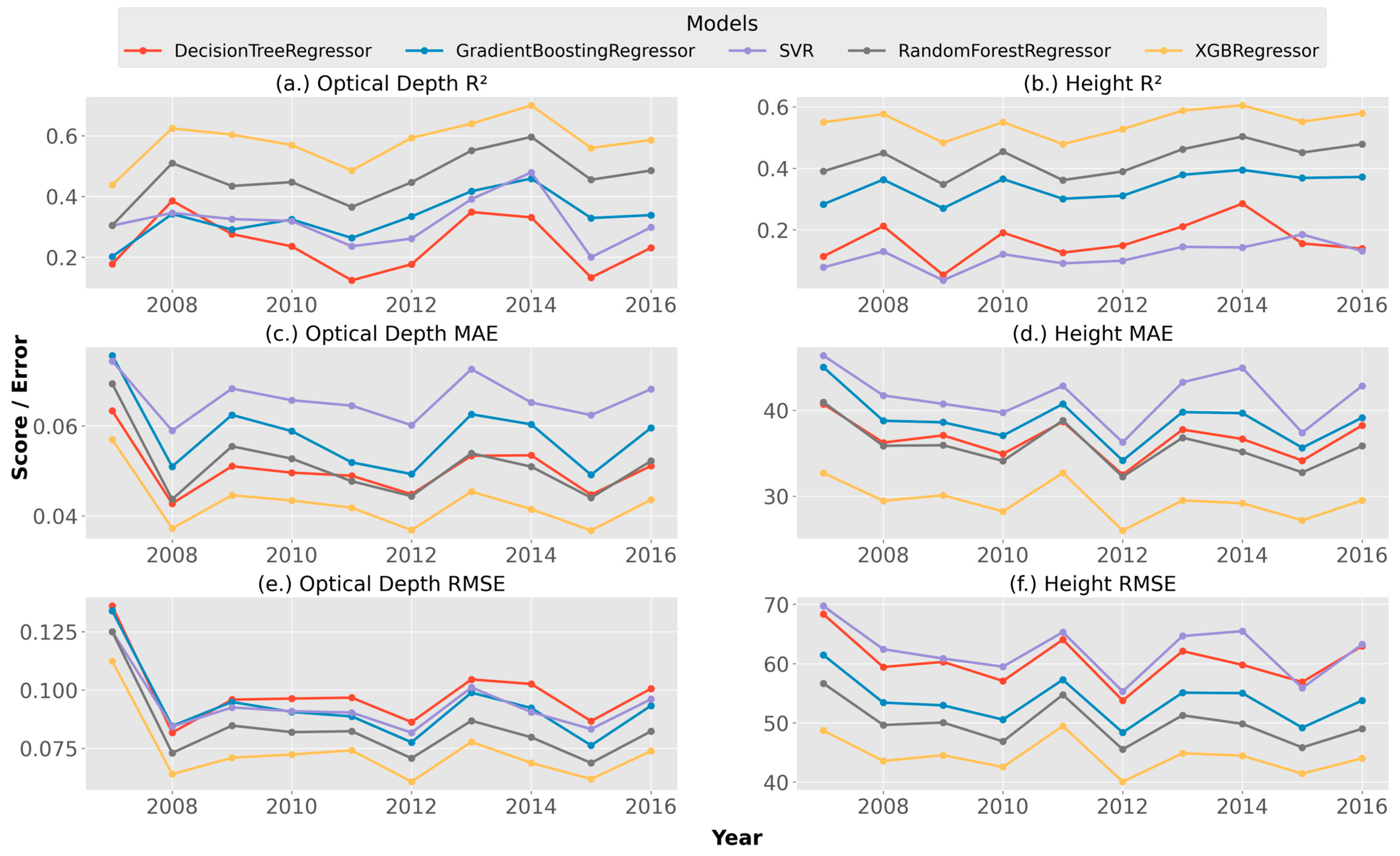
An 80% training and 20% testing data split was adopted for each month to identify the most suitable models. Potential variables outlined in Table 1 were utilized to select the model that optimally captures the predictive efficiency of the input variables concerning the target variables, BLSN H, and OD. Five widely used regression models (Figure 3) were chosen for a comprehensive evaluation of the 20% testing data, assessing their performance metrics, including R2 score, root mean square error (RMSE), and mean absolute error (MAE). The computed metrics for both H and OD are presented in Figure 3. Among the various regression models, Random Forest (RF) and Extreme Gradient Boosting (XGBoost) demonstrated better performance, exhibiting higher R2 scores along with lower RMSE and MAE, as illustrated in Figure 3a–f. Notably, XGBoost showed slightly better performance across all three categories, leading to its selection for the comprehensive training process.

2.3. XGBoost Model

XGBoost is a gradient-boosted decision tree algorithm introduced by Chen and Guestrin in 2016 [38], designed for efficient and scalable ML. It utilizes boosting, which combines multiple weak learners to create a strong learner, effectively reducing training errors and enhancing model performance. The algorithm sequentially builds trees, where each new tree is trained to correct the errors of the previous ones, thereby focusing on misclassified instances. The model is expressed through additive functions, where predictions are based on a combination of tree outputs. The objective function combines a loss function with a regularization term to prevent overfitting. The XGBoost leverages parallelization to improve computational speed, making it suitable for handling large datasets efficiently. The model’s output is the weighted sum of predictions from all trees, allowing it to learn from past errors and produce robust predictions. The regularization term in the objective function accounts for tree complexity, balancing model fit and complexity to prevent overfitting.

2.4. Input Feature Selection

To identify the most impactful features contributing to BLSN H and OD, a comprehensive analysis is conducted. Initially, a set of surface parameters, including pressure, temperature, wind components, and geopotential height, along with the bottommost layer variables, is established as the primary input set (Inputs1). The temperature gradient is calculated using temperatures at the 2 m and the lowest model levels. Subsequently, additional layers are incorporated, introducing parameters such as pressure level, wind components, specific humidity, etc., from higher atmospheric levels (above surface levels). These successive additions, illustrated in Table 2 results in the creation of input sets ‘Inputs2’ through ‘Inputs4’. This progressive approach yields a total of four sets of input variables, each building upon the preceding layer, with the goal of identifying the most influential combination of features associated with BLSN events. In Table 2, the numbers in the acronym list of variables represent the corresponding level numbers.
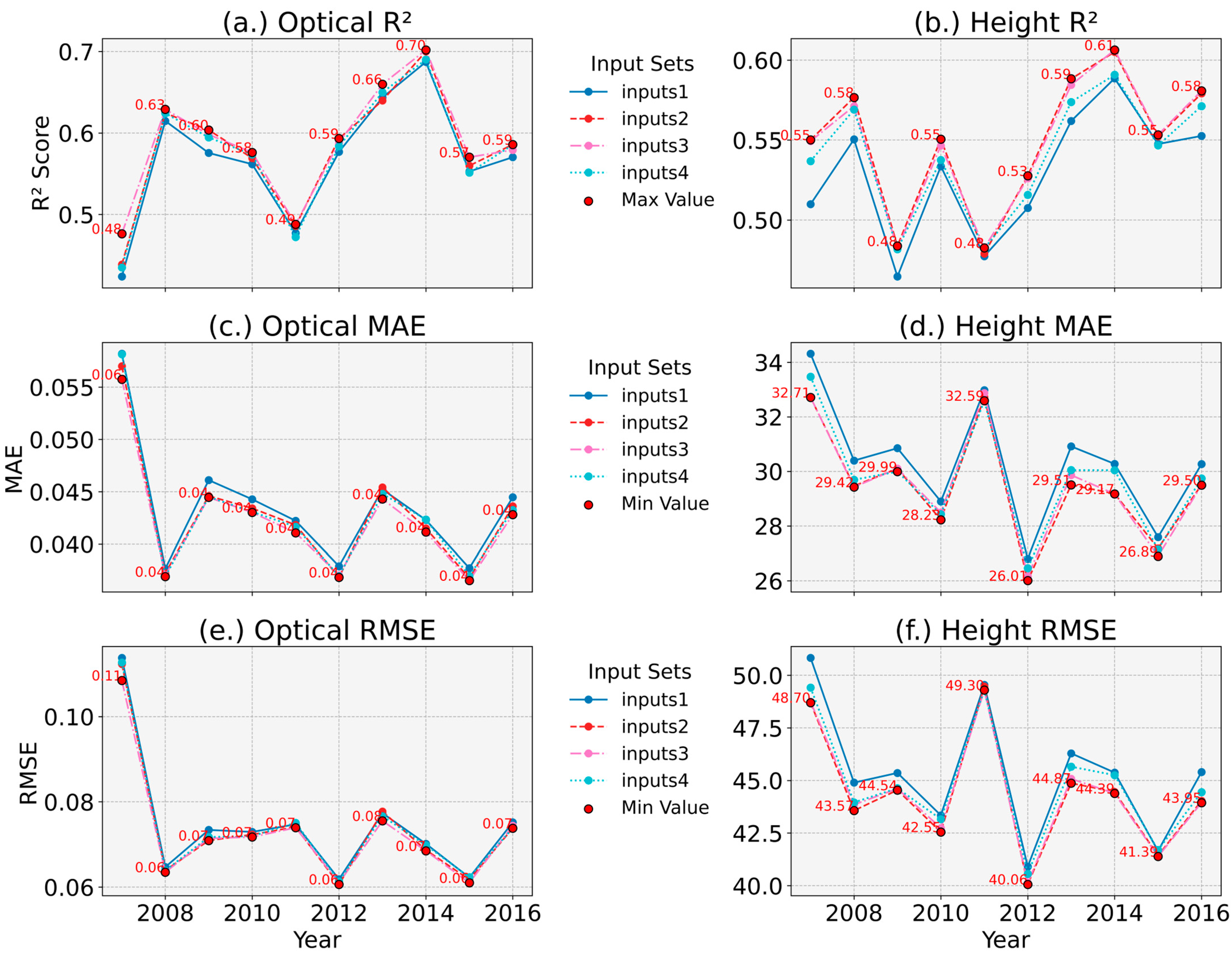
The model was tested using four different input sets (Inputs 1 to Inputs 4), with data from October months spanning 2007 to 2016. The dataset was split into 80% for training and 20% for testing. The objective was to identify the optimal input set for predicting BLSN H and OD. Upon analysis, ‘Inputs 2’ consistently exhibited slightly higher R2 scores and lower RMSE and MAE for both H and OD predictions. This led us to adopt the combinations specified in ‘Inputs2’. Figure 4 illustrates the performance metrics for OD and H predictions: panels (a) and (b) represent the R2 score, (c) and (d) show MAE, and (e) and (f) RMSE, respectively.

3. Results

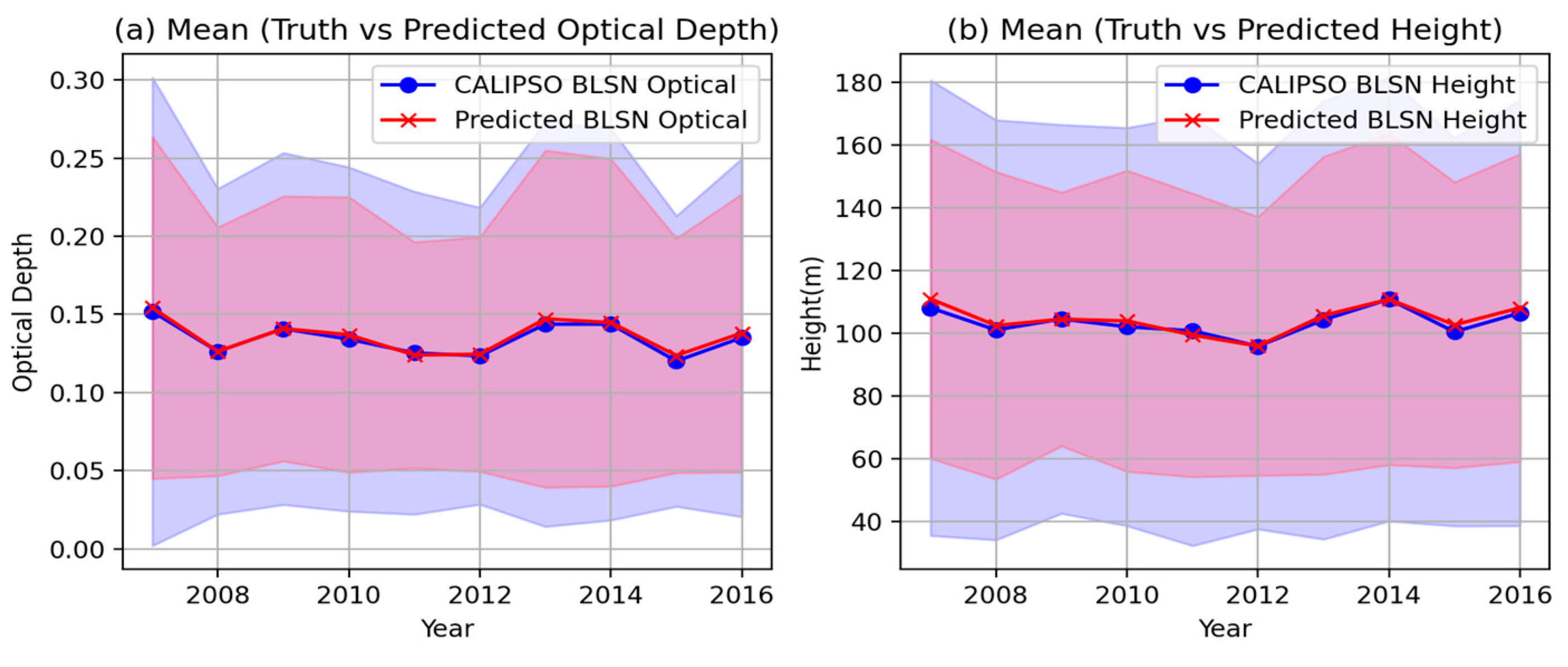
The R2 scores for H and OD for October 2010 are approximately 0.55 and 0.58 (Figure 4a,b), respectively. We tested the model for each October from 2007 to 2016 to analyze variations in H and OD during those years. The predicted H and OD values for the test data of each month, and their averages, along with the standard error, are illustrated in Figure 5a,b. The results indicate that the true values have higher variability than the predicted values. The model performs well in the mid-range or high-density values but is less effective at the lower and higher ends of the H and OD spectrum. Nonetheless, there is strong agreement between the predicted and actual averages of the test data, as shown in Figure 5a,b.
Shapley values, a concept in game theory, were introduced by Shapley in 1953 as a method for fairly allocating benefits among participants in cooperative games [39]. SHAP (SHapley Additive exPlanations) value is a useful method that works on cooperative game theory and is recently gaining attention due to the transparency and interpretability of ML models [40]. It illustrates how the presence or absence of each feature influences the model’s learning process. So, we adopted SHAP based feature importance determination method. In Figure 6, the SHAP-based feature importance analysis for the H and OD-trained model during October 2010 is presented. As expected, Figure 6a,b show that surface pressure and V10M wind are among the most important factors influencing the determination of BLSN H and OD. Surface pressure variations are closely linked to wind patterns, as high or low surface pressure affects wind directions and speeds, hence impacting snow particle transport. The strength and direction of the wind are crucial in snow transport and redistribution, influencing H and OD. These atmospheric factors, among others, shape blowing snow dynamics, and the model appears adept at capturing the relationships between these features, highlighting wind dynamics as essential in shaping blowing snow optical properties. These rankings may vary for other months.
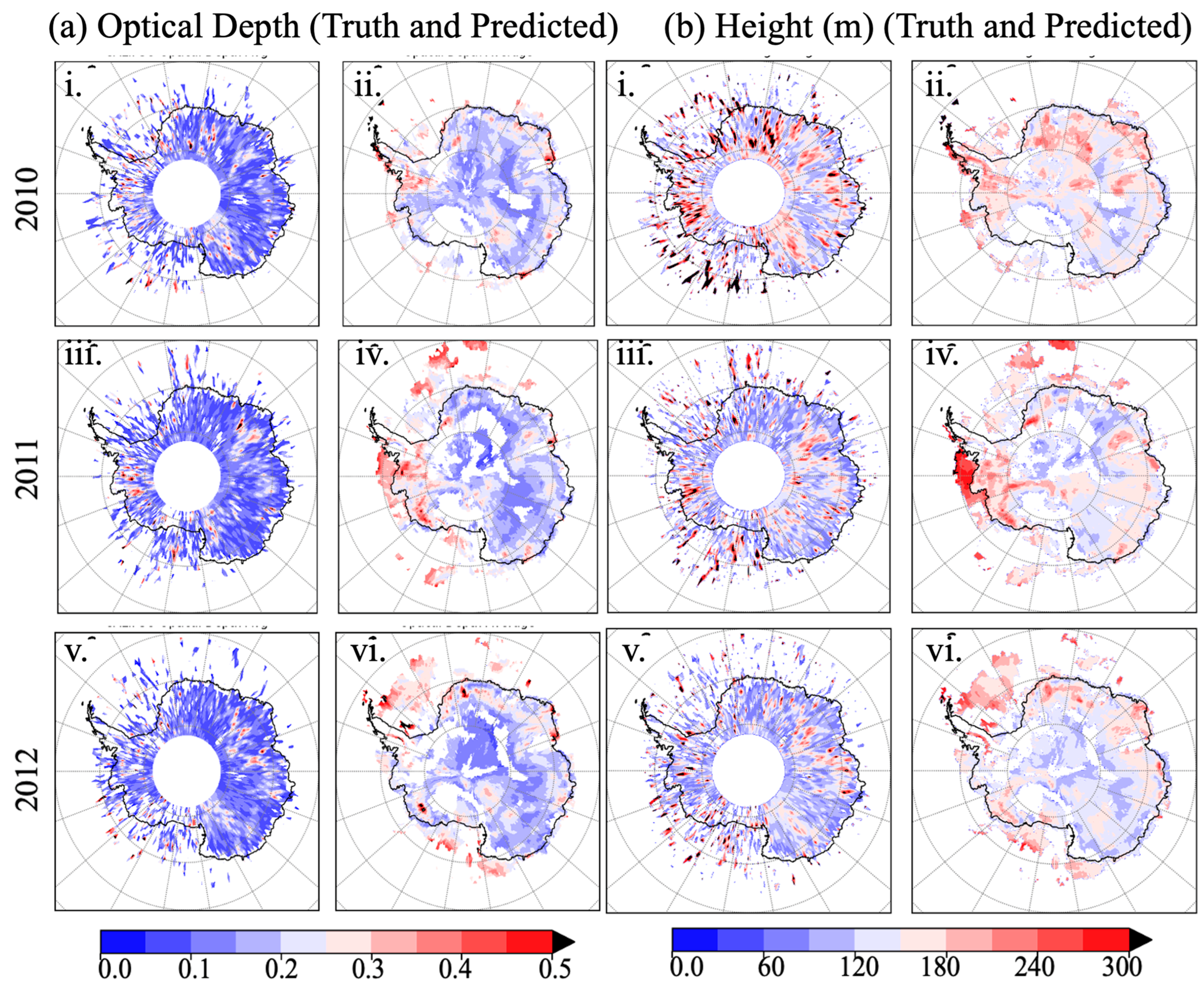
For this study, a separate ML model is developed for each month over the years where CALIPSO ground truth values are available, following the conventional 80–20% split for training and testing. The trained models are applied to the MERRA-2 data. In Figure 7 presents two panels, (a) and (b), illustrating the monthly average BLSN OD and H for October, based on CALIPSO observations and model predictions over a sampled 3-year period (2010, 2011, and 2012). In both panels, subpanels (i), (iii), and (v) show CALIPSO-derived values, while (ii), (iv), and (vi) display the corresponding predicted monthly averages for OD and H. It shows agreement with CALIPSO grid-averaged H and OD and accurately identifies hot spots with higher BLSN H and OD. This analysis focuses exclusively on land ice and sea ice areas. The average H and OD distribution reveals that the BLSN layer attains greater heights in coastal and sea ice regions compared to the interior of Antarctica. The distribution of blowing snow is shaped by the influence of katabatic winds [27,28,31,41,42], linking to the BLSN layers. Katabatic winds are downslope winds that are driven by gravity toward the coast from the high interior of the continent. These winds pick up momentum and speed as they descend from higher altitudes, frequently reaching greater speeds close to the coast [43]. The production of a thicker and higher blowing snow layer along the coastal regions is facilitated by the increased wind speed, which also influences the distribution of snow particles. The presence of sea ice in the analysis further contributes to the observed patterns.
The slight differences in Figure 7 between the true and predicted values can be attributed to several factors. The H and OD values are estimated for the BLSN diagnosed by Bhatta and Yang (2025) [34], which includes BLSN under cloudy conditions, where blowing snow frequency can be different than those under clear conditions. Additionally, MERRA-2 produces BLSN uniformly for each grid at hourly intervals, whereas CALIPSO samples the Earth with ground tracks with a single pixel width. Therefore, differences between the truth and model predictions are expected.
As presented in Figure 4, the model scores for BLSN H and OD across all of Octobers from 2007 to 2016. The R2 score for H peaks at ~0.61, with a minimum of ~0.48. Similarly, for OD, the R2 score reaches ~0.70 with a minimum of ~0.49. Given the model’s promising performance on split test data, we explored its application to the extended MERRA-2 years, where CALIPSO ground truth values are unavailable. Instead of the traditional 80–20% split, we assessed the model’s adaptability in months without ground truth, focusing on long-term predictions for the MERRA-2 era (1980–present), H, and OD. To evaluate this, we trained the model for one month and tested it in the same month in different years (e.g., training in October 2010 and testing in Octobers of other years). The performance dropped significantly, with some months showing R2 scores below 0.10 s. This suggests a need for more diverse input features and additional training data to capture patterns in new datasets. To improve predictive performance, we combined data from October months between 2007 and 2016 (excluding October 2014) for training. This comprehensive dataset aimed to test the model’s performance specifically on the untouched October 2014 dataset. This approach evaluates the model’s predictive capability beyond initial training months and assesses its effectiveness in years lacking CALIPSO truth data. The resulting R2 scores improved, although they did not reach the levels observed in the 80–20 split tests of the same months as shown. We further enhanced the model by identifying interacting terms and incorporating new features, such as wind shear for both U and V (U70-U10M and V70-V10M). Adjusting some hyperparameters led to R2 scores of ~0.30 for H and ~0.31 for OD in 2014. Similarly, tested on 2008 October test data, it yielded the R2 score of ~0.34 for H and ~0.23 for OD, as shown in Table 3.
So, for a long-term estimation of BLSN data for the entire MERRA-2, aggregating all data from 2007 to 2016 for each month is better than a single-month trained model. This method involves training on decadal data for each month, resulting in 12 separate models. This approach enables the estimation of BLSN H and OD over Antarctic land ice and sea ice from 1980 to the present in the MERRA-2 grid. The framework is technically applicable to years prior to 2007 (since MERRA-2 inputs exist), but predictive performance may vary, and historical outputs should be interpreted with caution, especially in the absence of ground-truth data.

4. Summary

Blowing Snow (BLSN) is a crucial component in the polar region, significantly influencing surface mass balance (SMB). This study addresses the data gap in BLSN height and optical depths over Antarctica, expanding CALIPSO coverage to the MERRA-2 grid from 1980 to the present.
To fill this void, we demonstrate that Machine Learning (ML) can serve as an effective approach by training models using CALIPSO truth values and identifying influential atmospheric parameters from MERRA-2. The model selection involved testing various regressor models, with the XGBoost standing out as the most effective. Subsequently, we tested different input combinations, finding that a combination of the MERRA-2 surface layer and the second layer above surface parameters performed better. This led to the identification of 21 influential parameters, including wind components, temperature gradients, and surface pressure, in predicting BLSN height and optical depth (OD). The monthly trained model can estimate hourly MERRA-2-based BLSN height and optical depth, as evidenced by various metrics tests conducted from October 2007 to 2016, yielding R2 scores of approximately 0.49 to 0.61 for height and 0.48 to 0.70 for OD. This capability enables the expansion of BLSN data coverage to the pole for each hour within a grid of 0.5° by 0.625°.
It further demonstrates the potential for long-term MERRA-2 data generation by training monthly models on 2007–2016 data, resulting in 12 height and 12 optical depth regressors applicable from 1980 onward.
Surface pressure and wind are the high-ranked features in SHAP value feature evaluation in predicting BLSN height and optical depth. Surface pressure variations strongly influence wind patterns, impacting the transport of snow particles. These atmospheric factors play a central role in shaping blowing snow events, and the model captures these relationships. The coastal region and sea ice region attain a higher BLSN layer than the interior region of Antarctica. Models trained with this refined approach are applied across the entire MERRA-2 era, enabling the generation of hourly Blowing Snow (BLSN) height and optical depth datasets.

Author Contributions

S.B. drafted the paper, designed the machine learning, and result analysis. Y.Y. concept design and paper edits. All authors have read and agreed to the published version of the manuscript.

Funding

This study is supported by NASA’s Modeling, Analysis, and Prediction (MAP) and CloudSat/CALIPSO Science programs, both managed by David Considine.

Institutional Review Board Statement

Not applicable.

Informed Consent Statement

Not applicable.

Data Availability Statement

The datasets used in this study are publicly available. Modeled estimated data will also be published in an open data source. The CALIPSO Lidar Level 2 Antarctic blowing snow product, version 1.00, is directly accessible at (https://opendap.larc.nasa.gov/opendap/CALIPSO/LID_L2_BlowingSnow_Antarctica-Standard-V1-00/contents.html) last accessed on 12 April 2025. MERRA-2 data are available online (https://disc.gsfc.nasa.gov/datasets?project=MERRA-2) last accessed on 12 April 2025, managed by the NASA Goddard Earth Sciences (GES) Data and Information Services Center (DISC).

Acknowledgments

The authors thank the three anonymous reviewers for their valuable and constructive reviews.

Conflicts of Interest

The authors declare no conflicts of interest.

References

  1. Palm, S.P.; Yang, Y.; Spinhirne, J.D.; Marshak, A. Satellite Remote Sensing of Blowing Snow Properties over Antarctica. J. Geophys. Res. Atmos. 2011, 116. [Google Scholar] [CrossRef]
  2. Loeb, N.A.; Kennedy, A. Blowing Snow at McMurdo Station, Antarctica During the AWARE Field Campaign: Surface and Ceilometer Observations. J. Geophys. Res. Atmos. 2021, 126, e2020JD033935. [Google Scholar] [CrossRef]
  3. Xiao, J.; Bintanja, R.; Déry, S.J.; Mann, G.W.; Taylor, P.A. An Intercomparison Among Four Models Of Blowing Snow. Bound.-Layer Meteorol. 2000, 97, 109–135. [Google Scholar] [CrossRef]
  4. Mellor, M. Blowing Snow; CRREL Monograph, Part III, Section A3c; U.S. Army Corps of Engineers, Cold Regions Research and Engineering Laboratory: Hanover, NH, USA, 1965; 79p. [Google Scholar]
  5. Sigmund, A.; Melo, D.B.; Dujardin, J.; Nishimura, K.; Lehning, M. Parameterizing Snow Sublimation in Conditions of Drifting and Blowing Snow. J. Adv. Model. Earth Syst. 2025, 17, e2024MS004332. [Google Scholar] [CrossRef]
  6. Palm, S.P.; Kayetha, V.; Yang, Y.; Pauly, R. Blowing Snow Sublimation and Transport over Antarctica from 11 Years of CALIPSO Observations. Cryosphere 2017, 11, 2555–2569. [Google Scholar] [CrossRef]
  7. Das, I.; Bell, R.E.; Scambos, T.A.; Wolovick, M.; Creyts, T.T.; Studinger, M.; Frearson, N.; Nicolas, J.P.; Lenaerts, J.T.M.; van den Broeke, M.R. Influence of Persistent Wind Scour on the Surface Mass Balance of Antarctica. Nat. Geosci 2013, 6, 367–371. [Google Scholar] [CrossRef]
  8. Gadde, S.; van de Berg, W.J. Contribution of Blowing-Snow Sublimation to the Surface Mass Balance of Antarctica. Cryosphere 2024, 18, 4933–4953. [Google Scholar] [CrossRef]
  9. Bintanja, R. Snowdrift Sublimation in a Katabatic Wind Region of the Antarctic Ice Sheet. J. Appl. Meteorol. 2001, 40, 1952–1966. [Google Scholar] [CrossRef]
  10. Lenaerts, J.T.M.; van den Broeke, M.R.; Déry, S.J.; van Meijgaard, E.; van de Berg, W.J.; Palm, S.P.; Sanz Rodrigo, J. Modeling Drifting Snow in Antarctica with a Regional Climate Model: 1. Methods and Model Evaluation. J. Geophys. Res. Atmos. 2012, 117. [Google Scholar] [CrossRef]
  11. Déry, S.J.; Tremblay, L.-B. Modeling the Effects of Wind Redistribution on the Snow Mass Budget of Polar Sea Ice. J. Phys. Oceanogr. 2004, 34, 258–271. [Google Scholar] [CrossRef]
  12. Gossart, A.; Palm, S.P.; Souverijns, N.; Lenaerts, J.T.M.; Gorodetskaya, I.V.; Lhermitte, S.; van Lipzig, N.P.M. Importance of Blowing Snow During Cloudy Conditions in East Antarctica: Comparison of Ground-Based and Space-Borne Retrievals Over Ice-Shelf and Mountain Regions. Front. Earth Sci. 2020, 8. [Google Scholar] [CrossRef]
  13. Palm, S.P.; Kayetha, V.; Yang, Y. Toward a Satellite-Derived Climatology of Blowing Snow Over Antarctica. J. Geophys. Res. Atmos. 2018, 123, 10301–10313. [Google Scholar] [CrossRef]
  14. Lesins, G.; Bourdages, L.; Duck, T.J.; Drummond, J.R.; Eloranta, E.W.; Walden, V.P. Large Surface Radiative Forcing from Topographic Blowing Snow Residuals Measured in the High Arctic at Eureka. Atmos. Chem. Phys. 2009, 9, 1847–1862. [Google Scholar] [CrossRef]
  15. Mann, G.W.; Anderson, P.S.; Mobbs, S.D. Profile Measurements of Blowing Snow at Halley, Antarctica. J. Geophys. Res. Atmos. 2000, 105, 24491–24508. [Google Scholar] [CrossRef]
  16. Li, L.; Pomeroy, J.W. Probability of Occurrence of Blowing Snow. J. Geophys. Res. Atmos. 1997, 102, 21955–21964. [Google Scholar] [CrossRef]
  17. Huang, J.; Jaeglé, L. Wintertime Enhancements of Sea Salt Aerosol in Polar Regions Consistent with a Sea Ice Source from Blowing Snow. Atmos. Chem. Phys. 2017, 17, 3699–3712. [Google Scholar] [CrossRef]
  18. Zwally, H.J.; Schutz, B.; Abdalati, W.; Abshire, J.; Bentley, C.; Brenner, A.; Bufton, J.; Dezio, J.; Hancock, D.; Harding, D.; et al. ICESat’s Laser Measurements of Polar Ice, Atmosphere, Ocean, and Land. J. Geodyn. 2002, 34, 405–445. [Google Scholar] [CrossRef]
  19. Walden, V.P.; Warren, S.G.; Tuttle, E. Atmospheric Ice Crystals over the Antarctic Plateau in Winter. J. Appl. Meteorol. Climatol. 2003, 42, 1391–1405. [Google Scholar] [CrossRef]
  20. Taylor, P. The Thermodynamic Effects of Sublimating, Blowing Snow in the Atmospheric Boundary Layer. Bound.-Layer Meteorol. 1998, 89, 251–283. [Google Scholar] [CrossRef]
  21. Schmidt, R.A. Sublimation of Wind-Transported Snow: A Model; Rocky Mountain Forest and Range Experiment Station, Forest Service: Fort Collins, CO, USA; U.S. Department of Agriculture: Washington, DC, USA, 1972.
  22. Déry, S.J.; Yau, M.K. Large-Scale Mass Balance Effects of Blowing Snow and Surface Sublimation. J. Geophys. Res. Atmos. 2002, 107, ACL 8-1–ACL 8-17. [Google Scholar] [CrossRef]
  23. Frezzotti, M.; Scarchilli, C.; Becagli, S.; Proposito, M.; Urbini, S. A Synthesis of the Antarctic Surface Mass Balance during the Last 800 Yr. Cryosphere 2013, 7, 303–319. [Google Scholar] [CrossRef]
  24. Déry, S.J.; Yau, M.K. A Bulk Blowing Snow Model. Bound.-Layer Meteorol. 1999, 93, 237–251. [Google Scholar] [CrossRef]
  25. Gallée, H.; Guyomarc’h, G.; Brun, E. Impact Of Snow Drift On The Antarctic Ice Sheet Surface Mass Balance: Possible Sensitivity To Snow-Surface Properties. Bound.-Layer Meteorol. 2001, 99, 1–19. [Google Scholar] [CrossRef]
  26. Essery, R.; Li, L.; Pomeroy, J. A Distributed Model of Blowing Snow over Complex Terrain. Hydrol. Process. 1999, 13, 2423–2438. [Google Scholar] [CrossRef]
  27. Scarchilli, C.; Frezzotti, M.; Grigioni, P.; De Silvestri, L.; Agnoletto, L.; Dolci, S. Extraordinary Blowing Snow Transport Events in East Antarctica. Clim. Dyn. 2010, 34, 1195–1206. [Google Scholar] [CrossRef]
  28. Pomeroy, J.; Jones, H. Wind-Blown Snow: Sublimation, Transport and Changes to Polar Snow. In Chemical Exchange Between the Atmosphere and Polar Snow; Springer: Berlin/Heidelberg, Germany, 1996; pp. 453–489. [Google Scholar]
  29. Mott, R.; Vionnet, V.; Grünewald, T. The Seasonal Snow Cover Dynamics: Review on Wind-Driven Coupling Processes. Front. Earth Sci. 2018, 6. [Google Scholar] [CrossRef]
  30. Palm, S.P.; Yang, Y.; Herzfeld, U.; Hancock, D.; Hayes, A.; Selmer, P.; Hart, W.; Hlavka, D. ICESat-2 Atmospheric Channel Description, Data Processing and First Results. Earth Space Sci. 2021, 8, e2020EA001470. [Google Scholar] [CrossRef]
  31. Yang, Y.; Kiv, D.; Bhatta, S.; Ganeshan, M.; Lu, X.; Palm, S. Diagnosis of Antarctic Blowing Snow Properties Using MERRA-2 Reanalysis with a Machine Learning Model. J. Appl. Meteorol. Climatol. 2023, 62, 1055–1068. [Google Scholar] [CrossRef]
  32. Chung, Y.-C.; Bélair, S.; Mailhot, J. Blowing Snow on Arctic Sea Ice: Results from an Improved Sea Ice–Snow–Blowing Snow Coupled System. J. Hydrometeorol. 2011, 12, 678–689. [Google Scholar] [CrossRef]
  33. Leonard, K.C.; Maksym, T. The Importance of Wind-Blown Snow Redistribution to Snow Accumulation on Bellingshausen Sea Ice. Ann. Glaciol. 2011, 52, 271–278. [Google Scholar] [CrossRef]
  34. Bhatta, S.; Yang, Y. Selection and Optimization of a Machine Learning Algorithm for Antarctic Blowing Snow Diagnosis Using MERRA-2 Reanalysis. Artif. Intell. Earth Syst. 2025, 4. [Google Scholar] [CrossRef]
  35. Bosilovich, M.G.; Lucchesi, R.; Suarez, M. MERRA-2: File Specification 2015. Available online: https://ntrs.nasa.gov/citations/20150019760 (accessed on 25 February 2025).
  36. Gelaro, R.; McCarty, W.; Suárez, M.J.; Todling, R.; Molod, A.; Takacs, L.; Randles, C.A.; Darmenov, A.; Bosilovich, M.G.; Reichle, R.; et al. The Modern-Era Retrospective Analysis for Research and Applications, Version 2 (MERRA-2). J. Clim. 2017, 30, 5419–5454. [Google Scholar] [CrossRef]
  37. Mahesh, A.; Eager, R.; Campbell, J.R.; Spinhirne, J.D. Observations of Blowing Snow at the South Pole. J. Geophys. Res. Atmos. 2003, 108, 785–794. [Google Scholar] [CrossRef]
  38. Chen, T.; Guestrin, C. Xgboost: A Scalable Tree Boosting System; Association for Computing Machinery: New York, NY, USA, 2016; pp. 785–794. [Google Scholar]
  39. Shapley, L.S. A Value for N-Person Games; Princeton University Press: Princeton, NJ, USA, 1953. [Google Scholar]
  40. Lundberg, S.M.; Erion, G.G.; Lee, S.-I. Consistent Individualized Feature Attribution for Tree Ensembles. arXiv 2018, arXiv:1802.03888. [Google Scholar]
  41. Barral, H.; Genthon, C.; Trouvilliez, A.; Brun, C.; Amory, C. Blowing Snow in Coastal Adélie Land, Antarctica: Three Atmospheric-Moisture Issues. Cryosphere 2014, 8, 1905–1919. [Google Scholar] [CrossRef]
  42. Kodama, Y.; Wendler, G.; Gosink, J. The Effect of Blowing Snow on Katabatic Winds in Antarctica. Ann. Glaciol. 1985, 6, 59–62. [Google Scholar] [CrossRef]
  43. Parish, T.R. A Numerical Study of Strong Katabatic Winds over Antarctica. Mon. Weather Rev. 1984, 112, 545–554. [Google Scholar] [CrossRef]
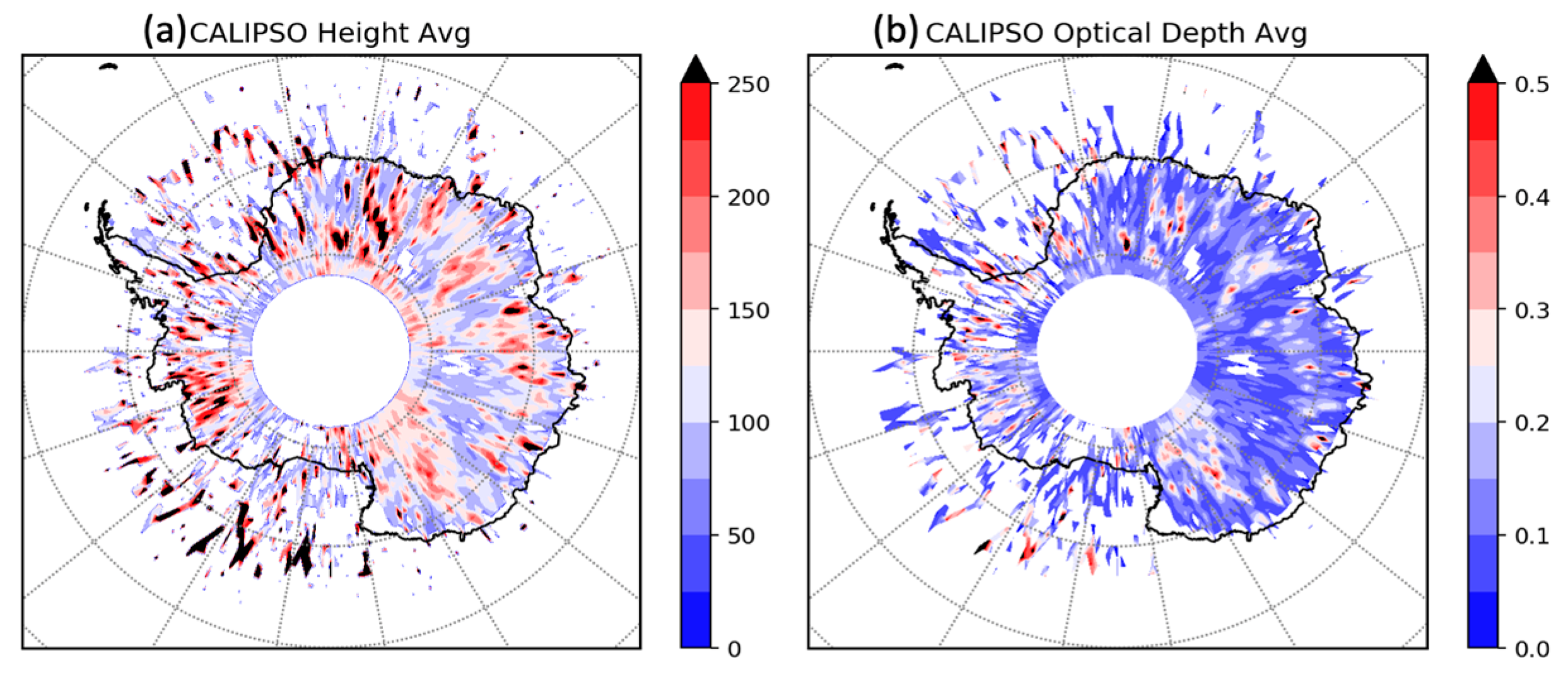
Figure 1. CALIPSO average blowing snow (a) height and (b) optical depth for October 2010.
Atmosphere 16 00760 g001
Figure 2. Flowchart illustrating the process of data merging and integration of input variables with corresponding truth values to identify optimal feature combinations for developing a predictive model of blowing snow height (H) and optical depth (OD) within the MERRA-2 grid framework.
Atmosphere 16 00760 g002
Figure 3. Model comparison for predicting blowing snow height (H) and optical depth (OD) using input features listed in Table 1. Panels (a,c,e) show OD prediction results, while panels (b,d,f) correspond to H prediction. Each panel presents model performance based on R2 score, mean absolute error (MAE), and root mean square error (RMSE).
Atmosphere 16 00760 g003
Figure 4. Predictive performance of the XGBoost regression model across four input variable combinations. Panel (a) shows the R2 score for optical depth (OD), and (b) for height (H). Panels (c) and (d) show mean absolute error (MAE), and panels (e) and (f) show root mean square error (RMSE), for OD and H, respectively.
Atmosphere 16 00760 g004
Figure 5. Models were trained and evaluated separately for each month: (a) BLSN Optical Depth and (b) BLSN Height show the monthly mean observed (truth) and predicted values, along with their standard errors: light red for predicted and light blue for truth from October 2007 to 2016.
Atmosphere 16 00760 g005
Figure 6. SHAP-based feature importance of trained model for October 2010 (a) Optical Depth and (b) Height.
Atmosphere 16 00760 g006
Figure 7. Monthly averaged CALIPSO-observed and model-predicted blowing snow (BLSN) optical depth (OD) and height (H) for October of 2010, 2011, and 2012. Panel (a) shows BLSN OD, with subplots (i,iii,v) representing CALIPSO observations and subplots (ii,iv,vi) showing the corresponding model predictions. Panel (b) presents BLSN height, following the same structure: observed values in subplots (i,iii,v) and predicted values in subplots (ii,iv,vi).
Atmosphere 16 00760 g007
Table 1. Preliminary MERRA-2 input variables used in optimal feature combination.
Bottom 4 LayersSurface
Pressure (PL)Pressure (PS)
Temperature (T)Temperature (T2M)
Specific Humidity (Qv)Eastward wind (U10M)
Eastward Wind (U)Northward wind (V10M)
Northward Wind (V)Specific Humidity (Qv2M)
Total Latent Energy Flux (EFLUX)Temperature Gradient (2M) (Tg)
Sensible Heat Flux From Turbulence (HFLUX)Geo. Potential Height
Table 2. Progressive sets of input variables starting from base surface features, with additional atmospheric layers added incrementally to form four distinct input sets.
Variable GroupInputs1Inputs2Inputs3Inputs4
PSPSPSPSPS
HFLUXHFLUXHFLUXHFLUXHFLUX
EFLUXEFLUXEFLUXEFLUXEFLUX
PHISPHISPHISPHISPHIS
Temp GradientTemp_GRTemp_GRTemp_GRTemp_GR
U10MU10MU10MU10MU10M
V10MV10MV10MV10MV10M
QV2MQV2MQV2MQV2MQV2M
T2MT2MT2MT2MT2M
U LevelsU71U71, U70U71, U70, U69U71, U70, U69, U68
V LevelsV71V71, V70V71, V70, V69V71, V70, V69, V68
T LevelsT71T71, T70T71, T70, T69T71, T70, T69, T68
QV LevelsQV71QV71, QV70QV71, QV70, QV69QV71, QV70, QV69, QV68
PL LevelsPL71PL71, PL70PL71, PL70, PL69PL71, PL70, PL69, PL68
OMEGA LevelsOMEGA71OMEGA71, OMEGA70OMEGA71, OMEGA70, OMEGA69OMEGA71, OMEGA70, OMEGA69, OMEGA68
Table 3. Model R2 scores using October data (2007–2016) with Leave-One-Year-Out Validation (2008 and 2014 hold out).
Model Trained on October
2007–2016, Holdout:
Height
R2 Score
Optical Depth R2 Score
2008 October0.340.23
2014 October0.300.31
Disclaimer/Publisher’s Note: The statements, opinions and data contained in all publications are solely those of the individual author(s) and contributor(s) and not of MDPI and/or the editor(s). MDPI and/or the editor(s) disclaim responsibility for any injury to people or property resulting from any ideas, methods, instructions or products referred to in the content.