Construction of a High-Resolution Temperature Dataset at 40–110 KM over China Utilizing TIMED/SABER and FY-4A Satellite Data

Abstract

This study aims to develop a high-resolution temperature dataset from 40 km to 110 km over China by machine learning techniques, with a horizontal resolution of 0.5° × 0.5° and vertical resolution of 1 km, utilizing measurements from SABER onboard the Thermosphere, Ionosphere, Mesosphere Energetics, and Dynamics (TIMED) and Fengyun 4A (FY-4A) satellites. Accurate temperature profiles play a critical role in understanding the atmospheric dynamics and climate change. However, because of the limitation of traditional detecting methods, the measurements of the upper stratosphere and mesosphere are rare. In this study, a new method is developed to construct a high-resolution temperature dataset over China in the middle atmosphere based on the XGBoost technique. The model’s performance is also validated based on rocket observations and ERA5 reanalysis data. The results indicate that the model effectively captures the characteristics of the vertical and seasonal variations in temperature, which provide a valuable opportunity for further research and improvement of climate models. The model demonstrates the highest accuracy below 80 km with RMSE < 12 K, while its performance decreases above 100 km, where RMSE can exceed 20 K, indicating optimal performance in the upper stratosphere and lower mesosphere regions.

1. Introduction

Atmospheric temperature is a crucial parameter to describe the thermal structure, dynamic perturbations, and climatological features of the whole atmosphere. It essentially determines the distributions of the geopotential and wind field, which further drive the global circulation, and affects the vertical propagation of energy and momentum. Accurate temperature data is essential for understanding the atmospheric dynamic processes, as well as coupling between different atmospheric layers [1]. However, due to the limitation of detecting methods, the temperature observations in the middle and upper atmosphere are rare, especially in the upper stratosphere and mesosphere (~40–100 km). Thus, establishing a reliable long-term temperature dataset with a large spatial coverage is the most fundamental topic in atmosphere dynamics.

Understanding the coupling between different atmospheric layers is fundamental for accurate temperature modeling in the MLT region. The troposphere and lower stratosphere significantly influence the middle and upper atmospheric layers through multiple mechanisms: (1) upward propagation of gravity waves generated by tropospheric convection and topographic forcing; (2) planetary wave interactions that transport energy and momentum vertically; (3) tidal oscillations originating from solar heating in the troposphere; (4) meridional circulation patterns that connect surface climate variability to mesospheric dynamics. These coupling processes justify the inclusion of lower atmospheric data (ERA5) in our modeling approach, as surface and stratospheric conditions provide essential boundary conditions for MLT temperature variations.

Ground-based observations from radars and lidars, which are significantly affected by local environmental and weather conditions, show limited spatial coverage. To obtain the global temperature profiles in the mesosphere and lower thermosphere (MLT) region, satellite observations are the most important data source. The Sounding of the Atmosphere using Broadband Emission Radiometry (SABER) on the Thermosphere, Ionosphere, Mesosphere Energetics, and Dynamics (TIMED) satellite has been providing temperature data of 16–120 km since 2002 [2]. The Michelson Interferometer for Global High-Resolution Thermospheric Imaging (MIGHTI) onboard the Ionospheric Connection Explorer (ICON) satellite has two identical sensor units, MIGHTI-A and MIGHTI-B, which can be used to retrieve temperatures at 90–115 km [3,4,5]. Reanalysis datasets are significant for studying the physical processes and dynamic changes in the atmospheric temperature, such as those provided by ERA5 and MERRA2, which are capable of describing the distribution and variations in temperature in the middle atmosphere up to ~80 km (0.1 hpa).

ERA5 reanalysis data is a valuable tool for validating temperature datasets, particularly in specialized applications like astronomical site characterization. For instance, Shikhovtsev et al. utilized ERA5 temperature profiles, along with wind and humidity data, to train neural networks for estimating astronomical seeing at the Maidanak site [6]. Their study involved rigorous validation by comparing ERA5 temperatures and wind speed profiles against radiosonde data from the nearby Dzhambul station, revealing mean absolute temperature errors of 1.3 °C in winter and 1.7 °C in summer within the lower atmosphere. They also identified specific limitations, such as ERA5’s difficulty in accurately reproducing thin surface-based temperature inversions and mesojets. Complementing this, Shikhovtsev et al. employed ERA5 data, including temperature-derived parameters like humidity for precipitable water vapor (PWV), to statistically characterize atmospheric conditions relevant to telescope performance at another site [7]. These studies underscore ERA5’s value as a globally consistent, high-resolution benchmark. While it exhibits quantifiable errors in complex terrain and specific atmospheric regimes, validation against ground truth, such as radiosonde data, provides critical insights into its accuracy and limitations.

However, their main limitations regarding altitude range are sparse data, discontinuities and relatively large biases in the upper atmosphere above 50 hPa, as well as insufficient vertical resolution to capture small-scale structures of the upper atmosphere.

At present, long-lasting measurements of temperature in the MTL region with relatively high spatial and temporal resolutions are still rare. The primary objective of this study is to construct a high-resolution temperature dataset in the MLT region over China from 2019 to 2023 based on observations of SABER/TIMED and Fengyun 4A (FY-4A) satellites, as well as ERA5 reanalysis data. Herein, we focused on the geographical region of China and its surroundings, which is defined by a latitudinal range of 15° N to 55° N, a longitudinal range of 70° E to 140° E, and an altitudinal range of 40 km to 110 km. The horizontal resolution is 0.5° × 0.5° and the vertical resolution is 1 km. To analyze the collected data and validate the model’s performance, machine learning techniques, specifically XGBoost, are utilized. By addressing the existing gaps in temperature data, this study aims to provide a valuable data resource for further atmospheric research and to improve the accuracy of the model of the middle and upper atmospheres.

2. Data and Method

2.1. Data Description

TIMED spacecraft was launched in December 2001 with an orbital inclination of ~74° at 625 km. It flies around the Earth in about 1.6 h. The ascending (descending) local time at the same latitudes are similar for a specific day. Complete local time coverage is achieved in about 60 days due to the spacecraft ‘s processional motion of ∼12 min every day. SABER onboard the TIMED satellite is a broadband radiometer that has been providing global temperature profiles from the stratosphere to the lower thermosphere since early 2002. It views the atmosphere 90° to the satellite velocity vector of the TIMED spacecraft and measures Earth limb emission profiles in 10 selected spectral bands ranging from 1.27 to 15 μm. Thus, the coverage of SABER data is either 83° N to 52° S or 83° S to 52° N, depending on the yaw cycles. The yaw modes of the spacecraft alternate once every two months. A more detailed description of SABER is provided by Russell et al. [8].

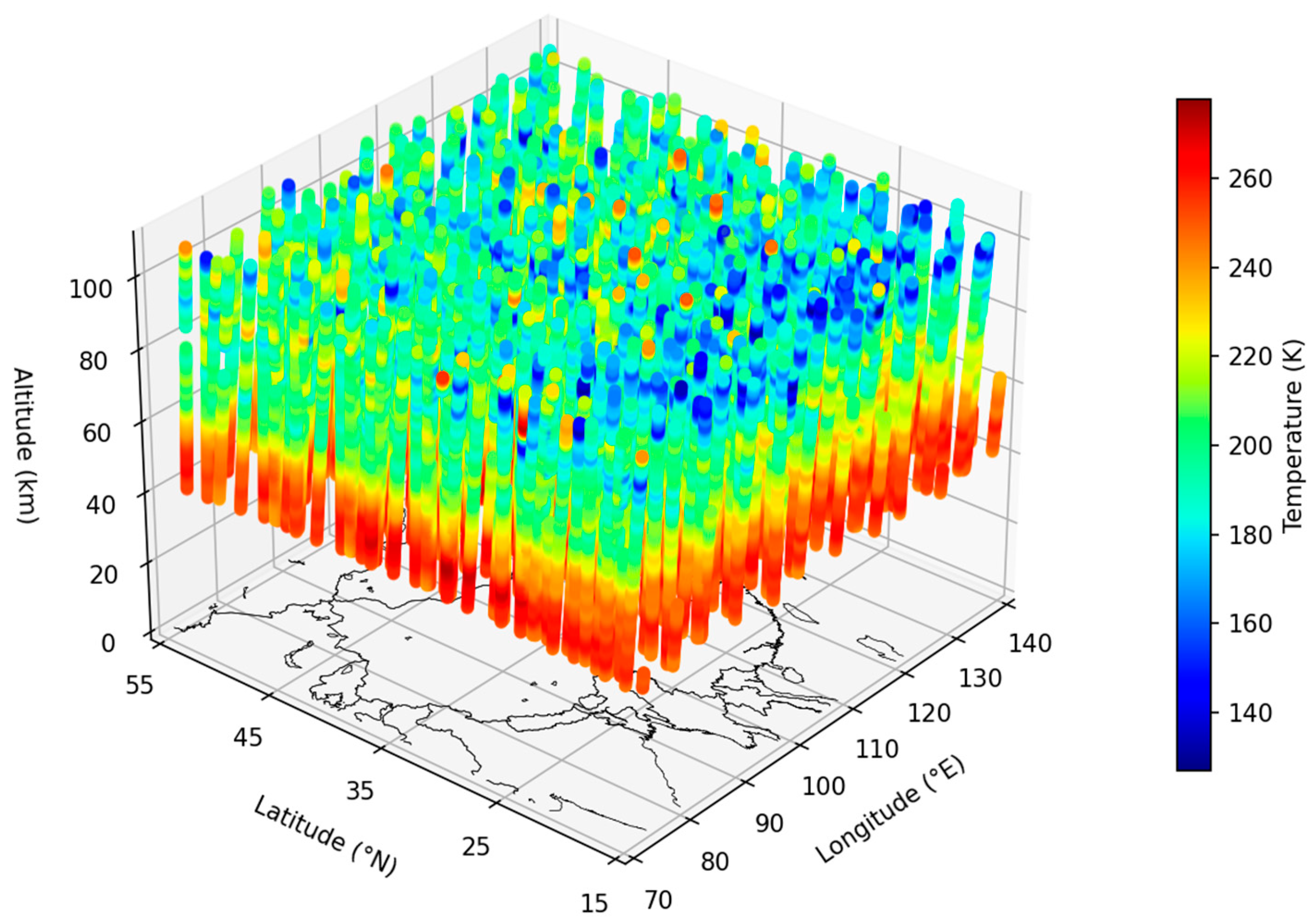
The SABER instrument has been providing vertical profiles of temperature since 2002 [9,10,11,12], which plays a pivotal role in advancing our understanding of the MLT region. The retrieved temperature profiles of SABER have a vertical resolution somewhat better than 2 km, but they are oversampled on a vertical grid of ∼380 m [13]. It provides a unique opportunity for us to establish an estimation model to generate a high-resolution and long-term global temperature dataset. Herein, we use the SABER temperature data at 40–110 km from 2019 to 2023. Figure 1 displays the data collected by SABER in January 2019. The spatial coverage demonstrates the potential to construct a comprehensive dataset for the middle and upper atmosphere.

Fengyun-4A (FY-4A) satellite is China’s second-generation geostationary meteorological satellite, launched in 2016 to provide improved imagery, sounding, lightning mapping, and space environment monitoring [14]. Its key instruments include the Advanced Geosynchronous Radiation Imager (AGRI) for high-resolution visible and infrared imaging, the Geostationary Interferometric Infrared Sounder (GIIRS) for atmospheric temperature and humidity profiling, and the Lightning Mapping Imager (LMI) for detecting lightning flashes. In this study, the altitude, land type, and land–sea mask data from FY-4A are utilized to train our model, which has a spatial resolution of 4 km. The FY-4A-derived parameters (altitude, land type, and land–sea mask) serve as auxiliary features in the XGBoost model, providing geographical and topographical context that enhances temperature estimation accuracy. These parameters are used as training inputs for the model through a spatial collocation method, which identifies points geographically proximal to SABER observations in latitude–longitude space. More details about the input features are listed in

Table 1. All the input variables of our model.

Variable	Source	Resolution	Physical Significance
Temperature	SABER/TIMED	~2 km vertical	Target variable
Latitude	SABER/TIMED	-	Geographic position
Longitude	SABER/TIMED	-	Geographic position
Altitude	FY-4A	4 km	Surface elevation
Land type	FY-4A	4 km	Surface characteristics
Land–sea mask	FY-4A	4 km	Surface type identifier

.

2.2. Data Fusion Method

We use XGBoost to build our estimation model. XGBoost is a novel algorithm introduced in 2016 by Chen and Guestrin [15]. Similar to the Random Forest (RF) algorithm, XGBoot is an ensemble method based on many weak learners. The ensemble technique of XGBoost is Boosting, which differs from the Bagging utilized by RF. Learners of RF are parallel and share the same data distribution. However, learners of XGB are serial, and focus more on samples that are predicted incorrectly. The XGBoost model is very efficient in computation, with its training time being 1/7 of that of RF model under the same hyperparameter settings. The hyperparameters of XGBoost comprise the number of trees and max depth of the trees.

Feature importance is obtained from the impurity reduction. For a given node m with left and right child nodes, the impurity reduction ${Gain}_m$ is expressed as

$${Gain}_m=i_m-(w_{left}·i_{left}+w_{right}·i_{right})$$

(1)

where i_m, i_left, and i_right are the impurity of node m, as well as its left and right child nodes, respectively. w is the weight, defined as the share of the parent’s examples in a child node (e.g., w_left = N_left/N_m, where N is the number of examples in a node or leaf). In order to derive the total impurity reduction in a given feature f in tree t, we need to sum across all the nodes $m\in M_f^{\left(t\right)}$, which performs a split on that feature f and divide it by the total impurity reduction number of all nodes of that tree. Eventually, the total importance of feature f is calculated across all trees t in the random forest with a total number of trees T, and expressed as

$${Importance}_f={\displaystyle \frac{1}{T}}{\sum }_{t=1}^T{Importance}_f^{\left(t\right)}$$

(2)

where ${Importance}_f^{\left(t\right)}$ is the importance of a given feature f in tree t, and expressed as

$${Importance}_f^{\left(t\right)}={\displaystyle \frac{{\sum }_{m\in M_f^{\left(t\right)}}{Gain}_m}{{\sum }_f{\sum }_{m\in M_f^{\left(t\right)}}{Gain}_m}}$$

(3)

To validate our model estimations, we employ several statistical metrics, including Root Mean Square Error (RMSE), correlation coefficient (R), Mean Relative Error (MRE), and Mean Absolute Error (MAE).

To prevent overfitting and ensure the generalizability of the XGBoost model, several strategies were implemented. First, the dataset was divided into a training set and a testing set with a ratio of 80:20. A relatively large proportion of the data was allocated to the testing set to evaluate the model’s performance on unseen data more rigorously. Second, extensive hyperparameter tuning was conducted to optimize model performance and avoid both overfitting and underfitting. The tuning process involved searching for suitable hyperparameter combinations by comparing model performance metrics—such as error rates—on both the training and testing datasets. A model suffering from overfitting typically exhibits significantly lower errors on the training set than on the testing set. By analyzing the distribution of errors under various hyperparameter settings, we were able to identify an optimal configuration that maintains consistent performance across both datasets, thus mitigating the risk of overfitting.

To quantitatively evaluate the performance of the model, several statistical metrics were employed, including the coefficient of determination (R²), Root Mean Square Error (RMSE), Mean Absolute Error (MAE), and Mean Relative Error (MRE).

R² measures the proportion of the variance in the observed data that is predictable from the model output. A value closer to 1 indicates a stronger agreement between predicted and observed values.

$$R^2=1-{\displaystyle \frac{\sum {(y_i-{\widehat{y}}_i)}^2}{\sum {(y_i-{\overline{y}}_i)}^2}}$$

(4)

where yᵢ is the observed value, ŷᵢ is the predicted value, and ȳ is the mean of observed values.

RMSE represents the square root of the average squared differences between predictions and observations. It is sensitive to large errors and thus emphasizes the impact of significant deviations.

$$\mathrm{R}\mathrm{M}\mathrm{S}\mathrm{E}=\sqrt{{\sum }_{i=1}^n{\displaystyle \frac{{{(\widehat{y}}_i-y_i)}^2}{n}}}$$

(5)

MAE calculates the average of the absolute differences between predictions and observations, providing an intuitive measure of overall prediction accuracy that is less sensitive to outliers than RMSE.

$$\mathrm{M}\mathrm{A}\mathrm{E}={\displaystyle \frac{1}{n}}{\sum }_{i=1}^n\left|{\widehat{y}}_i-y_i\right|$$

(6)

MRE expresses the average absolute error as a percentage of the observed values, offering a normalized measure of model performance across different value ranges.

$$\mathrm{M}\mathrm{R}\mathrm{E}={\displaystyle \frac{1}{n}}{\sum }_{i=1}^n{\displaystyle \frac{\left|{\widehat{y}}_i-y_i\right|}{y_i}}\times 100\%$$

(7)

3. Temporal Spatial Coverage

Before constructing the model, we conducted a visual analysis of the representativeness of the dataset. Figure 2, Figure 3 and Figure 4 illustrate the distribution of sample frequencies across different seasons in the planes of longitude and latitude, latitude and altitude, and longitude and altitude, respectively. The region under investigation encompasses a spatial domain defined by the latitudinal range of 15° N to 55° N, the longitudinal range of 70° E to 140° E, and the altitudinal range of 40 km to 110 km. This three-dimensional domain was discretized into a grid system composed of cubic cells. The horizontal dimensions of each grid cell were set to 0.5° in both latitude and longitude, while the vertical dimension was fixed at 1 km in altitude. This gridding approach enables the systematic partitioning of the region of interest into a series of discrete volumetric elements for further investigation and analysis. It is evident from Figure 2, Figure 3 and Figure 4 that there are no significant data gaps for all the four seasons. The highest sampling frequency occurs during summer, while the lowest sampling frequency is observed in autumn.

4. Results

4.1. Model Performance

In this study, we utilized a dataset comprising a total of 6,608,473 samples to evaluate the performance of our model. The dataset was divided into training and testing subsets with an 80%/20% ratio. This division was used to ensure that the model is trained on a substantial portion of the data while retaining an adequate amount for unbiased performance evaluation.

To assess the estimation accuracy of the model, we employed several evaluation metrics, including Root Mean Square Error (RMSE), R-squared (R²), Mean Absolute Error (MAE), and Mean Relative Error (MRE). The results are shown in Figure 5, demonstrating that our model achieves an RMSE of ~11.43, an R² of ~0.86, an MAE of ~7.72, and an MRE of ~3.86%. It indicates that no signs of underfitting or overfitting are exhibited in the model.

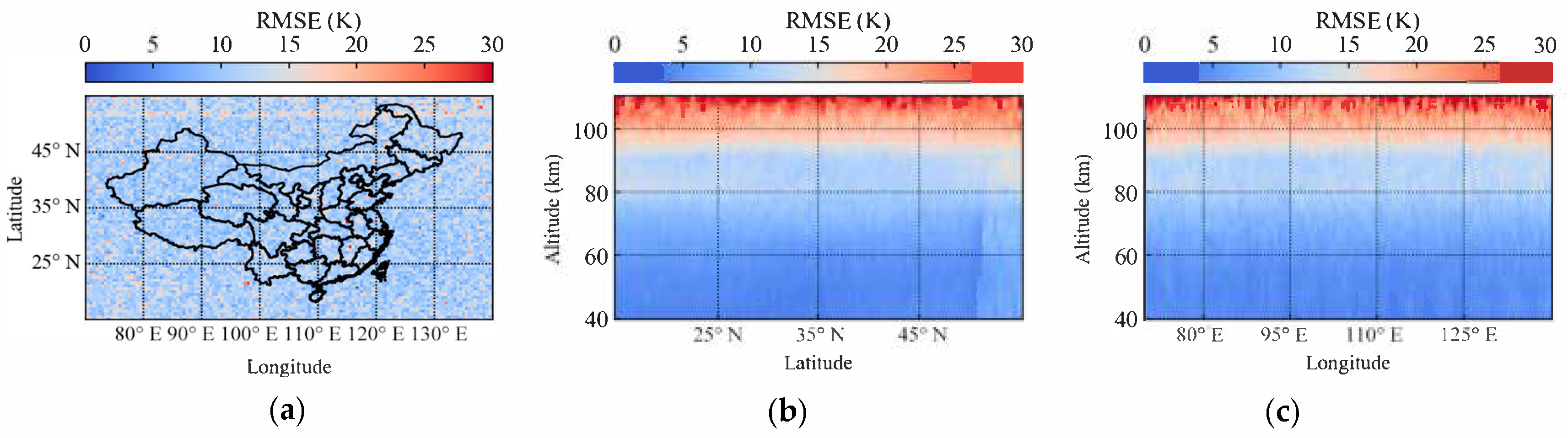
We calculated the spatial distribution of error over China using the RMSE metric, employing the same grid as in Section 3. As shown in Figure 6, there is no evident trend with respect to latitude and longitude, with RMSE primarily remaining below 15. However, the situation differs at different altitudes: below 100 km, RMSE values are significantly lower than 15, while larger errors are observed above 100 km, where RMSE exceeds 20 and can even reach 30.

4.2. Validation on Season

To further validate the performance of our model, we conducted a comparative analysis of the model’s estimations against actual observations across various seasons and time intervals. This analysis allows us to assess the model’s estimation accuracy and its ability to capture seasonal variations, as shown in Figure 7.

We first examined the model’s predictions during the four seasons: spring, summer, autumn, and winter. The results indicated that the model performed at a consistently high level across all four seasons. In each season, the R² value exceeded 0.8, and the RMSE remained below 12, demonstrating the model’s robustness. However, some differences were observed among the seasons. Spring and autumn exhibited relatively lower RMSE values, while spring and summer had higher R² scores. Overall, winter had the weakest performance, while spring yielded the best results. This seasonal variation aligns with the temperature patterns, as spring and summer months typically experience higher temperatures compared to autumn and winter.

4.3. Validation at Low Latitude

Temperature data detected by the first meteorological rocket of the Meridian Space Weather Monitoring Project at Hainan (20° N, 109° E) are used to assess the model’s performance at low latitude in China.

Figure 8 shows that the rocket-decocted profile (green dots) in Hainan aligns well with the model estimates (blue dots), particularly in the altitude range of 40 km to 45 km, where the error remains below 1 K. However, the error increases between 45 km and 50 km, which is characterized by an overestimation with a maximum deviation of approximately 8 K. At altitudes above 40 km, three sample points contained in the ERA5 datasets at 40 km, 44 km, and 48 km, respectively [16]. The estimated results (blue dots) are consistent with the ERA5 temperature (red asterisks) at both 40 km and 44 km. However, a problem of underestimation of ERA5 data is found at 48 km.

4.4. Validation at Middle Latitude

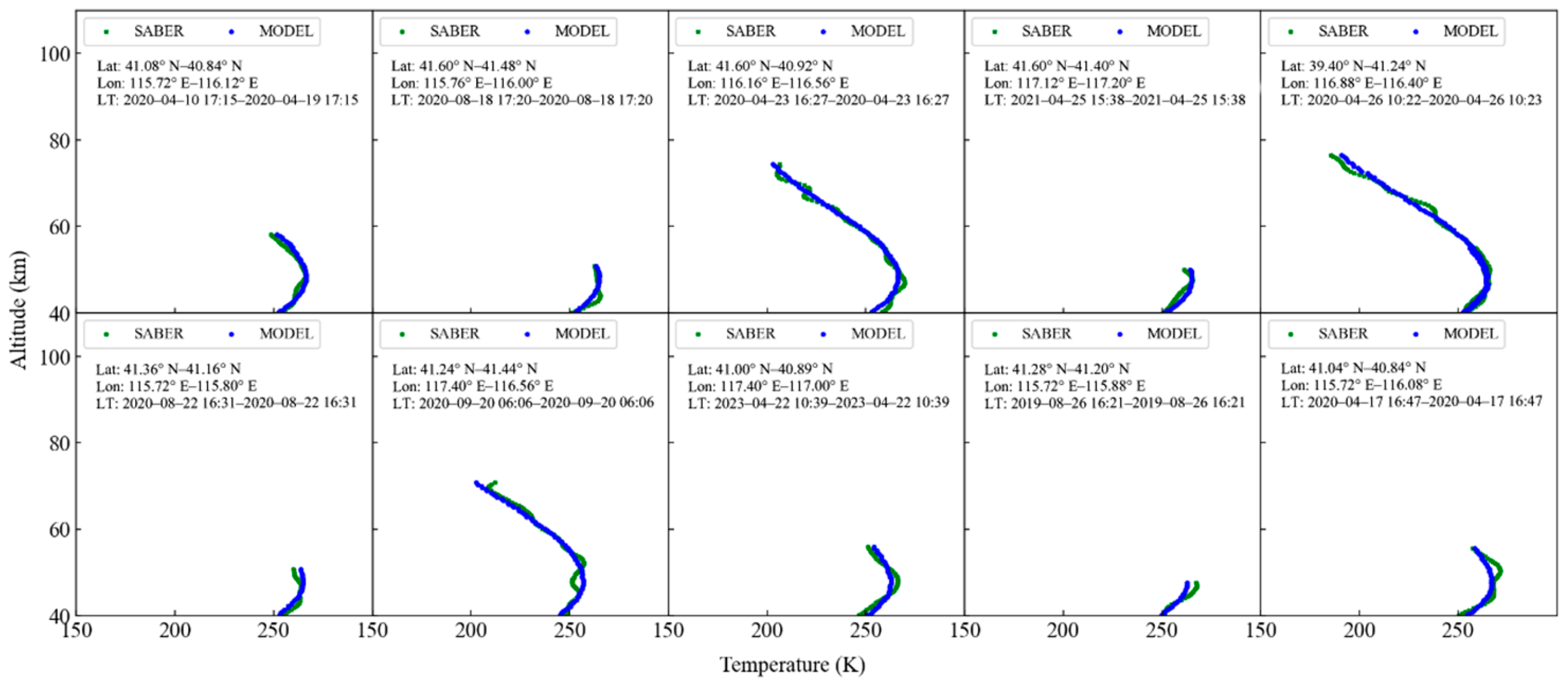
Temperature profiles over Beijing, which is defined by latitudes ranging from 39.4° N to 41.6° N and longitudes from 115.7° E to 117.4° E, obtained by SABER are used to assess the model’s performance at middle latitude in China. According to these geographical conditions, 116 profiles of SABER were identified. Then, we excluded the profiles with a sample number less than 20, and 104 profiles are ultimately selected, comprising a total of 9146 samples collected over five years. We also calculated the error for each profile and identified the ten worst and ten best profiles based on RMSE metrics, as illustrated in Figure 9 and Figure 10, respectively. Figure 9 indicates that our model performs well between 40 and 80 km, with detailed information presented in

Table 2. The best and worst 10 profiles estimation on Beijing.

	WORST10					BEST10
NO.	R	RMSE (K)	MAE (K)	MRE	N	R	RMSE (K)	MAE (K)	MRE	N
1	0.97	40.15	36.04	0.19	22	0.94	2.20	1.83	0.01	48
2	−0.75	35.90	32.42	0.17	41	0.83	2.30	1.84	0.01	29
3	0.93	29.02	27.24	0.15	20	0.99	2.56	2.05	0.01	90
4	0.73	21.62	16.36	0.09	63	0.95	2.57	2.15	0.01	27
5	−0.17	21.06	17.54	0.09	93	1.00	2.61	1.96	0.01	136
6	0.83	20.05	17.53	0.09	44	0.71	2.68	2.33	0.01	28
7	0.80	19.67	16.34	0.09	65	0.99	2.72	2.12	0.01	81
8	0.52	19.52	17.61	0.09	27	0.98	2.83	2.61	0.01	42
9	0.63	19.39	14.06	0.08	55	0.98	3.05	2.47	0.01	20
10	0.59	19.29	15.94	0.09	73	0.95	3.06	2.62	0.01	41

.

Figure 10 shows that our model struggles to capture the variations in the temperature above 80 km, particularly at altitudes exceeding 110 km. This limitation can be attributed to several factors. At a higher layer of the MLT region, especially above 80 km, atmospheric waves play a more important role than at lower altitudes, which may not be well described in our model. Additionally, the sparse availability of data at these elevated altitudes further complicates accurate modeling.

Table 2 presents the detailed metrics for the ten worst and ten best profiles. It is found that the maximum RMSE exceeds 40, while the best profiles have an RMSE of less than 3.

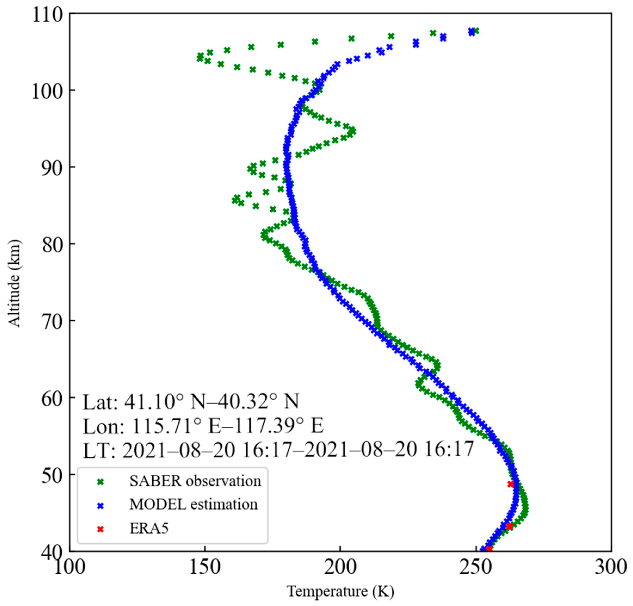
Figure 11 compares the specific profiles of temperature at 16:17 LT 20 August 2021, which are detected by SABER (green crosses), estimated by our model (blue crosses), and obtained from ERA5 dataset (red crosses), respectively. We can see that these three profiles are basically consistent with each other at below 50 km. It can be found that the vertical variation in temperature observed by SABER is generally consistent with that estimated by our model, with only the model estimation showing less small-scale structures. This suggests that the model established in our study is incapable of estimating the small-scale structures of the temperature, especially at above 80 km.

5. Summary and Discussion

Recent research on middle and upper atmosphere temperature retrieval in the 40–110 km altitude range have primarily focused on advancing satellite-based measurement techniques and understanding long-term climate trends in the MLT region. The SABER instrument has been instrumental in providing temperature data from 20 to 110 km altitudes, enabling comprehensive analysis of temperature trends, solar cycle responses, and atmospheric oscillations from 2002 to 2020 [17]. Complementing satellite observations, ground-based lidar systems have emerged as crucial validation tools, with sodium lidar networks being particularly effective for temperature and wind measurements in the MLT region [18].

The objectives of all these research focus on three key areas: developing more accurate retrieval algorithms, validating multi-platform observations, and quantifying climate change impacts in the upper atmosphere. NASA’s ICON/MIGHTI mission has advanced temperature retrieval methodologies using molecular oxygen atmospheric band emissions near 763 nm, providing measurements from 90 to 127 km altitudes during day-time and 90 to 108 km at night [19]. Additionally, machine learning approaches incorporating historical observations and ground-based measurements have been developed to improve atmospheric temperature profile retrieval accuracy [20].

The significance of temperature retrieval in the 40–110 km region extends beyond basic atmospheric science to critical climate change detection. Recent findings reveal dramatic cooling of the MLT region from 2002 to 2019, with temperature decreases of 1.75 to 19 K depending on the altitude [21]. These measurements are essential for understanding upper atmospheric responses to increasing greenhouse gas concentrations, validating climate models, and assessing impacts on satellite operations and space weather predictions. The MLT region serves as a critical indicator of anthropogenic climate change, as it exhibits cooling trends opposite to lower atmospheric warming, providing unique fingerprints of human influence on Earth’s atmospheric system.

In this study, we constructed a high-resolution temperature dataset for the MLT region over China, utilizing data from SABER/TIMED, FY-4A satellite, and ERA5 reanalysis. By employing advanced machine learning techniques, we have established a model that is able to generate reliable temperature profiles across altitudes of 40 to 110 km. The model demonstrated strong performance metrics, including an RMSE of approximately 11.43 K and an R² value around 0.86, indicating its effectiveness in capturing the temperature variations across different seasons and altitudes. Key findings are listed as follows:

• The validation of both training and testing datasets confirms that our model is free from issues of underfitting or overfitting. The close performance metrics observed for both datasets indicate the model’s strong generalization capabilities. This robustness highlights the model’s effectiveness in accurately predicting temperature profiles across various altitudes and seasons, reinforcing its reliability for atmospheric research.
• Seasonal analysis revealed statistically significant differences in model performance. The best results are found in spring (RMSE = 10.92 K, R² = 0.89), while the lowest accuracy (RMSE = 11.89, R² = 0.80) is found in winter. The altitude-dependent performance shows that RMSE is less than 10 K for 85% profiles below 70 km. However, RMSE increases and is larger than 15 K above 90 km for 60% profiles.
• The model’s estimations were validated using observations and reanalysis data, showcasing its robustness in representing the characteristics of the atmospheric temperature. In addition, specific validations at low and middle latitudes over China highlighted the model’s ability to capture local structures of the temperature, with errors generally remaining within acceptable limits.

The establishment of the high-resolution temperature dataset in our study fills a data gap in the MTL region where traditional detecting techniques are limited [22]. Based on this dataset, future studies will need to investigate the long-term trends in the atmospheric temperature and its correlation with global climate patterns.

However, our model still has some limitations: (1) Reduced accuracy above 80 km altitude due to increased atmospheric wave activity and sparse observational data; (2) limited capability in capturing small-scale temperature structures, particularly above the mesopause; (3) dependence on the quality and availability of input datasets, particularly SABER coverage limitations during yaw maneuvers; (4) regional focus limiting global applicability; (5) temporal coverage restricted to 2019–2023, which may not capture long-term climate variability patterns. Further studies will have to take into account more data and improved methods.