Characterization of Historical Aerosol Optical Depth Dynamics Using LSTM and Peak Enhancement Techniques

Abstract

This study addresses the challenges of characterizing aerosol optical depth (AOD) dynamics from satellite observations, which are often hindered by data gaps and variability. A long short-term memory (LSTM) network was trained on an extended AOD dataset from Sicily to capture temporal patterns. The trained model was then applied to AOD data from distinct geographical regions: Cluj-Napoca and the central Mediterranean Sea. While the LSTM effectively captured general seasonal trends, it tended to smooth extreme AOD events. To mitigate this, a post-processing algorithm was developed to enhance the representation of AOD peaks and valleys. This enhancement method refines the characterization of historical AOD, providing a more accurate representation of observed atmospheric variability, particularly in capturing high and low AOD episodes. The results demonstrate the efficacy of the hybrid approach in improving the characterization of AOD dynamics across different regions.

1. Introduction

Atmospheric aerosols play a crucial role in the Earth’s climate system by directly scattering and absorbing solar radiation and indirectly influencing cloud formation and properties [1,2,3]. Precise monitoring and analysis of aerosols’ spatial and temporal variations are essential because of their significant effects on climate, air quality, and public health [4,5]. Satellite remote sensing has become a vital tool for observing aerosol optical depth (AOD) across regional to global scales, providing consistent and long-term datasets that are indispensable for advancing climate and air quality research [6,7,8,9,10]. Cloud cover, acquisition methods, and temporal discontinuities frequently limit satellite-based AOD retrievals [11,12]. Continuous monitoring and forecasting could prove more challenging due to these limitations, particularly in regions where aerosol events are frequent. Advanced machine learning methods, such as LSTM networks tailored for time-series analysis, offer a promising alternative for enhancing AOD prediction accuracy by capturing complex temporal patterns and filling gaps in missing data. The selection of LSTM networks was grounded in their architectural strength in modeling temporal dependencies within sequential data. While traditional approaches such as ARIMA can effectively capture linear components and regular seasonality, they often fail to represent the nonlinear and long-memory dynamics characteristic of AOD fluctuations. Other machine learning techniques—such as random forest or SVR—have shown merit in related tasks, but they lack the intrinsic temporal modeling capacity that LSTMs provide. In contrast, LSTM networks retain information across time steps, making them well-suited for satellite-based AOD series, where lagged dependencies and seasonal transitions are critical. Furthermore, by improving the spatial resolution of AOD predictions, these innovative machine-learning algorithms can enable more thorough aerosol event monitoring. Researchers can improve the overall accuracy and dependability of AOD predictions by fusing machine-learning models with satellite-based observations.

NASA’s MODIS sensors onboard Terra (since 2000) and Aqua (since 2002) have provided a consistent, long-term record of global aerosol observations [13]. With wide swath coverage (2330 km, ±55°), they deliver near-daily data at different times—Terra in the morning (10:30 LT) and Aqua in the afternoon (13:30 LT)—supporting diurnal aerosol studies [13]. MODIS uses 36 spectral bands across various resolutions (250 m–1 km), and retrieves AOD via three main algorithms: dark target (for vegetated areas and the ocean), deep blue (for bright land), and MAIAC [13,14,15]. Unlike DT and DB, MAIAC processes time-series data over fixed grids, allowing it to better handle complex or bright surfaces through multi-angle analysis and surface BRF retrievals [15,16]. This leads to more accurate aerosol estimates, especially in challenging conditions. MAIAC has been validated globally against AERONET, with generally good agreement, though accuracy varies with factors such as aerosol type, loading, and view geometry [11,12,16,17,18,19,20,21,22,23,24,25,26]. It performs well over vegetation, bright land, and during smoke events [15,16,18], making it a valuable tool for regional aerosol studies, air quality assessments, and PM estimation [20,21,27,28,29,30].

Artificial intelligence (AI), machine learning (ML), and especially deep learning (DL) are increasingly enhancing satellite-based AOD retrieval by capturing complex, non-linear patterns beyond the reach of traditional algorithms [31,32]. Transformer-based models, such as TMAT [33] and AeroTrans-Landsat [31], directly retrieve AOD from multi-angle, multi-spectral data without heavy reliance on surface or aerosol assumptions [34]. These models also integrate meteorological inputs and underused spectral bands to boost accuracy [35,36,37]. Beyond retrieval, AI aids in post-processing existing AOD products, enabling efficient correction and reanalysis [36]. Pre-trained DL models further help in data-scarce regions, extracting meaningful patterns where ground validation is limited [37].

Despite these advancements, several challenges exist in employing AI, ML, and DL for satellite AOD retrieval. One major challenge is the sensitivity of these models to fluctuations in both surface and atmospheric conditions [32]. Models trained on data from one region might face difficulties in accurately predicting AOD in new spatiotemporal domains due to substantial variations in natural conditions and the influence of anthropogenic emissions such as dust and haze [32]. The availability of sufficient and accurately labeled training data remains a critical factor [38], as the performance of these data-driven models heavily relies on the quality and representativeness of the data they are trained on [39].

Satellite-derived AOD, frequently sourced from the MODIS instruments at temporal resolutions ranging from daily to monthly intervals [40], represents a cornerstone dataset for understanding atmospheric composition, air quality dynamics, and climate system interactions. However, its effective utilization is often hampered by observational gaps and complex spatiotemporal variability. Addressing these challenges, long short-term memory (LSTM) neural networks have garnered significant attention, owing to their inherent architecture designed to capture long-range temporal dependencies crucial for analyzing time-series satellite observations. Their application permeates multiple facets of AOD research, starting with environmental impact analysis. LSTMs directly contribute to public health assessments by enabling the prediction of surface air pollutants strongly correlated with AOD, such as PM_2.5 and NO₂ [39,40].

While ML use in AOD prediction is expanding, studies applying advanced models such as the LSTM remain relatively few. Still, recent research shows strong potential. A hybrid SARIMA–LSTM model, optimized with PSO, effectively separated linear and nonlinear AOD components in Delhi, outperforming traditional models [41]. Similarly, CNN–LSTM and ConvLSTM architectures have been used to predict dust storm dynamics using environmental data, enhancing spatial and temporal accuracy [42]. In North Bengal, MODIS AOD combined with meteorological inputs proved effective for PM₁₀ estimation via various ML models [43]. LSTM networks applied to MERRA-2 data also captured seasonal AOD patterns more accurately than conventional approaches, showing promise in data-scarce regions [44].

Building on recent findings, the present study examines the use of LSTM networks to address observational gaps and improve the temporal consistency of monthly AOD data. Under the constraint of limited satellite observations, the investigation assesses the capacity of machine learning techniques to support more reliable aerosol monitoring frameworks across three geographically distinct regions. The results indicate that LSTM models effectively capture complex temporal patterns in AOD, providing a robust method for improving aerosol observation. By employing machine learning to mitigate data limitations and refine the temporal resolution of AOD predictions, this work contributes to ongoing advancements in remote sensing and atmospheric monitoring.

2. Methodology

This study employs a machine learning approach, specifically, a long short-term memory (LSTM) network combined with targeted post-processing techniques, to characterize the dynamics of aerosol optical depth (AOD) derived from satellite observations. To evaluate the capacity of a simple, sequence-driven model to generalize across distinct climatological regimes, we trained an LSTM exclusively on Sicily, a region with a well-defined, seasonal AOD signature. We then applied it without retraining to regions with markedly different aerosol profiles: a continental urban setting (Cluj-Napoca) and a marine environment (central Mediterranean Sea). The rationale was to test whether a model trained on clear seasonality can capture transferable dynamics or if domain-specific learning is essential. Importantly, post-processing enhancement was developed to correct the known LSTM bias of smoothing seasonal extrema, providing a hybrid solution to improve the representation of characteristic peaks and valleys in historical data.

2.1. Data Description and Preprocessing

2.1.1. Study Regions

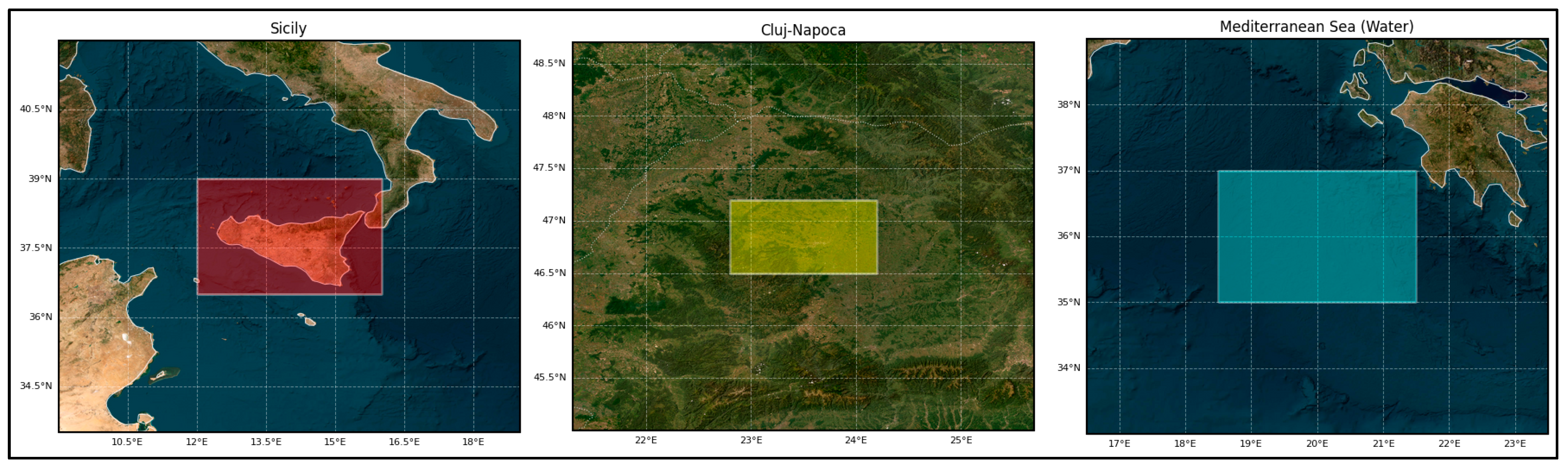
Three distinct geographical areas seen in Figure 1 were central to this investigation. Firstly, Sicily, Italy, delineated by the approximate bounding box [12.0° E, 36.5° N, 16.0° E, 39.0° N], served as the primary region for initial data exploration, comprehensive model development, and subsequent training phases. This region utilized an extended historical dataset, potentially spanning 2000–2018, to ensure the model captured long-term variability and robust seasonal patterns. Secondly, Cluj-Napoca, Romania, defined by the bounding box [22.8° E, 46.5° N, 24.2° E, 47.2° N], was selected as a representative continental European urban area, presenting aerosol characteristics and meteorological conditions contrasting with the Mediterranean environment [45,46,47]. Thirdly, the central Mediterranean Sea within the approximate bounding box [10.0° E, 34.0° N, 20.0° E, 38.0° N] was selected as a maritime analysis region subject to influences from sea salt aerosols, long-range atmospheric transport phenomena, including Saharan dust events [48], and emissions from shipping activities.

2.1.2. Data Acquisition

Monthly Level 3 AOD data were procured from the Moderate Resolution Imaging Spectroradiometer (MODIS) Terra sensor, specifically utilizing the MODIS/006/MOD08_M3 product, which provides global data at a 1 × 1 degree spatial resolution [49]. Data acquisition and initial spatial aggregation were efficiently managed using the Google Earth Engine (GEE) platform [50]. The temporal scope of the data collection extended from January 2000 to December 2023, facilitating the analysis of long-term AOD variability and seasonality. The principal variable extracted was Aerosol_Optical_Depth_Land_Mean_Mean_550 (AOD at 550 nm). Additionally, other potentially relevant variables such as Aerosol_Optical_Depth_Land_Ocean_Mean_Mean, Deep_Blue_Aerosol_Optical_Depth_550_Land_Mean_Mean, Deep_Blue_Angstrom_Exponent_Land_Mean_Mean, Aero-sol_Optical_Depth_Small_Ocean_Mean_Mean_550, and Cloud_Fraction_Mean_Mean were extracted where available. The GEE processing involved filtering the image collection by date for the specified period and subsequently calculating the monthly mean value of each variable within the defined bounding box for each study region using the ee.Image.reduceRegion() function with ee.Reducer.mean(). A spatial scale pertinent to the product resolution, such as 10,000 m, was employed for this aggregation. The resulting data, containing date stamps and the corresponding mean variable values, were exported as feature collections. MODIS Collection 6 was selected to ensure a consistent temporal record spanning from 2000 through 2023. At the outset of this study, Collection 6 remained the most stable and well-documented dataset for multi-decadal aerosol research, particularly across the Mediterranean and continental Europe. Its processing parameters and known validation characteristics provided a reliable foundation for model development and regional comparison.

2.1.3. Data Preprocessing Pipeline

The raw time series data obtained from GEE were subjected to essential preprocessing steps implemented within the pandas library environment. Initially, the extracted features were structured into a pandas DataFrame, establishing the date column as a formal datetime index for time-based operations. A critical step involved addressing missing data points (NaN values), which frequently occur in satellite-derived time series due to such factors as cloud obscuration or retrieval algorithm limitations. Although MODIS Level 3 monthly products are designed for completeness, occasional gaps do occur, typically due to persistent cloud cover, sensor anomalies, or challenging surface conditions that impair AOD retrieval over an entire month. These gaps, while infrequent, compromise the continuity needed for training LSTM models, which require evenly spaced input sequences. Thus, preprocessing using linear interpolation and edge-filling techniques ensures a consistent temporal input structure without fundamentally altering the original dynamics of the dataset. This was handled through a sequential imputation strategy: first, linear interpolation based on the time index (interpolate(method = ‘time’)) was applied to fill gaps situated within the main body of the time series; subsequently, any remaining NaNs, typically located at the beginning or end of the series, were imputed using a forward fill, followed immediately by a backward fill (fillna(method = ‘ffill’).fillna(method = ‘bfill’)). This comprehensive approach ensured the creation of a complete and temporally continuous monthly time series suitable for subsequent modeling efforts.

2.2. Feature Engineering

To augment the LSTM model’s capacity to discern and learn temporal patterns, particularly inherent seasonality, supplementary features were engineered from the datetime index. The cyclical nature of seasons was explicitly encoded through sine and cosine transformations of the month number, generating month_sin and month_cos features [51].

$${month}_{sin}=\mathrm{s}\mathrm{i}\mathrm{n} \left({\displaystyle \frac{2\pi \times month}{12}}\right)$$

(1)

$${month}_{cos}=\mathrm{c}\mathrm{o}\mathrm{s} \left({\displaystyle \frac{2\pi \times month}{12}}\right)$$

(2)

Additionally, a binary indicator feature, termed is_transition, was introduced to explicitly flag months identified a priori as potential transition periods between dominant seasonal atmospheric regimes [52]; in this study, February, April, June, and December were designated as such transition months, based on the patterns observed in the MODIS data, receiving a value of 1.0, while all other months were assigned 0.0. The LSTM model was trained using a reduced feature set comprising AOD_550, Deep_Blue_Aerosol_Optical_Depth_550_Land_Mean_Mean, and the engineered temporal indicators (month_sin, month_cos, is_transition). While other variables, such as Cloud_Fraction_Mean_Mean and the Angstrom exponent, were initially evaluated, they were excluded from the final model as they did not contribute significant performance gains. This feature selection was guided by the principle of model parsimony and robustness. The final input feature set (X) provided to the LSTM model thus comprised the primary AOD_550 variable alongside the engineered temporal features (month_sin, month_cos, is_transition) and potentially other relevant MODIS variables selected during the development phase based on their informational content (e.g., Deep_Blue_AOD_550, Angstrom Exponent). The sole target variable (y) for the model remained the AOD_550 value at the prediction time step.

2.3. Time Series Modeling: LSTM Network

An LSTM network, recognized for its efficacy in sequence modeling and capturing complex temporal dependencies, was constructed and trained using the TensorFlow/Keras library [52,53,54]. In our approach, the LSTM network is not used for imputation or reconstruction of missing values, nor for conventional time-series forecasting of future observations. Instead, the model is designed to learn and internalize the underlying seasonal cycles and long-term patterns present in historical AOD series. This learned temporal structure serves as the foundation for subsequent peak and valley enhancement. By capturing the typical recurrence and relative strength of seasonal extrema, the LSTM provides a stable representation of the signal’s natural variability. This temporal baseline enables us to identify where post-processing adjustments are appropriate, resulting in a more accurate and seasonally coherent historical characterization of AOD dynamics. Rather than forecasting into unknown time windows or filling data gaps, the model focuses on enriching the interpretability of the existing patterns based on learned behavior across the full time series.

2.3.1. Sequence Preparation

Prior to model training, the time series data underwent several preparation steps. Both the input features (X) and the target variable (y) were independently scaled to a normalized range of [0, 1] utilizing MinMaxScaler from the sklearn.preprocessing module [55]; this scaling enhances numerical stability and convergence during training.

$$X_{norm}={\displaystyle \frac{X-X_{min}}{X_{max}-X_{min}}}$$

(3)

where X is the raw feature vector, X_min and X_max are the minimum and maximum values in the dataset, and X_norm scales values to [0, 1].

Separate scaler objects were maintained for features and the target to facilitate the accurate inverse transformation of model predictions back to the original AOD scale [55]. The continuous time series was then transformed into input–output sequences suitable for the LSTM using a sliding window methodology. Each input sequence encompassed data from the preceding 12 months (seq_length = 12), and the corresponding target was the AOD value at the subsequent month.

$$X\left(t\right)=[AOD\left(t-12\right),AOD\left(t-11\right),\dots ,AOD\left(t-1\right)]$$

(4)

where X(t) represents the feature vector at time t and AOD(t − k) is the AOD value observed k months before time t.

The target variable is mapped as follows:

$$Y\left(t\right)=AOD\left(t\right)$$

(5)

where Y(t) is the AOD value at the next time step to be predicted.

Finally, the dataset derived from the extended Sicily data was chronologically partitioned into the training (70%), validation (15%), and testing (15%) subsets [52], ensuring that the model evaluation was performed on unseen future data relative to the training period.

2.3.2. Model Architecture

The LSTM model was implemented as a sequential Keras architecture [52,54]. The first layer consisted of an LSTM layer (LSTM) with 64 hidden units, configured to accept input sequences of shape (seq_length, num_features). This was followed by a dropout layer with a rate of 0.2, serving as a regularization method to mitigate overfitting by randomly setting a fraction of input units to zero during training [56]. Dropout is a regularization technique applied during training [56]. For a layer with input activations h, dropout with rate p = 0.2 works during training as described below.

A binary mask m of the same shape as h is randomly generated, where each element m_i is drawn from a Bernoulli distribution: m_i∼Bernoulli(1 − p). Therefore, approximately p × 100% of the elements in m is 0 and (1 − p) × 100% is 1 [56].

The output h′ is calculated by means of element-wise multiplication:

h^′ = h ⊙m

(6)

To compensate for the dropped units and keep the expected sum of activations the same, the output is scaled by 1/(1 − p) (this is often performed automatically by implementations):

$$h_{dropout}={\displaystyle \frac{1}{1-p}}{h}^{\prime }$$

(7)

Subsequently, a fully connected dense layer with 32 units and a rectified linear unit (relu) activation function was included to introduce further non-linearity [57,58]. The final layer was a single dense unit with a linear activation function, outputting the predicted scaled AOD_550 value. This is a fully connected standard layer, which takes an input vector $h_{in} \in R^{D_{in}}$, where $D_{in}$= 64, and produces an output vector $h_{out} \in R^{32}$. The linear activation function is as follows:

$$a = W{h}_{in} + b$$

(8)

where $W \in R^{32 \times D_{in}}$ is the weight matrix and $b \in R^{32}$ is the bias vector. The rectified linear unit activation function is applied element-wise:

$$h_{out,i} = ReLU\left(a_i\right) = \max \left(0, a_i\right)$$

(9)

Thus,

$$h_{out} = \max \left(0, W{h}_{in} + b\right)$$

(10)

The final dense layer takes the output of the previous dense layer and produces the final single prediction $y \in R^1$, performing linear transformation:

$$y = w^T{h}_{in} + b$$

(11)

where w is the weight vector (technically in the form of a 1 × 32 matrix) and b is the scalar bias. No activation function is applied.

The LSTM model follows the standard formulation of input gate, forget gate, cell state update, output gate, and hidden state, detailed in [52].

2.3.3. Training Procedure

The model was compiled and trained using the Adam optimizer (tf.keras.optimizers.Adam) initialized with a learning rate of 0.001 [59]. Mean square error (MSE) was selected as the loss function [60], quantifying the average squared difference between the predicted and actual scaled AOD values. Two key callbacks were employed during training to manage the learning process and enhance generalization. An EarlyStopping callback monitored the validation loss (val_loss) and terminated training if no improvement was observed for 20 consecutive epochs, automatically restoring the model weights corresponding to the epoch with the lowest validation loss [61]. Concurrently, a ReduceLROnPlateau callback monitored the same validation loss metric and reduced the learning rate by a factor of 0.5 if it plateaued for 10 epochs, with a predefined minimum learning rate threshold of 0.0001 [60]. The model training was executed on the prepared extended Sicily dataset for a maximum duration of 150 epochs, utilizing a batch size of 16.

2.4. Application to the Analyzed Regions

Following successful training and validation on the Sicily dataset, the resulting trained LSTM model, embodying the learned AOD dynamics, was applied to the preprocessed, scaled, and sequence-formatted datasets corresponding to the Cluj-Napoca and central Mediterranean Sea regions. This application generated the baseline AOD predictions (y_pred_orig after inverse scaling) for these distinct analysis areas, serving as the input for the subsequent post-processing enhancement steps.

2.5. Post-Processing and Analysis

Recognizing that standard LSTM predictions can sometimes attenuate the amplitude of sharp peaks and valleys in time series data [62], dedicated post-processing steps were designed and applied independently to the test set predictions for each study region. These steps aimed to refine the characterization of these critical high and low AOD events.

2.5.1. Temporal Alignment

To address potential phase discrepancies between the predicted AOD variations and the observed data, a temporal alignment procedure was implemented [63]. Cross-correlation was computed between the actual AOD test data (y_test_orig) and the inverse-scaled baseline LSTM predictions (y_pred_orig) using the scipy.signal.correlate function [64]. The temporal lag corresponding to the maximum value in the resulting cross-correlation function was identified. The entire predicted time series (y_pred_orig) was then shifted (advanced or delayed) by this optimal lag, yielding a temporally aligned prediction series (y_aligned_orig). This alignment ensures that the timing of predicted features corresponds optimally with the ground truth before applying magnitude adjustments.

2.5.2. Peak and Valley Enhancement

A custom algorithm, termed enhanced_peak_valley_amplification, was developed to specifically enhance the representation of significant extrema (peaks and valleys) in the AOD signal. Initially, prominent peaks and valleys within the actual AOD test data (y_test_orig) were detected using the scipy.signal.find_peaks function. Peaks were identified directly, while valleys were located by applying the same function to the inverted signal (−y_test_orig). A prominence threshold of 0.04 was employed to filter for physically significant extrema, excluding minor fluctuations.

Let $y_{actual}\left(t\right)$ be the actual observed AOD at time index t; $y_{aligned}\left(t\right)$ is the aligned base LSTM prediction at time index t and p is the peak detected at $t = p$ in $y_{actual}$ with prominence $\ge$ 0.04. For each detected actual extremum occurring at index i, a multi-step enhancement was applied to the corresponding value in the temporally aligned prediction (y_aligned_orig[i]). First, the predicted value was adjusted by moving it 60% of the way from its current level towards the actual extremum’s magnitude (y_test_orig[i]).

$$y_{60pct}\left(p\right) = y_{aligned}\left(p\right) + 0.6 \times \left(y_{actual}\left(p\right) - y_{aligned}\left(p\right)\right)$$

(12)

Second, the prominence of this 60%-adjusted value relative to its immediate neighbors in the predicted series was calculated. An initial base level was determined:

$$base.level\left(p\right) = {\displaystyle \frac{y_{aligned}\left(p-1\right) + y_{aligned}\left(p+1\right)}{2}}$$

(13)

Consequently, the prominence level was calculated:

$$pro{m}_{curr}\left(p\right) = y_{60pct}\left(p\right) - base.level\left(p\right)$$

(14)

Then, the prominence was amplified with the amplification factor $f_{amp}$:

$$pro{m}_{new}\left(p\right) = pro{m}_{curr}\left(p\right) x f_{amp}$$

(15)

Next, the prominence-amplified height was determined:

$$y_{amp}\left(p\right) = base.level\left(p\right) + pro{m}_{new}\left(p\right)$$

(16)

Lastly, the final enhanced value for the peak was set:

$$y_{enhanced}\left(p\right) = \max \left(y_{60pct}\left(p\right), y_{amp}\left(p\right)\right)$$

(17)

Third, this calculated prominence was amplified by a factor of 1.2 (amplification_factor). The final enhanced value (y_enhanced_orig[i]) was then determined by selecting the maximum (for peaks) or minimum (for valleys) between the 60%-adjusted value and the prominence-amplified value, ensuring the enhancement captured both magnitude correction and relative significance.

It is important to note that our enhancement algorithm does not rely on future or concurrent observations from the forecast window. Instead, it learns from historical training data to identify the characteristic shape and amplitude of seasonal peaks and valleys. It then adjusts the forecast output to reflect those seasonally recurring patterns. This design ensures physical plausibility while preserving the forecasting framework. The method is not intended to replicate episodic or random AOD spikes (e.g., dust intrusions) but rather to reinforce the amplitude of typical seasonal features that may be suppressed in base LSTM predictions.

To ensure smooth transitions around these enhanced points, a localized smoothing mechanism was applied within a small window (window_size = 2) adjacent to each enhanced extremum. Neighboring points within this window were adjusted by a fraction (0.3) of the enhancement magnitude applied at the extremum, with the adjustment weighted by proximity.

$$y_{enhanced}{\left(i \pm k\right)}_{new}= y_{enhanced}{\left(i\pm k\right)}_{old} + w\left(k\right) \times \left(y_{enhanced}\left(i\right) - y_{enhanced}{\left(i\pm k\right)}_{old}\right) \times f_{smooth}$$

(18)

where w(k) is a weighted factor decreasing with distance k and f_smooth is the smoothing factor.

Furthermore, a subtle “Transition Month Boost” was incorporated: values within the enhanced series (y_enhanced_orig) that corresponded to the predefined transition months (February, April, June, December) were multiplied by a factor of 1.03. The justification for this comprehensive enhancement procedure lies in its objective to produce a final time series (y_enhanced_orig) that more accurately reflects the observed magnitude and sharpness of AOD peaks and valleys, thereby providing a richer characterization of the atmospheric system’s dynamics than the potentially smoothed baseline LSTM output while using conservative amplification factors to avoid excessive distortion.

$$y_{enhanced}{\left(t\right)}_{final} = y_{enhanced}{\left(i\pm k\right)}_{new} \times 1.03$$

(19)

2.6. Evaluation Metrics and Statistical Analysis

The performance of the modeling framework was quantitatively assessed using standard error metrics, namely root mean square error (RMSE) and mean absolute error (MAE). These metrics were calculated to compare the actual AOD observations (y_test_orig) against the predictions at various stages: the baseline LSTM output (y_pred_orig), the temporally aligned predictions (y_aligned_orig), and the final enhanced predictions (y_enhanced_orig). The evaluations were conducted across the entire test set for each region and specifically focused on the identified peak and valley locations to gauge the effectiveness of the enhancement procedure on extrema. Beyond error metrics, further statistical analysis was performed on the characteristics of the identified peaks and valleys. This included analyzing their seasonal distribution to understand typical periods of high and low AOD occurrence within each region. Additionally, the average time difference between the identified peaks and their nearest subsequent valleys was calculated, providing insight into the characteristic duration of elevated AOD events.

3. Results

This study employed a hybrid methodology, integrating an LSTM network with signal processing and targeted adjustments, aimed at the detailed characterization rather than the prediction of historical AOD dynamics. The LSTM model, trained on an extensive dataset capturing over two decades of AOD variability in Sicily, served as the foundation for capturing underlying seasonal patterns and trends.

3.1. Model Performance in the Training Region

The LSTM model was initially trained using an extended historical AOD dataset for Sicily. Its performance was evaluated on a withheld portion of this dataset corresponding to the period (2015–2017). The results are visually presented in Figure 2.

The temporally aligned base LSTM prediction (red dashed line) successfully captured the overall seasonal AOD cycle characteristic of Sicily, achieving an overall RMSE of 0.0591 and MAE of 0.0462 against the observed MODIS AOD (blue line). However, Figure 2 also clearly illustrates the model’s tendency to smooth extreme events; the magnitudes of observed peaks (green triangles) are frequently underestimated, while the depths of observed valleys (red triangles) are overestimated by the base prediction. This limitation is reflected in the higher error metrics calculated specifically for these extrema (peak RMSE: 0.0690, MAE: 0.0595).

To address this representation gap, the enhanced_peak_valley_amplification post-processing step was applied. This algorithm uses the observed peaks and valleys from the test period to adjust the aligned prediction, aiming for a more accurate characterization of historical variability. The resulting enhanced prediction (solid green line in Figure 2) demonstrates a markedly improved agreement with the observed AOD during peak and valley occurrences. This visual improvement is corroborated by substantial reductions in the extrema-specific error metrics, as seen in

Table 1. Error metrics for each model iteration.

Metric Category	Metric	Sicily Model	Sicily Model	Continental Model	Continental Model	Water Region Model	Water Region Model
Overall		Base	Enhanced	Base	Enhanced	Base	Enhanced
	RMSE	0.0591	0.0494	0.0587	0.0459	0.0740	0.0536
Peak	MAE	0.0462	0.0279	0.0444	0.0342	0.0498	0.0405
	RMSE	0.0690	0.0192	0.0784	0.0215	0.1061	0.0317
	MAE	0.0595	0.0131	0.0596	0.0164	0.0585	0.0195

(enhanced peak RMSE: 0.0192, enhanced peak MAE: 0.0131), while the overall error remained comparable (enhanced overall RMSE: 0.0494). This confirms the effectiveness of the enhancement procedure in correcting the base model’s smoothing, specifically at points of high AOD variability within the training region’s test set.

3.2. Model Generalization: Case Studies

To assess the applicability and limitations of the Sicily-trained model and the enhancement methodology in different environments, the trained LSTM was applied without modification to AOD time series from two distinct regions.

3.2.1. Cluj-Napoca (Continental Land Region)

The Sicily-trained LSTM model was applied to the 2000–2018 MODIS AOD dataset for Cluj-Napoca, Romania. The results, focusing on the long-term comparison of model outputs and actual data, are shown in Figure 3. The base LSTM prediction (red dashed line) exhibits an attempt to follow the seasonal pattern observed in Cluj, achieving an overall RMSE of 0.0587 and MAE of 0.0444.

However, visual inspection of Figure 3 reveals that the model, tuned to Sicilian dynamics, struggles to capture the sharper, higher-amplitude peaks often observed during Cluj summers. Applying the enhancement algorithm, using Cluj’s local ground-truth extrema for adjustment, yielded the enhanced prediction (green line). The model performance laid out in Table 1 highlights the enhanced curve, which provides a significantly better representation of the observed peak magnitudes, reflected in improved peak-specific metrics (enhanced peak RMSE: 0.0215), and offers a more accurate overall historical characterization (enhanced overall RMSE: 0.0459). Figure 3 highlights the distinct AOD regime in Cluj compared to Sicily, characterized by potentially higher intra-annual variability and stronger peak events.

3.2.2. Mediterranean Sea (Water Region)

The model’s generalization was further tested over a water-only region in the central Mediterranean Sea for the 2000–2018 period (Figure 4).

This region presents a different challenge, characterized by a relatively low baseline AOD punctuated by extreme, short-duration peaks likely associated with Saharan dust transport. Applying a land-trained model to a marine environment poses inherent challenges due to contrasting aerosol regimes and surface reflectance properties. The central Mediterranean Sea represents a fundamentally different setting compared to Sicily, influenced more strongly by marine aerosols, long-range Saharan dust intrusions, and emissions from shipping lanes. This case study was designed to examine how well the base LSTM generalizes across domain boundaries and, more importantly, to assess the value added by the enhanced_peak_valley_amplification post-processing. While the base model exhibited performance decline in this marine context, the post-processing step effectively restored the representation of episodic AOD extremes, highlighting its utility as a correction mechanism under domain mismatch. The Sicily-trained base LSTM (red dashed line) captures the low baseline reasonably well but, as evident in Figure 4, fails dramatically to represent the magnitude of the major observed peaks (overall RMSE: 0.0740). The enhancement procedure, leveraging the observed water region extrema, effectively scales these peaks (green line), leading to a visually striking improvement in representation and a substantial reduction in peak-specific errors, highlighted in Table 1 (enhanced peak RMSE: 0.0317; enhanced overall RMSE: 0.0536). This case study particularly emphasizes the utility of the enhancement step for characterizing episodic, extreme events that a standard model, trained in a different domain, might otherwise completely miss.

While the observed and enhanced peaks in the marine context may resemble episodic events, their interpretation should be cautious. The enhanced values primarily reflect seasonal amplitude patterns historically present in the training data and detected in the target series—not individual dust episodes. We acknowledge that physically validating such peaks would require external meteorological data or dust transport modeling, which falls outside this study’s scope. Future work may incorporate such validations to explore whether these enhanced seasonal peaks align with episodic drivers such as Saharan dust transport.

4. Discussion

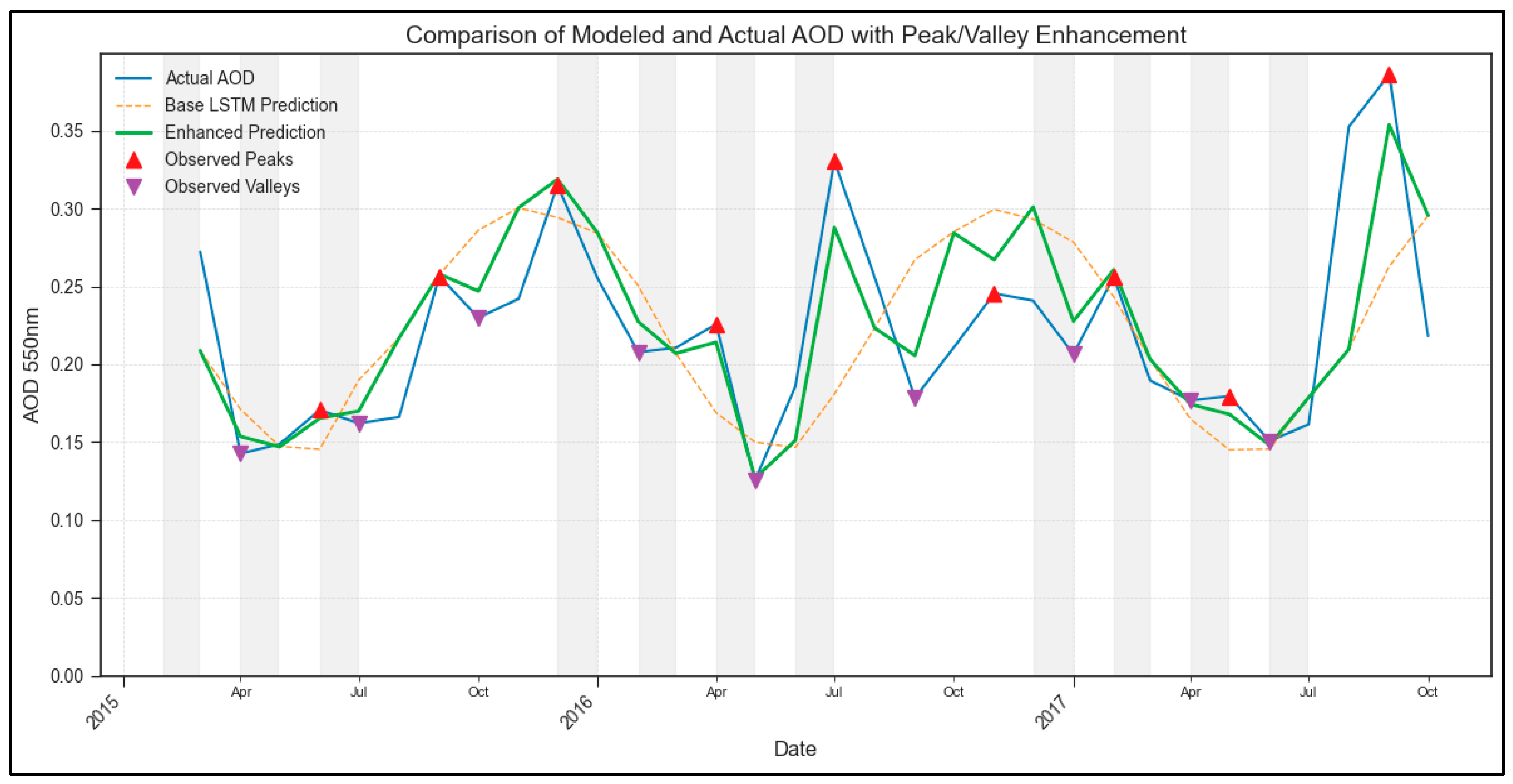
The results demonstrate the capabilities and limitations of using an LSTM model trained on regional data for characterizing AOD dynamics and highlight the specific value of the proposed enhancement methodology. The base LSTM, trained on extended Sicilian data, proved effective at learning the dominant seasonal patterns within its training domain (Figure 2). However, its performance degraded when applied to regions with distinct climatologies and aerosol sources, namely continental Cluj-Napoca (Figure 3) and the maritime Mediterranean (Figure 4), underscoring the strong regional dependence of AOD dynamics and the challenge of model generalization. The base model consistently smoothed high-amplitude peaks and valleys across all regions, a key limitation quantified by the difference between base predictions and observed extrema.

The primary contribution of this work lies in the application and interpretation of the enhanced_peak_valley_amplification post-processing step. While this step incorporates ground-truth information from the period under analysis, rendering it unsuitable for forecasting evaluation, it provides significant value for historical characterization and analysis. Firstly, it serves as a powerful diagnostic tool, quantifying the precise magnitude and timing of the base LSTM’s underestimation of extreme events. Comparing the base and enhanced curves (e.g., in Figure 2 and Figure 4) directly visualizes the model’s structural limitations in representing phenomena such as dust outbreaks or intense pollution episodes. This diagnostic insight is critical for understanding the applicability domains of standard time series models for variables exhibiting such intermittent extremes.

Secondly, the methodology yields an enhanced historical representation (y_enhanced_orig) optimized for subsequent scientific analysis. This hybrid signal merges the model’s learned seasonal baseline with accurately scaled historical peak and valley magnitudes. This product is arguably more valuable than either the noisy raw data or the smoothed base prediction for specific research goals, such as correlating the timing and intensity of accurately represented historical AOD peaks with meteorological drivers, air mass origins, or health impact assessments. The enhancement effectively creates an analysis-ready dataset where key events are represented with higher fidelity. The successful application of this enhancement across diverse regions (land, water, and mixed) demonstrates its robustness as a technique for improving the representation of local extremes, irrespective of the base model’s generalization performance. It is important to consider the influence of cloud contamination on AOD retrievals when interpreting elevated values in the MODIS record. Despite the application of advanced cloud screening algorithms, MODIS retrievals can still be affected by sub-pixel clouds or aerosol–cloud adjacency effects. Thin cirrus or optically thick aerosols may be misclassified, resulting in inflated AOD values. These artifacts are particularly relevant in monthly averaged products, where persistent cloudiness may introduce subtle biases. While our enhancement technique focuses on temporal structure rather than radiative transfer-based corrections, future integration of explicit cloud metrics could improve the interpretability of both the base model and the enhanced outputs.

Though not designed to explicitly correct for cloud-related artifacts, the LSTM model may, in practice, smooth over erratic values when they diverge from expected seasonal patterns. However, without targeted inputs—such as cloud fraction, humidity, or optical thickness—the model lacks the ability to discern genuine aerosol peaks from contaminated retrievals. Future work may explore the integration of such meteorological indicators directly into the training process, allowing the model to identify and de-emphasize likely cloud-induced outliers and further improve the robustness of AOD characterization in persistently cloudy regions.

Comparing the three regions revealed distinct AOD climatologies. Sicily exhibited a Mediterranean pattern with mixed influences. Cluj-Napoca showed stronger seasonality and higher variability typical of a continental site. The Mediterranean Sea displayed a lower baseline dominated by extreme episodic events. The model and enhancement procedure effectively captured these differing characteristics, particularly in the enhanced representations.

The study also acknowledges several limitations that warrant consideration. First, the use of monthly data inevitably smooths out finer temporal variability, potentially masking sub-monthly AOD, which averages out finer temporal details, and the non-predictive nature of the enhancement method. Future work could explore higher temporal resolution data, incorporate meteorological predictors into the LSTM to improve its intrinsic generalization capabilities, investigate more complex deep learning architectures, or perform detailed source attribution for the identified peaks using trajectory models informed by the enhanced AOD time series. Developing true forecasting models that leverage the seasonal and transitional insights gained from this characterization remains a key objective.

5. Conclusions and Future Directions

5.1. Conclusions

This investigation centered on characterizing AOD dynamics utilizing an LSTM network, augmented by a bespoke post-processing methodology. The LSTM model, initially trained on a comprehensive dataset from Sicily spanning over two decades, demonstrated proficiency in capturing the underlying seasonality and general trends inherent within its training domain. However, a notable observation was the model’s inherent tendency to attenuate the magnitude of extreme AOD events, namely sharp peaks and deep valleys, a limitation consistently observed across all test regions.

The application of the trained model to distinct geographical areas—continental Cluj-Napoca and the maritime Central Mediterranean—underscored the challenge of model generalization. Performance naturally varied when confronting AOD regimes differing significantly from the training environment, highlighting the strong regional specificity of aerosol behaviors.

Crucially, the introduced enhanced_peak_valley_amplification post-processing step proved highly effective. While acknowledging its reliance on ground-truth data from the analysis period (rendering it unsuitable for direct forecasting), its utility is twofold. Firstly, it functions as a potent diagnostic tool, precisely quantifying the extent to which the baseline LSTM underestimates or misrepresents extreme AOD occurrences. This offers valuable insight into the structural limitations of standard sequence models when applied to time series marked by intermittent, high-amplitude events. Secondly, and perhaps more significantly for subsequent research, the methodology yields an enhanced historical AOD representation. This refined dataset, effectively merging the model’s grasp of seasonal patterns with accurately scaled historical extrema, presents a more robust basis for specific analytical goals, such as investigating the drivers behind significant aerosol events or assessing their impacts, compared to either the raw, potentially noisy observations or the smoothed baseline model output. The procedure demonstrated robustness across diverse land, mixed, and water regions.

In essence, the combined approach provides a valuable framework not only for modeling AOD but also for critically evaluating model performance concerning extreme events and generating an analysis-ready historical dataset that more faithfully represents the observed atmospheric variability, particularly during high and low AOD episodes.

5.2. Future Work and Directions

Despite the insights gained, certain limitations point toward avenues for future investigation. The reliance on monthly aggregated AOD data inevitably obscures finer temporal details; exploring the application of similar methodologies to higher-resolution datasets (e.g., daily) could reveal sub-monthly dynamics currently averaged out.

To improve the intrinsic predictive power and generalization capabilities of the core model, future iterations could benefit substantially from the incorporation of relevant meteorological predictors (e.g., wind patterns, humidity, boundary layer height) directly into the LSTM architecture. This might allow the model to learn more complex relationships driving AOD variations beyond simple seasonality.

Furthermore, investigating more sophisticated deep learning architectures, potentially hybrid models combining convolutional layers (for spatial context, if applicable) with LSTMs or employing attention mechanisms, could enhance the model’s ability to capture sharp transitions and extreme events without extensive post-processing.

The enhanced AOD time series generated herein, with its accurately represented peaks, offers a prime opportunity for subsequent analysis. Coupling these data with atmospheric back-trajectory models could facilitate more detailed source attribution studies, pinpointing the origins and transport pathways associated with the identified high AOD events.

Finally, while this study focused on historical characterization, a key objective remains the development of genuine AOD forecasting systems. Leveraging the understanding of seasonal patterns, transition periods, and the nature of extreme events gained from this work could inform the design of more accurate and reliable predictive models for future AOD conditions.