A Deep Learning Method for Improving Community Multiscale Air Quality Forecast: Bias Correction, Event Detection, and Temporal Pattern Alignment

Abstract

Accurate air quality forecasting is essential for environmental management and health protection. However, conventional air quality models often exhibit systematic biases and underpredict pollution events due to uncertainties in emissions, meteorology, and atmospheric processes. Addressing these limitations, this study introduces a hybrid deep learning model that integrates convolutional neural networks (CNNs) and Long Short-Term Memory (LSTM) for ozone forecast bias correction. The model is trained here, using data from ten stations in Texas, enabling it to capture both spatial and temporal patterns in atmospheric behavior. Performance evaluation shows notable improvements, with a Root Mean Square Error (RMSE) reduction ranging from 34.11% to 71.63%. F1 scores for peak detection improved by up to 37.38%, Dynamic Time Warping (DTW) distance decreased by 72.77%, the Index of Agreement rose up to 90.09%, and the R² improved by up to 188.80%. A comparison of four loss functions—Mean Square Error (MSE), Huber, Asymmetric Mean Squared Error (AMSE), and Quantile Loss—revealed that MSE offered balanced performance, Huber Loss achieved the highest reduction in systematic RMSE, and AMSE performed best in peak detection. Additionally, four deep learning architectures were evaluated: baseline CNN-LSTM, a hybrid model with attention mechanisms, a transformer-based model, and an End-to-End framework. The hybrid attention-based model consistently outperformed others across metrics while maintaining lower computational demands.

1. Introduction

The Community Multiscale Air Quality (CMAQ), developed by the United States Environmental Protection Agency (EPA), is one of the most extensively used chemical transport models (CTMs) for air pollution forecasting [1,2]. CMAQ is an open-source multi-dimensional model that forecasts air pollutant concentrations (e.g., ozone, particulates, NOx), offering forecasts at fine temporal and geographical resolutions. Due to its versatility, CMAQ has been widely adopted in regional air quality assessments and policymaking. However, its predictive accuracy is constrained by uncertainties in emission inventories, physical and chemical parameterizations, and meteorological inputs, leading to biases in pollutant concentration estimations, particularly for ozone. Chatani et al. [3] demonstrated these limitations when developing a high-resolution 3D regional air quality simulation framework over Japan. Kitayama et al. [4] specifically examined uncertainties in O₃ concentrations simulated by CMAQ using four different chemical mechanisms. Morino et al. [5] evaluated ensemble approaches for improving O₃ and PM_2.5 simulation accuracy. Trieu et al. [6] further highlighted these challenges when evaluating summertime surface ozone in the Kanto area of Japan using a semi-regional model.

To mitigate these limitations, studies have explored pollutant transport modeling and data assimilation techniques, incorporating ground-based observations and remote sensing products to enhance CMAQ’s reliability. Bocquet et al. [7] provided a comprehensive review of data assimilation in atmospheric chemistry models, discussing current status and future prospects. Huang et al. [8] developed a data assimilation method combined with machine learning for anthropogenic emission adjustment in CMAQ. Jung et al. [9] investigated the impact of aerosol optical depth assimilation on meteorology and air quality during the KORUS-AQ campaign. Despite improvements, fundamental uncertainties in atmospheric dynamics persist, limiting even the most advanced assimilation methods. Bessagnet et al. [10] analyzed the effectiveness of data assimilation for air quality forecasting using semi-real case studies. Menut and Bessagnet [11] quantified the expected benefits of data assimilation for air quality forecasting through academic test cases. Rao et al. [12] specifically explored the fundamental limits to the accuracy of regional-scale air quality models. CMAQ’s reliance on bottom-up NOx emissions further complicates ozone simulations, as these emissions are highly variable due to fluctuations in anthropogenic activities and the short atmospheric lifetime of NO₂ [13,14,15]. The discrepancies among multiple emissions inventories exacerbate these challenges, emphasizing the need for improved modeling approaches that account for both meteorological influences and complex atmospheric chemistry.

Machine learning (ML) and deep learning (DL) approaches have emerged as powerful alternatives or complementary methods to traditional numerical models, facilitating efficient multi-hour predictions of atmospheric components based on historical datasets. Biancofiore et al. [16] developed recursive neural network models for the analysis and forecasting of particulate matter. Díaz-Robles et al. [17] created a hybrid AutoRegressive Integrated Moving Average (ARIMA) and artificial neural networks model for urban area particulate matter forecasting in Temuco, Chile. Eslami et al. [18] implemented a real-time hourly ozone prediction system using deep convolutional neural networks. The same research group [19] further developed a data ensemble approach using extremely randomized trees and deep neural networks for real-time air quality forecasting. Lops et al. [20] extended these techniques to create a real-time 7-day forecast of pollen counts using convolutional neural networks. Sayeed [21] integrated deep neural networks with numerical models to improve weather and air quality forecasting across both spatial and temporal dimensions. Hybrid modeling approaches integrate artificial intelligence (AI) techniques with data preprocessing and optimization algorithms. Yuan et al. [22] developed a novel multi-factor and multi-scale method for PM_2.5 forecasting that incorporates decomposition methods. Wang et al. [23] created an innovative hybrid model based on outlier detection and correction algorithms combined with heuristic intelligent optimization for daily air quality index forecasting. Li et al. [24] implemented cluster-based bagging of constrained mixed-effects models for high spatiotemporal resolution nitrogen oxides prediction over large regions. Xu et al. [25] designed an air quality early-warning system for Chinese cities utilizing smart optimization techniques. Deep learning architectures, particularly convolutional neural networks (CNNs) and Long Short-Term Memory (LSTM) networks, have demonstrated significant improvements in air quality forecasting by effectively capturing spatiotemporal patterns in pollutant dispersion. Kim et al. [26] developed a CNN+LSTM hybrid neural network specifically for daily PM_2.5 prediction. Wen et al. [27] designed a novel spatiotemporal convolutional long short-term neural network for air pollution prediction that addresses both spatial and temporal dimensions. Yang et al. [28] created a PM_2.5 prediction model with a novel multi-step-ahead forecasting approach based on dynamic wind field distance. The combination of Graph Neural Networks (GNNs) with LSTMs (GNN-LSTM) has further enhanced predictive performance, reducing root mean square error (RMSE) by up to 40% compared to conventional CTMs, as shown by Borrego et al. [29]. These advancements illustrate the potential of deep learning in refining air quality forecasts by addressing nonlinear dependencies in atmospheric processes.

In addition to hybrid modeling, advanced bias correction techniques have been employed to address systematic errors in air quality models. The use of Kalman filter-based bias correction has been particularly effective in improving forecasts for ozone and PM₁₀. Borrego et al. [29] demonstrated how bias-correction techniques can significantly improve air quality forecasts over Portugal using a Kalman filter approach. June et al. [30] implemented operational bias correction for PM_2.5 using the AIRPACT air quality forecast system in the Pacific Northwest, achieving substantial improvements in forecast accuracy. Similarly, analog bias correction techniques have been successfully applied to NAQFC PM_2.5 predictions, improving the representation of time series trends and diurnal variations as presented by Huang et al. [31]. Other statistical approaches, like Nonhomogeneous Gaussian Regression (NGR) and model-driven data fusion frameworks, have demonstrated their effectiveness in reducing systematic errors and uncertainty in air quality forecasting [32].

Recent studies have further integrated deep learning models with CTMs to enhance predictive accuracy by addressing inherent biases and uncertainties [33,34]. Techniques such as bias correction using machine learning [35], hybrid CNN-LSTM modeling [36], and data-driven emission estimation [37] have significantly improved air pollution forecasting. Additionally, the incorporation of GNNs has enhanced spatial dependency modeling, leading to more precise regional air quality predictions [38]. Furthermore, physics-informed deep neural networks (PINNs) have emerged as an effective approach, integrating fundamental atmospheric chemistry principles within deep learning frameworks [39]. Other studies have explored the use of deep learning for air pollutant emission estimation [40], neural network simulations of CTM outputs [41,42], and post-processing techniques such as CMAQ-CNN [43]. These advancements highlight the transformative potential of AI in improving air quality models by enhancing accuracy, computational efficiency, and real-time adaptability.

Building upon these recent advancements in atmospheric modeling and artificial intelligence, this study introduces a hybrid framework that integrates the WRF-CMAQ modeling system with a deep neural network (DNN) to improve ozone forecasting. By merging physics-based simulations with data-driven learning, the approach seeks to reduce inherent biases in deterministic models and enhance the spatial and temporal accuracy of air quality predictions. The proposed CNN-LSTM architecture is rigorously optimized and benchmarked against alternative deep learning configurations, demonstrating superior performance in terms of error reduction, temporal alignment, and event detection. This work contributes a robust and generalizable methodology that effectively bridges traditional numerical modeling with modern machine learning, offering enhanced predictive reliability and actionable insights for air quality management and policy development.

2. Materials and Methods

This study introduces a hybrid DNN model for bias correction in CMAQ-based ozone (O₃) forecasts. The architecture integrates CNNs and LSTM networks to model both spatial and temporal dependencies critical to air quality prediction. The model was trained using historical O₃ concentration data and meteorological variables collected from ten monitoring stations in Texas, USA. Each station represents distinct atmospheric and pollution conditions. Training was conducted individually for each station to enable localized learning.

2.1. Meteorology—Air Quality Data

For each monitoring station, observed meteorological conditions for the years 2013 and 2014 were obtained from the U.S. Environmental Protection Agency (EPA). Corresponding modeled outputs were also collected from the WRF and CMAQ [44] models within the EQUATES dataset [37]. WRF is a well-established mesoscale weather prediction system, recognized for its ability to simulate local weather and climate dynamics at high spatial resolution. Its output served as a forecasting feature in the DNN model for predicting meteorological conditions on the following day. In parallel, CMAQ provided next-day O₃ concentration predictions. This integrated framework, leveraging WRF and CMAQ, enabled a comprehensive approach to air quality forecasting.

Table 1. Main characteristics of the hourly ozone concentration measurements per station. T stands for temperature.

Station	Lat, Lon	Mean O3 (ppb)	Max O3 (ppb)	Std O3 (ppb)	Mean T (°C)	Max T (°C)	Std T (°C)	Mean Wind Speed (m/s)	Std Wind Speed (m/s)
1	26.54, −97.53	24.3	68.0	12.2	23.0	37.2	6.7	3.3	1.7
2	26.26, −98.24	23.0	69.0	11.3	23.0	40.6	7.4	3.1	1.4
3	27.51, −99.46	23.0	93.0	13.2	23.1	42.0	8.2	3.1	1.6
4	29.02, −95,47	23.9	91.0	14.5	20.3	37.2	7.6	2.4	1.5
5	29.28, −103.20	40.8	71.0	9.9	20.2	39.4	8.6	3.4	1.8
6	29.67, −98.54	29.1	95.0	16.9	18.8	39.0	9.2	2.4	1.4
7	29.74, −93.85	21.3	94.5	15.6	20.0	39.3	8.1	2.0	1.4
8	29.88, −95.33	25.1	79.0	12.7	20.2	36.7	7.8	3.2	1.7
9	29.87, −94.96	23.0	101.0	15.1	19.9	39.4	8.6	2.2	1.5
10	31.52, −104.88	32.3	97.0	15.0	17.5	39.5	10.1	3.5	1.8

summarizes the main characteristics of the hourly ozone concentration measurements dataset for all stations used here, including key statistical properties of ozone concentrations, temperature, and wind speed. All selected monitoring stations maintained excellent data completeness, with each station having more than 90% of valid measurements throughout the study period.

2.2. Data Preprocessing

2.2.1. Missing Data Handling

Missing values in the O₃ time series were imputed using a two-level imputation strategy. Gaps of up to 4 h were filled using linear interpolation, while for longer gaps, historical patterns from the preceding 24 or 48 h were leveraged to reconstruct the time series.

2.2.2. Feature Engineering

The preprocessing stage further encompassed several procedures. Comprehensive feature engineering was implemented to enhance the predictive capabilities of the time-series dataset, including the following:

–

Fourier transformations: Fourier features were introduced to capture periodic fluctuations in the data over different temporal scales (daily, weekly, monthly, and yearly) using sine and cosine components for multiple harmonics of these periods to recognize recurring patterns;

–

Trigonometric time encoding: Hour, day, and month values were sinusoidally transformed to preserve temporal cyclicity;

–

Statistical aggregates: Daily max, min, mean of meteorological and air quality variables, such as temperature, wind speed, CMAQ O₃ predictions, and past station measurements, to provide insights into broader trends;

–

Rolling window features: 4 h moving windows computed local means, extrema, standard deviation, and slope of stations’ measurements to detect sudden changes and emerging trends;

–

Sliding window statistics: The sliding window technique used in this DNN model is a crucial feature engineering method for handling sequential data, such as time series forecasting. By transforming the original dataset into overlapping sequences of fixed-length windows, the model can learn patterns and dependencies over past observations to make future predictions. Specifically, for each sample in the dataset, the input features (X) are structured into windows of size 4, capturing recent trends. This approach helps the model develop a temporal understanding of the data, improving its ability to generalize and make accurate predictions. By applying this technique to both the training and testing sets, the model ensures consistency in feature representation and maintains temporal structure, which is essential for forecasting tasks.

The combination of these features allowed the dataset to capture both long-term seasonal variations and short-term fluctuations, to improve the accuracy of time-series forecasting models. The selection of features was refined iteratively, with features retained or discarded based on their impact on model performance.

2.2.3. Normalization and Data Splitting

Normalization and Scaling: MinMaxScaler was selected for data normalization to scale input features and target variables (O₃ concentrations) to a range of [0, 1], preserving the relative distribution of values while preventing dominance of larger numerical magnitudes. This step was essential for optimizing neural network training by ensuring training stability and preserving the relative magnitudes across variables. While StandardScaler (which standardizes features to a zero mean and unit variance) was evaluated, MinMaxScaler outperformed it, particularly under non-Gaussian distributions.

Data Splitting: The dataset is partitioned into training and validation sets at a 70/30 ratio, preserving temporal integrity. The division is crucial for assessing the model’s performance and its capacity to generalize to unfamiliar data. The validation period spans June–December 2014 to encompass the ozone peak season, due to increased solar radiation and photochemical activity. Capturing this seasonal variability in the validation set is essential for assessing the model’s effectiveness in forecasting high-pollution events, particularly relevant for public health and regulatory applications. The 70/30 split also ensures that the model is trained on a sufficiently large and diverse dataset while reserving an adequately long and representative holdout period for validation.

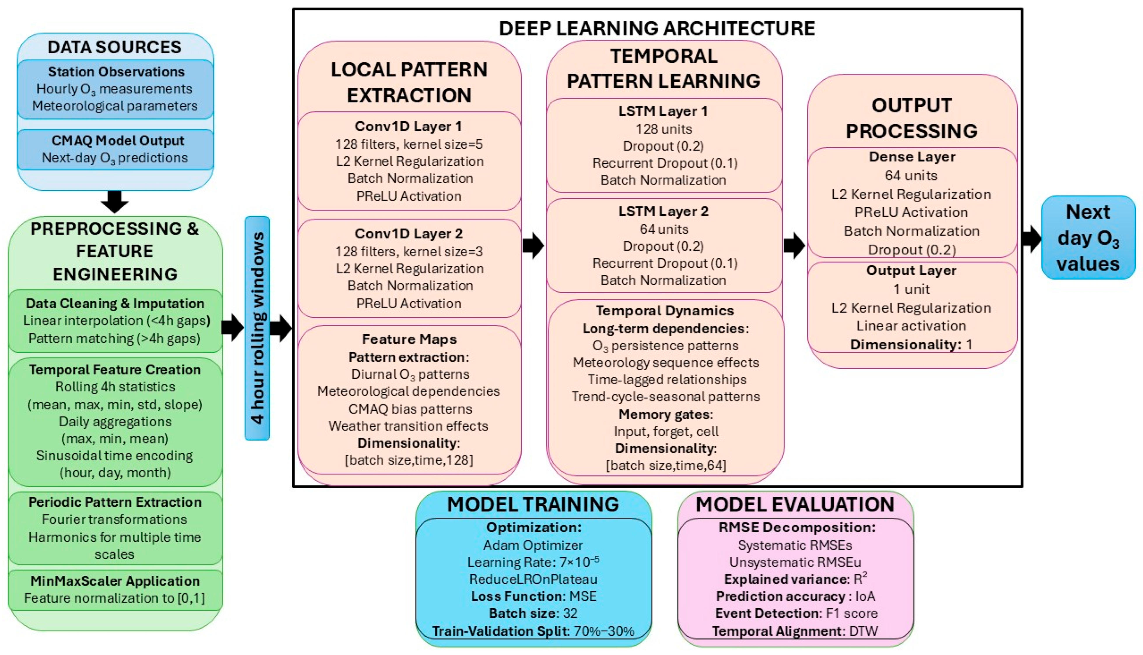
2.3. DNN Model Overview

The forecasting model is based on a hybrid deep neural network integrating Convolutional Neural Networks (CNNs) and Long Short-Term Memory (LSTM) layers to capture both spatial and temporal dependencies within air quality time-series data. This architecture was designed to address the inherent complexity of meteorological and pollutant dynamics, where spatial variations (e.g., across weather and monitoring stations) and temporal sequences (e.g., daily cycles, meteorological lags) influence O₃ concentration patterns.

The model architecture comprises the following key components:

–

Two 1D Convolutional (Conv1D) layers, each followed by batch normalization and Parametric Rectified Linear Unit (PReLU) activations, to extract localized temporal-spatial features from the multivariate input series;

–

Two LSTM layers, stacked sequentially to model long-range temporal dependencies. These are configured to return sequences to preserve timestep continuity and are regularized using dropout and recurrent dropout to mitigate overfitting;

–

A fully connected (dense) layer with L2 regularization and PReLU activation, which integrates high-level representations learned by the LSTM layers;

–

An output layer configured for regression, using the Mean Squared Error (MSE) as the loss function.

This model configuration was selected as the baseline configuration, following a preliminary evaluation of various depth and complexity levels to balance complexity, generalization, and computational efficiency. Section 2.3.1 describes the optimization strategy and hyperparameter tuning procedures used to validate and refine the architecture, including sensitivity analyses over key design choices such as the number of Conv1D and LSTM layers, filter sizes, and unit counts.

2.3.1. Model Optimization and Hyperparameter Tuning

To optimize the deep learning model for bias correction, a systematic sensitivity analysis was conducted to evaluate the influence of key hyperparameters. These included the following:

–

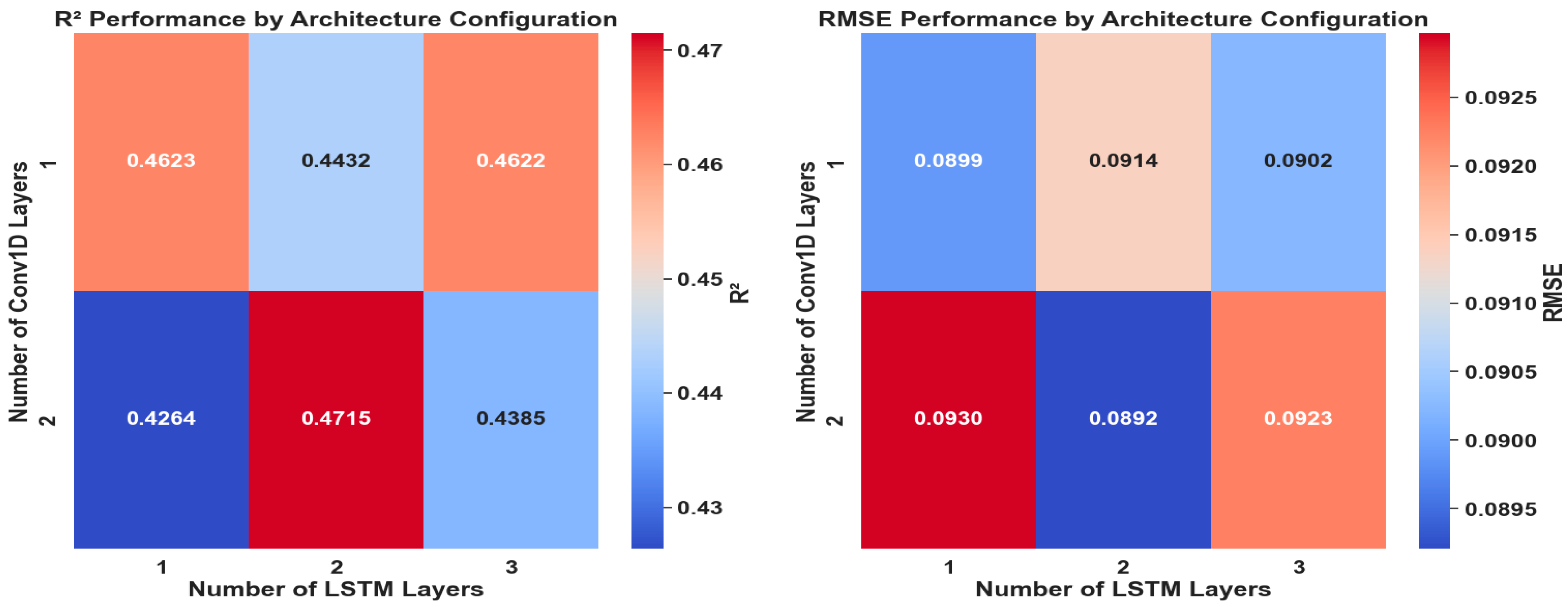
The number of Conv1D and LSTM layers;

–

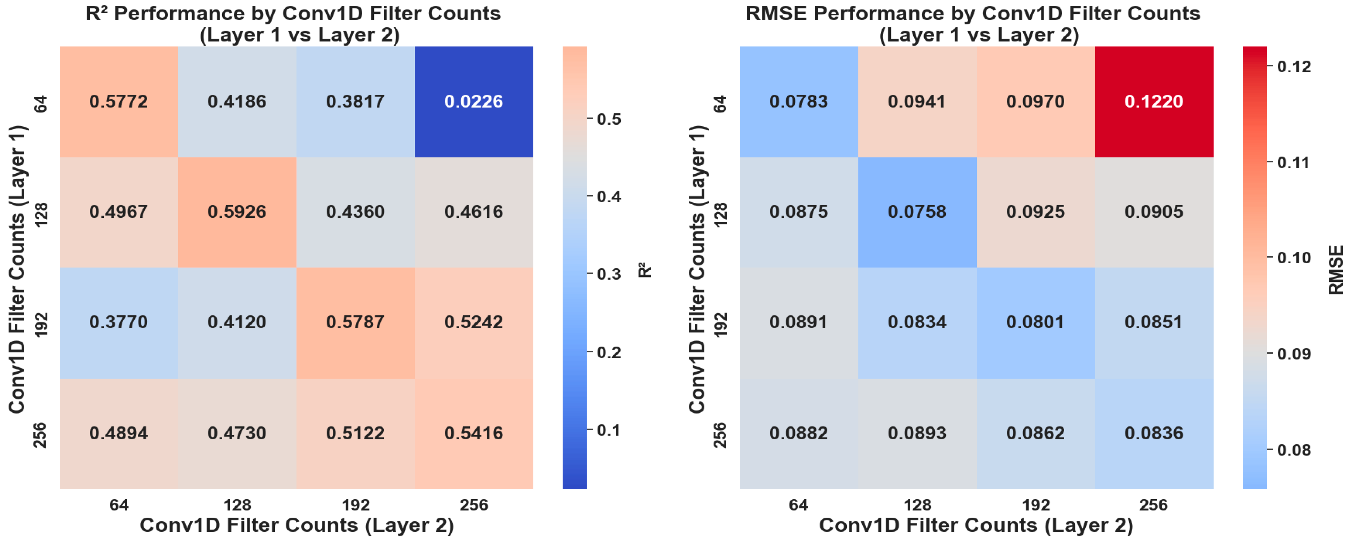
The number of filters per Conv1D layer;

–

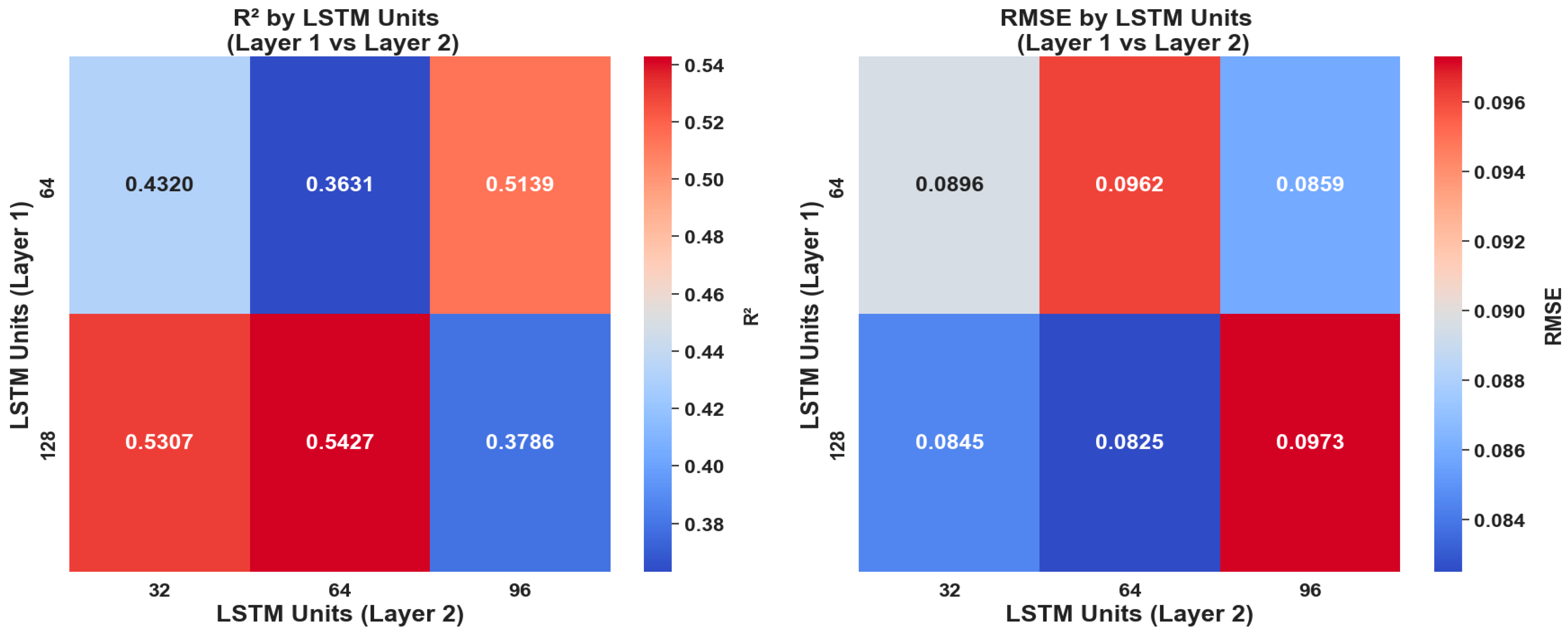
The number of LSTM units per layer.

The goal was to balance model complexity, spatial-temporal feature extraction, and generalization capacity while mitigating overfitting. Various configurations were explored:

–

1–2 Conv1D layers for spatial pattern extraction;

–

1–3 LSTM layers for capturing temporal dependencies;

–

Symmetric and asymmetric filter arrangements in the Conv1D layers (e.g., 64–64, 128–128);

–

Progressive reduction in LSTM units across layers to reflect hierarchical feature refinement.

This analysis contributes to identifying optimal structural characteristics by testing combinations of depth and width in both convolutional and recurrent layers. The rationale for architectural decisions, such as progressively reducing LSTM units, was guided by both theoretical considerations (hierarchical representation learning) and practical efficiency (training stability and parameter reduction).

2.3.2. Model Compilation and Training Strategy

The model is compiled using the Adam optimizer. The Adam optimizer is chosen for its adaptive learning rate adjustments that facilitate efficient optimization in non-stationary deep learning environments. It combines momentum and adaptive learning rate strategies to ensure faster convergence and reduce oscillations during training.

To enhance training efficiency and prevent overfitting, early stopping is employed, terminating training when validation loss stagnates. Additionally, the ReduceLROnPlateau scheduler dynamically adjusts the learning rate when validation loss plateaus, enabling finer optimization by allowing the model to converge more effectively at a slower pace.

A batch size of 32 is used, offering several advantages, particularly in atmospheric time-series forecasting. Smaller batch sizes facilitate more frequent weight updates, accelerating convergence while improving the model’s ability to escape local minima and explore the loss landscape effectively. Moreover, stochastic gradient descent benefits from this level of randomness, mitigating overfitting, especially in complex datasets. In time-series analysis, where capturing fine-grained temporal dependencies is critical, a small batch size preserves data variability within each batch, fostering robust learning even in the presence of noise and non-linearity.

2.4. Performance Metrics

To rigorously evaluate the performance of the developed DNN model, several key statistical metrics were employed. These metrics offer critical insights into the model’s predictive accuracy, robustness, and its ability to capture underlying patterns in the observed data. The chosen metrics encompass both traditional error quantification and specialized measures tailored to time-series analysis and classification performance.

Root Mean Square Error (RMSE) was used as the primary regression metric, reflecting the average magnitude of prediction errors. RMSE penalizes larger errors more heavily than smaller ones, making it particularly useful for assessing regression accuracy. However, RMSE alone does not differentiate between systematic (bias-related) and unsystematic (random) errors. To address this, RMSE was decomposed into systematic (RMSEs) and unsystematic (RMSEu) components. RMSEs capture consistent prediction biases, while RMSEu reflects random variability that is not explained by the model. High RMSEs indicate that the model systematically over- or underestimates values, suggesting calibration issues or structural misspecification. RMSEu, on the other hand, quantifies the random errors in predictions. These errors stem from the model’s inability to fully capture variability in the data due to noise, insufficient training data, or overly complex patterns. Lower RMSEu values indicate a more stable and reliable model in capturing fluctuations without excessive variance. By analyzing RMSEs and RMSEu separately, we gain deeper insights into the model’s performance beyond standard RMSE.

A well-calibrated model should ideally have a low RMSE (indicating minimal bias) while maintaining a relatively small RMSEu (signifying minimal random error). If RMSEs are high, adjustments to the model’s architecture or training strategy may be necessary to reduce systematic bias. Conversely, a high RMSEu might indicate that the model requires better feature engineering, additional training data, or improved regularization to enhance its ability to generalize. This decomposition allows for a more nuanced evaluation of the model’s predictive quality, ensuring that both accuracy and reliability are considered when optimizing its performance.

Another critical metric is the Coefficient of Determination (R²), which measures how well the predictions explain the variance in the observed data, with values close to 1 indicating strong predictive power. The Index of Agreement (IoA) complements R² by quantifying the overall agreement between predicted and observed values.

For event detection (e.g., ozone peaks), the F1 score was used, balancing precision (correctly predicted positives) and recall (correct detection of actual positives), which is particularly useful for imbalanced datasets.

Finally, Dynamic Time Warping (DTW) [45,46] was applied to evaluate temporal alignment between predicted and actual time series, accommodating non-linear shifts in time, a crucial aspect for sequential data.

Table S1 presents the mathematical formulations of these evaluation metrics, providing a comprehensive reference for understanding their computational mechanisms and significance in assessing model performance.

3. Results and Discussion

3.1. Sensitivity Analysis of Model Architecture

To optimize the model configuration, a sensitivity analysis on the number of Conv1D and LSTM layers was performed. Conv1D layers are essential for capturing spatial patterns in time-series data. We evaluated configurations with one or two such layers to determine whether adding an additional convolutional layer would meaningfully improve feature extraction. LSTM layers are responsible for modeling temporal dependencies. We assessed architectures with up to three LSTM layers to evaluate the impact of increased depth on predictive performance. While increasing the number of LSTM layers may improve temporal representation, it also increases computational complexity and the risk of overfitting. Therefore, the combination of 1–2 Conv1D and 1–3 LSTM layers offered a comprehensive range to investigate the model’s performance and identify the optimal balance between spatial and temporal modeling capabilities.

Figure 1 shows the relationship between the number of Conv1D and LSTM layers and the model’s performance, measured in terms of R² and RMSE. The left heatmap, depicting R² values, clearly demonstrates that the optimal configuration is achieved with 2 Conv1D layers and 2 LSTM layers, yielding the highest R² value of approximately 0.4715. This finding indicates that the specific combination most effectively captures the underlying temporal and spatial patterns in the data. Conversely, configurations with only 1 Conv1D layer exhibited relatively lower R² values, suggesting that a single convolutional layer is insufficient to fully extract spatial features. The right heatmap, showing RMSE values, corroborates this observation as the lowest RMSE (0.0892) is also obtained with the same configuration of 2 Conv1D and 2 LSTM layers, indicating superior prediction accuracy.

It is worth noting that increasing the number of LSTM layers to 3 tends to slightly degrade performance across both metrics, likely due to overfitting and increased model complexity. Similarly, configurations with just one Conv1D layer generally exhibited higher RMSE values, further emphasizing the necessity of a more substantial convolutional foundation. Overall, these results indicate that the optimal architectural balance between convolutional and recurrent components involves employing 2 Conv1D layers followed by 2 LSTM layers. This configuration enables efficient feature extraction while preserving robust temporal modeling, ultimately enhancing the model’s ability to perform accurate bias correction.

To choose the most effective combination of Conv1D filters, the sensitivity analysis shown in Figure 2 analyzes the impact of the number of filters in each Conv1D layer on model performance. It is evident that the combination of 128 filters in the first Conv1D layer and 128 filters in the second Conv1D layer achieved finer predictive performance.

This indicates that intermediate complexity (128–128) achieves a beneficial balance between capturing sufficient information and maintaining generalization capability. Also, it is observed that using the same number of filters in both Conv1D layers generally yields good results. In contrast, asymmetrical configurations tend to exhibit a wider range of performances, with some combinations underperforming significantly.

In designing the LSTM architecture, the decision to progressively reduce the number of units across consecutive LSTM layers is rooted in both theoretical principles and practical considerations. The first LSTM layer, typically containing a higher number of units, is responsible for capturing broad and complex temporal patterns within the data, as it directly processes the raw input. These patterns often contain long-term dependencies that require substantial representational capacity. However, as the information propagates through the network, the subsequent layers focus on more refined and localized temporal relationships. Reducing the number of units in these deeper layers helps the model concentrate on distilling and fine-tuning the features already learned, without overburdening the model with excessive complexity.

This architectural choice also addresses overfitting concerns, as maintaining a consistently high number of units across all layers increases the risk of memorization rather than generalization. Furthermore, reducing the number of units results in fewer parameters, making the model more computationally efficient and faster to train while still maintaining performance. This progressive reduction mirrors the way hierarchical information processing occurs, transitioning from coarse to fine-grained features, ultimately improving model robustness and generalizability.

The impact of varying LSTM unit configurations on model performance is illustrated in Figure 3. Increasing the number of units in the first LSTM layer from 64 to 128 significantly enhances predictive accuracy, as evidenced by higher R² values and lower RMSE. Specifically, the combination of 128 units in the first layer and 64 units in the second layer achieves the best results. This configuration demonstrates the importance of assigning a relatively higher capacity to the initial LSTM layer to capture the primary temporal dependencies, while the subsequent layer can afford to have fewer units to fine-tune the information.

3.2. Sensitivity Analysis of Loss Functions

The model concludes with an output layer that directly predicts ozone concentrations, with particular attention given to the choice of loss function. A comprehensive sensitivity analysis (Supplementary Materials, Figures S1–S8), across four loss functions—Mean Squared Error (MSE), Asymmetric Mean Squared Error (AMSE), Quantile Loss, and Huber Loss—revealed distinct performance characteristics. MSE delivered balanced performance across metrics, serving as a reliable baseline. Huber Loss, however, achieved the highest reduction in RMSE at several stations (up to 72.03% improvement over CMAQ) and was especially effective in correcting systematic error, with RMSEs reduced by up to 98.88% at Station 4. AMSE excelled in peak event detection, yielding F1 Score improvements of up to 50.69% at Station 2, making it particularly valuable for identifying high-pollution episodes. The Quantile Loss, while not consistently outperforming other functions, offered competitive temporal alignment as measured by DTW at certain stations.

This multi-loss function strategy enables targeted optimization based on specific forecasting priorities, whether reducing bias, improving peak detection, or minimizing overall error. By combining CNNs for spatial feature extraction with LSTMs for temporal sequence modeling, and selecting loss functions tailored to distinct objectives, the model effectively captures the complex dynamics of air quality. This integrated approach leads to significant improvements in forecast accuracy, robustness, and operational relevance across a broad range of evaluation metrics.

3.3. Final Neural Network Architecture

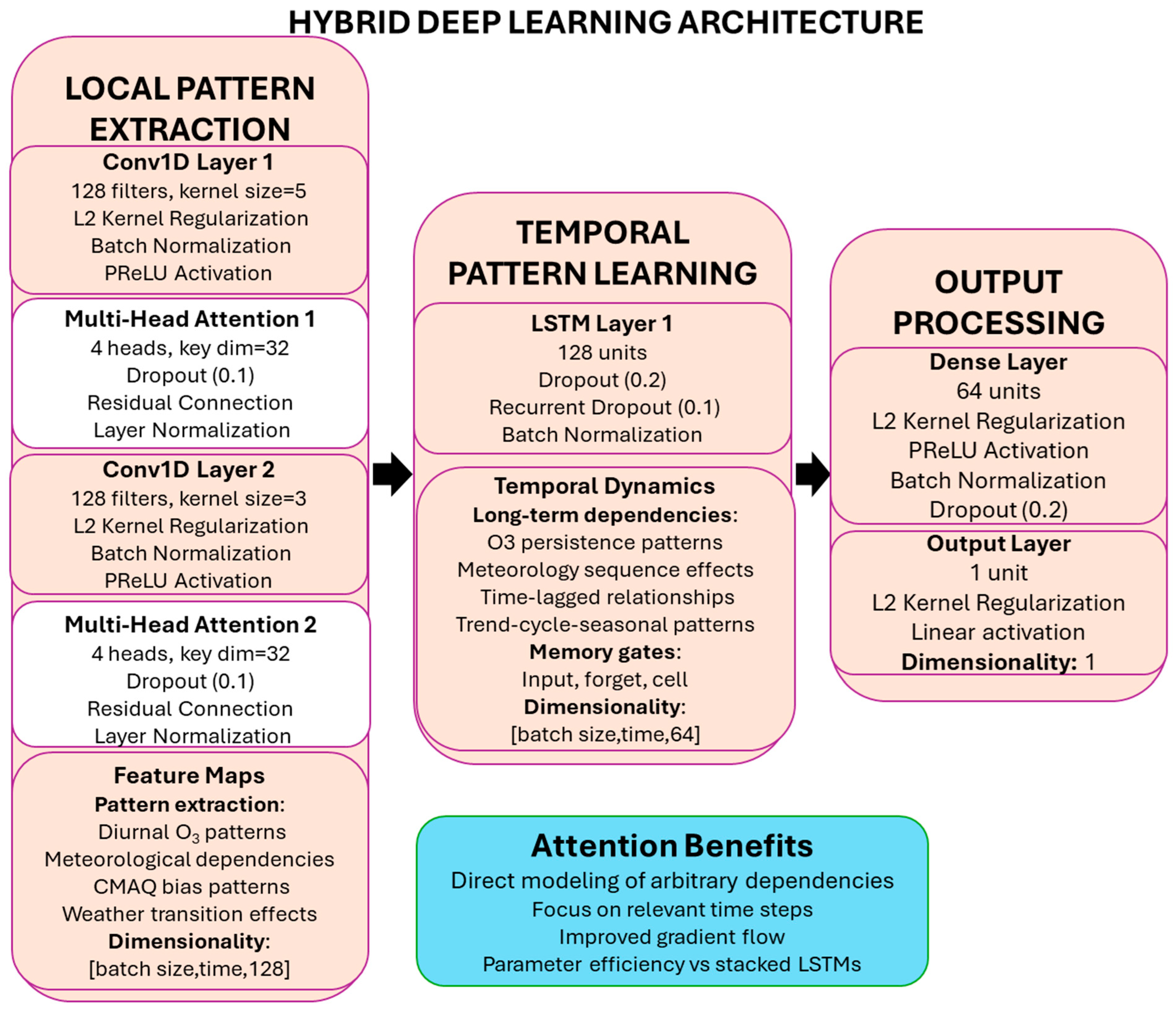
Figure 4 presents the network architecture of the DNN model used in this study, along with a description of each layer and all input features incorporated into this comprehensive schematic. The diagram illustrates how various data inputs, including meteorological forecasts, current observations, and temporal encodings, flow through the hybrid CNN-LSTM architecture to produce bias-corrected O₃ predictions.

The architecture begins with two sequential Conv1D layers, each with 128 filters. These layers are designed to extract localized temporal features from the input sequences and are followed by batch normalization layers to stabilize and accelerate training. PReLU activation functions are applied to introduce learnable non-linearities, allowing the network to adaptively model both positive and negative trends in the data.

To reduce overfitting and improve generalization, dropout layers are incorporated after the convolutional and recurrent stages. A dropout rate of 0.2 is used to balance training stability with robustness. Batch normalization is applied consistently across the network to standardize activations and improve convergence behavior.

The extracted convolutional features are subsequently passed through two stacked LSTM layers with 128 and 64 units, respectively. These LSTM layers are configured to return sequences, preserving temporal dependencies between timesteps and allowing the model to capture complex, long-range temporal relationships. Regularization is applied through both standard dropout and recurrent dropout mechanisms, effectively mitigating the risk of overfitting by randomly disabling neurons during training. Each LSTM layer is followed by batch normalization to maintain stable gradients and ensure efficient learning.

Following the LSTM layers, a fully connected dense layer with 64 neurons is employed to integrate high-level features extracted from the recurrent layers. This dense layer incorporates L2 kernel regularization to penalize excessive weight magnitudes, further enhancing generalization. PReLU activation continues to maintain adaptive learning, while a final batch normalization and dropout layer consolidate the network’s robustness.

The model concludes with an output layer that directly predicts the Mean Squared Error (MSE), serving as the loss function. This choice ensures precise regression predictions by heavily penalizing larger errors. By integrating CNNs for spatial pattern recognition and LSTMs for capturing temporal dependencies, the model adeptly manages the complex dynamics of air quality forecasting, achieving improved accuracy and robustness.

In summary, the finalized architecture includes the following:

–

Two Conv1D layers (128 filters each, PReLU activation, batch normalization, dropout rate = 0.2);

–

Two LSTM layers (128 and 64 units, both returning sequences, with batch normalization and recurrent dropout);

–

One dense layer (64 neurons, L2 regularization, PReLU, batch normalization, and dropout);

–

Output layer with MSE loss function.

3.4. Alternative Data Splits and Robustness Check

To evaluate the robustness of model performance, additional train/validation splits (60/40 and 80/20) and train/validation/test splits (60/20/20, 70/15/15, and 80/10/10) were used in a sensitivity analysis. The results, detailed in the Supplementary Materials (Tables S2–S7, Figures S9–S17), show that the 70/30 split used in the main analysis consistently achieves strong performance across key metrics, particularly for RMSE, F1 score, DTW, and IoA. While the 60/20/20 split demonstrated slightly higher average performance in some cases, especially in systematic error correction and temporal alignment, the 70/30 split offers the best balance between model learning capacity and evaluation reliability. These findings confirm that the model’s effectiveness is stable across varying partition strategies and validate the selection of the 70/30 split for both methodological soundness and seasonal representativeness.

3.5. Performance Metrics Results

The results concerning the RMSE, along with its systematic and unsystematic components for each station, are presented in

Table 2. RMSE improvement.

Station	RMSE			RMSES			RMSEU
	Model	CMAQ	Improvement	Model	CMAQ	Improvement	Model	CMAQ	Improvement
1	7.75	22.87	66.11%	0.548	19.42	97.18%	7.73	12.09	36.06%
2	7.15	25.20	71.63%	0.80	21.25	96.23%	7.10	13.54	47.54%
3	7.97	26.67	70.11%	0.68	22.90	97.02%	7.94	13.66	41.88%
4	8.67	23.93	63.91%	0.42	19.67	97.88%	8.63	13.63	36.70%
5	6.38	14.41	55.72%	0.374	10.22	96.34%	6.37	10.16	37.29%
6	9.75	21.61	54.86%	1.17	16.90	93.07%	9.68	13.47	28.09%
7	8.75	21.95	60.13%	2.23	17.92	87.54%	8.46	12.69	33.29%
8	8.05	22.64	64.46%	0.26	18.83	98.64%	8.04	12.58	36.07%
9	8.55	21.15	59.55%	0.13	16.99	99.26%	8.55	12.59	32.06%
10	8.43	12.79	34.11%	1.45	7.08	79.56%	8.30	10.66	22.07%

.

The AI model significantly outperforms the original CMAQ model predictions across all monitoring stations, with RMSE reduction ranging from 34.11% to 71.63%. Notably, the most substantial improvement is observed at station 2, where the RMSE is reduced from 25.20 ppb to 7.15 ppb, yielding a 71.63% improvement. The lowest improvement is seen at station 10, where RMSE drops from 12.79 ppb to 8.43 ppb, corresponding to a 34.11% improvement. These results indicate that the AI model consistently reduces the overall prediction error, regardless of spatial variability among stations. The improvements suggest that the model effectively captures local patterns and temporal fluctuations that the original CMAQ model fails to address.

Regarding systematic error correction, the AI model exhibits remarkable performance in mitigating consistent biases, achieving RMSE reductions between 79.56% and 99.26%. The most significant reduction is observed at station 9, where the RMSEs drop from 16.99 ppb to 0.13 ppb, translating to a 99.26% improvement. Similarly, station 4 shows an RMSE decrease from 19.67 ppb to 0.42 ppb, achieving a 97.88% improvement. The lowest improvement occurs at station 10, where RMSEs decrease from 7.08 ppb to 1.45 ppb, corresponding to a 79.56% improvement. The substantial improvements in RMSEs across all stations highlight the AI model’s efficiency in correcting systematic biases, which are often linked to structural deficiencies in the CMAQ model or its inability to capture localized meteorological and emission variations.

The AI model also demonstrates notable improvements in RMSEu, which quantifies the random error, thereby reflecting its ability to address variability that does not follow consistent patterns. RMSEu reductions range from 22.07% to 47.54%, with the highest decrease at station 2, where RMSEu drops from 13.54 ppb to 7.10 ppb (47.54% improvement). The lowest improvement is at station 10, where RMSEu decreases from 10.66 ppb to 8.30 ppb, yielding a 22.07% improvement. Other stations, such as 23,178 (33.29%) and 4 (36.70%), also display substantial improvements, suggesting that the AI model efficiently minimizes random fluctuations. While the improvements in RMSEu are not as pronounced as those in RMSEs, they still demonstrate the AI model’s ability to capture unpredictable patterns and noise. This distinction is important, as reducing RMSEu is inherently more challenging due to the presence of residual uncertainties and random errors stemming from complex atmospheric processes.

The consistent and significant reductions in both RMSEs and RMSEu indicate that the AI model not only effectively corrects systematic biases but also reduces random errors, reinforcing the robustness of the bias correction methodology. This dual improvement improves predictive accuracy by aligning forecasts more closely with observed values while stabilizing fluctuations and variability. Moreover, the fact that RMSE reductions surpass RMSEu reductions across all stations suggests that the model primarily addresses systematic biases while achieving reasonable improvements in random error reduction. This outcome highlights the challenge of accurately predicting random atmospheric variability while also demonstrating that the model’s structural enhancements significantly mitigate recurring bias issues.

The results further indicate that station-specific characteristics play a critical role in the model’s performance. Stations such as 2 and 3, where the original CMAQ model exhibited substantial errors, benefit the most from the bias correction, achieving improvements exceeding 70%. Conversely, stations like 10 and 9 show lower improvements, likely due to inherently unpredictable local conditions or limited data variability. This spatial heterogeneity emphasizes the need for adaptive models that are capable of accounting for location-specific meteorological and environmental dynamics. Fine-tuning the model for each station or introducing regional calibration techniques could further enhance performance. Figure 5 shows the RMSE results for each station.

The model’s ability to accurately predict peak events, temporal alignment, overall agreement with observations, and variance explanation is presented in

Table 3. F1 score, DTW, IoA, and R² improvement.

Station	F1 Score			DTW			IoA			R2
	Model	CMAQ	Improvement (%)	Model	CMAQ	Improvement (%)	Model	CMAQ	Improvement (%)	Model	CMAQ	Improvement (%)
1	0.61	0.45	35.30	2.98	8.15	63.47	0.81	0.43	90.09	0.42	−4.09	110.16
2	0.59	0.43	37.38	2.68	9.84	72.77	0.84	0.42	99.76	0.47	−5.61	108.34
3	0.70	0.60	16.37	3.31	10.36	68.05	0.87	0.47	84.60	0.56	−3.96	114.05
4	0.51	0.48	5.91	3.59	8.82	59.31	0.88	0.51	72.68	0.59	−2.14	127.60
5	0.63	0.56	14.56	2.13	5.12	58.34	0.83	0.54	54.28	0.51	−1.51	133.62
6	0.80	0.70	13.60	4.31	10.40	58.58	0.91	0.65	39.31	0.65	−0.70	188.80
7	0.68	0.67	0.79	3.69	9.14	59.59	0.91	0.66	38.20	0.65	−1.22	152.84
8	0.65	0.52	25.82	3.31	8.24	59.76	0.86	0.53	61.64	0.56	−2.51	122.13
9	0.65	0.63	2.67	3.52	9.67	63.60	0.90	0.64	41.63	0.63	−1.26	149.94
10	0.80	0.78	2.34	3.63	5.38	32.62	0.92	0.84	10.04	0.70	0.32	122.70

.

In the context of bias correction and air quality modeling, a high F1 score indicates accurate detection of high pollution events (peaks), which are critical for public health decision-making. The AI model outperforms CMAQ across all monitoring stations, with F1 score improvements ranging from 0.79% to 37.38%. The most significant enhancement is observed at station 2, where the F1 score increases from 0.43 to 0.59, yielding a 37.38% improvement. In contrast, the smallest improvement is observed at station 7 with an F1 increase from 0.67 to 0.68 (0.79%), indicating that the original CMAQ model already had relatively high peak detection accuracy at this station. Moderate improvements are seen at stations like 5 (14.56%) and 10 (2.34%), suggesting that the AI model’s peak prediction accuracy varies with station characteristics and data distribution. These improvements reflect the AI model’s enhanced ability to detect pollution peaks, thereby making it more reliable for warning systems and high pollution event predictions.

In addition to peak detection, the AI model significantly enhances the alignment between predicted and actual time series, as indicated by reductions in DTW distance compared to the CMAQ model. The DTW improvements range from 32.62% to 72.77%, highlighting the AI model’s superior ability to capture temporal pollution dynamics. The highest improvement is seen at station 2, where DTW decreases from 9.84 to 2.68, corresponding to an improvement of 72.77%. Station 3 also shows substantial improvement, with DTW dropping from 10.36 to 3.31, yielding an improvement of 68.05%. The lowest improvement is at station 10, where DTW reduces from 5.38 to 3.63 (32.62%). These significant DTW reductions across most stations indicate that the AI model aligns predicted pollution levels more closely with observed values, an essential factor for real-time monitoring and forecasting.

Overall, the improvements in both peak detection and temporal alignment underscore the AI model’s effectiveness in addressing key limitations of the CMAQ model, particularly in high pollution event forecasting. The results of these enhancements are presented in Figure 6.

As far as evaluating the degree of model prediction error relative to the observed variance, the AI model significantly improves the IoA across all monitoring stations, with improvements ranging from 10.04% to 90.09%. The most substantial improvement occurs at station 1, where the IoA increases from 0.43 to 0.81, representing a 90.09% increase, while the lowest is observed at station 10, where the IoA rises from 0.84 to 0.92 (10.04%). Notably, at station 3, the CMAQ model exhibits a negative IoA value (−3.962), indicating severe prediction errors or a fundamental inability to capture the observed variability. The AI model effectively corrects this issue, achieving a significantly improved IoA of 0.87. The consistently high improvements in the IoA demonstrate that the AI model not only reduces the magnitude of prediction errors but also significantly enhances the alignment of predicted values with the actual data distribution, reflecting its robust calibration and error-correction capabilities.

Finally, when assessing how much of the variance in the observed data is captured by the model, the AI model achieves remarkable improvements in R², ranging from 110.16% to 188.80%. The most substantial improvement is noted at station 6, where R² increases from −0.65 to 0.91, resulting in an improvement of 188.80%. Similarly, station 1 shows an R² rise from −4.09 to 0.42, yielding a 110.16% improvement. Even at station 10, where the CMAQ model initially performs well, R² improves from 0.84 to 0.92 (22.70%), demonstrating that the AI model further refines prediction accuracy.

The improvements in R² indicate that the bias correction model not only mitigates systematic errors but also significantly enhances the model’s ability to capture variance in the actual observations. This translates into more accurate and consistent predictions across diverse monitoring stations. The IoA and R² results are also presented in Figure 7. Figures S18–S27 in the Supplementary present comparative time series visualizations for each station.

3.6. Attention-Based Enhancements and Model Intercomparison

Attention mechanisms have emerged as a powerful component in deep learning architectures, initially developed for natural language processing but now widely applied in time series forecasting. Unlike traditional sequence models that process all input elements equally, attention mechanisms dynamically focus on relevant parts of the input sequence when generating predictions. In the context of air quality forecasting, attention mechanisms offer several advantages:

• The ability to identify and prioritize the most relevant time steps for prediction;
• Improved handling of long-range dependencies in temporal data;
• Enhanced interpretability by providing insight into which inputs most influence the prediction.

3.6.1. Hybrid CNN-LSTM with Attention Enhancement

The hybrid architecture developed here integrates multi-head self-attention mechanisms with CNN and LSTM components to enhance the model’s ability to capture complex temporal dependencies in air quality data. The hybrid model maintains the CNN-LSTM backbone while incorporating transformer-style attention mechanisms, creating a synergy between feature engineering and modern deep learning techniques. Figure 8 illustrates the architecture.

The incorporation of multi-head self-attention mechanisms allowed the reduction of model complexity by removing one LSTM layer while maintaining—or in many cases improving—forecast performance. This architectural decision aligns with the principle of parameter efficiency, as attention mechanisms effectively model both short-term and long-range temporal dependencies with fewer parameters than stacked recurrent layers, as introduced by Vaswani et al. [47]. By replacing the second LSTM layer with attention, the resulting hybrid model achieves improved or comparable results across key evaluation metrics. Specifically, across ten monitoring stations, the hybrid model outperformed the original CNN-LSTM in several critical areas. Notably, the hybrid model achieved higher F1 score improvements at station 6 (38.84%) and station 9 (64.20%), demonstrating superior capability in detecting high ozone events, an essential aspect for air quality warning systems. The hybrid model also produced higher or comparable improvements in RMSE at stations 2, 3, 4, and 10, and consistently matched or exceeded CNN-LSTM performance in systematic error correction (RMSEs), with 99.47% at station 4 and 99.34% at station 8. Furthermore, improvements in temporal alignment (DTW) were marginally higher with the attention-based model at stations 3, 7, and 9, confirming that the architecture preserved the model’s ability to learn fine-grained temporal dynamics. The model also maintained high agreement with observed data (IoA), with performance exceeding 97% at several stations. Beyond performance, the use of attention mechanisms provides computational advantages. While LSTM layers process sequentially, attention operations are highly parallelizable, reducing training time and enabling more efficient deployment in operational forecasting systems. This efficiency is particularly important in air quality applications, where models require regular retraining as new monitoring data becomes available. The comparative evaluation, illustrated in Figure 9, confirms that the attention-enhanced hybrid model not only reduces architectural complexity but also improves practical applicability without sacrificing modeling capacity.

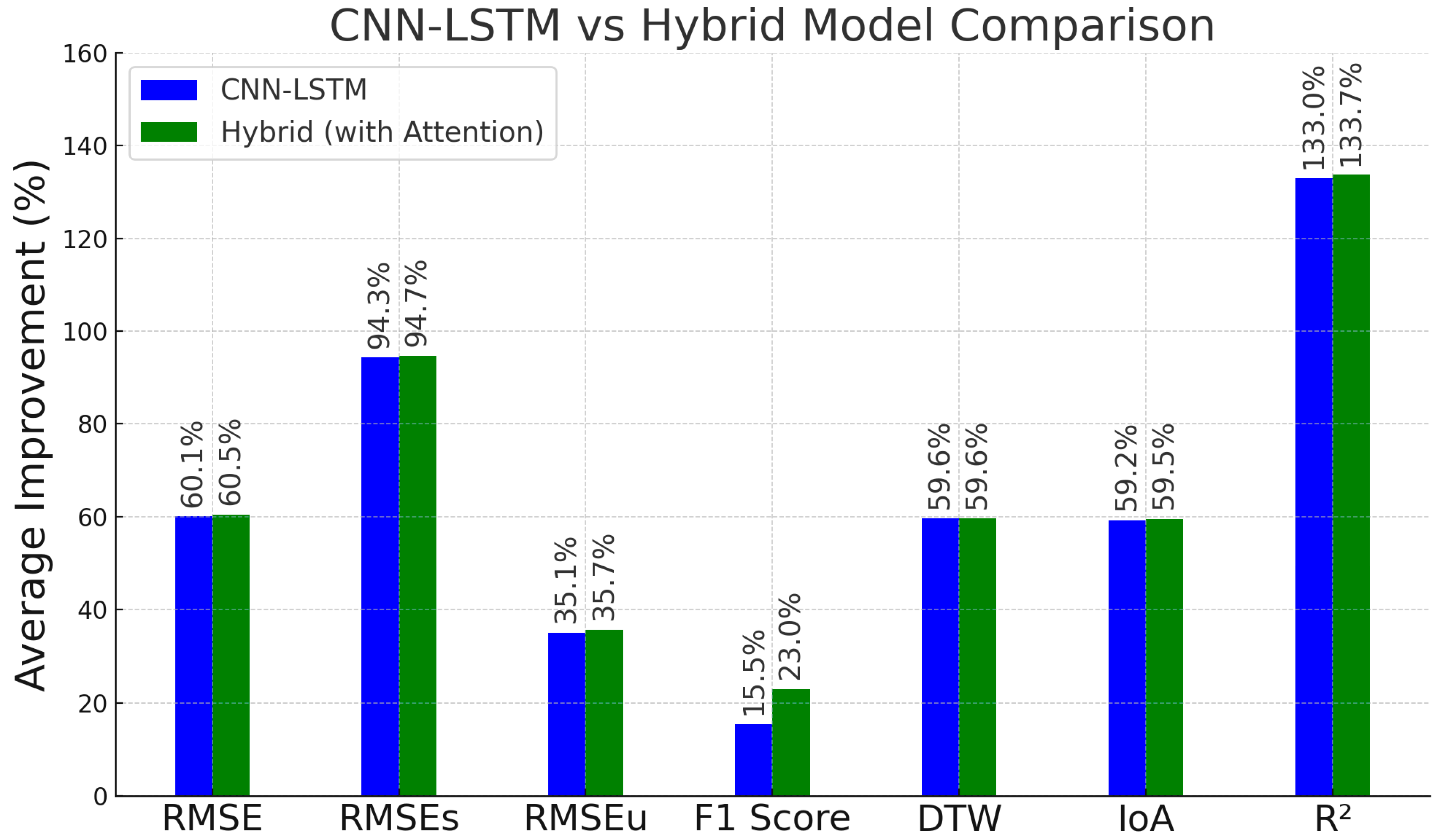
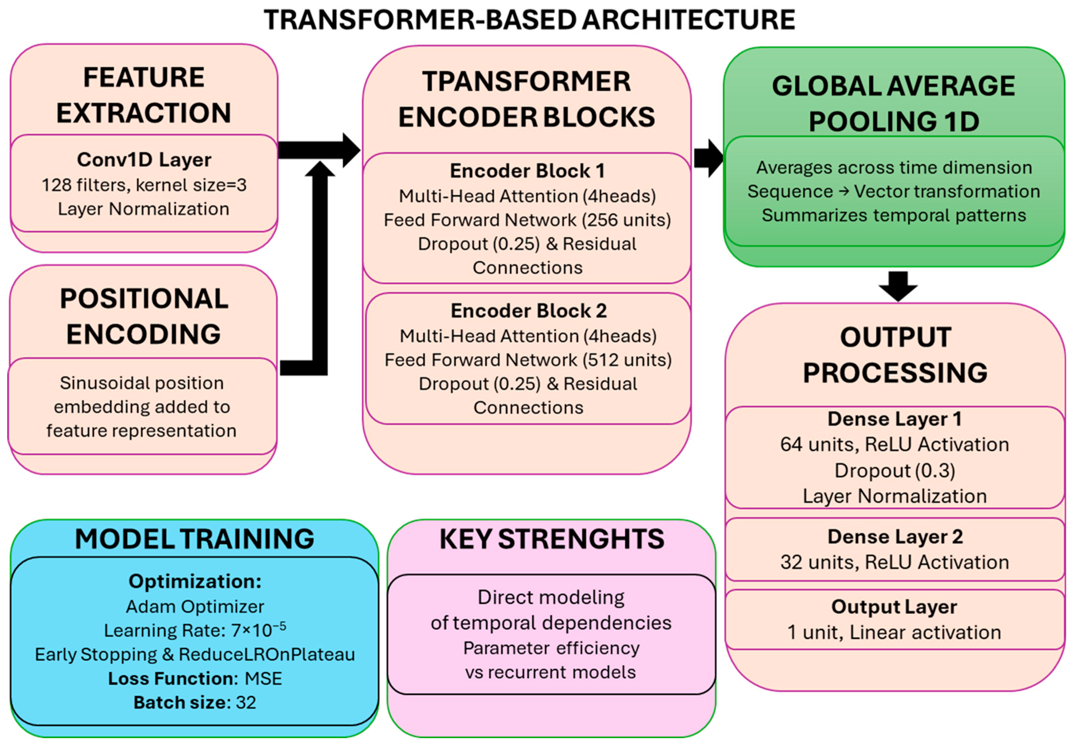
3.6.2. Comparison of Deep Learning Approaches for Air Quality Forecasting

In addition to the Hybrid CNN-LSTM model with attention mechanisms, the study explored two modern deep learning architectures to assess their suitability for air quality forecasting tasks: a pure transformer-based model and an End-to-End learning approach (Figure 10 and Figure 11). The transformer-based model (Figure 10) leverages the self-attention mechanism, which enables direct modeling of dependencies between arbitrary positions in the input sequence. This architecture consists of a convolutional feature extraction layer, sinusoidal positional encoding, and two transformer encoder blocks with varying attention heads (4 and 8 heads, respectively). The model employs multi-head self-attention to capture complex temporal relationships in air quality data without relying on recurrent connections. This approach offers theoretical advantages in handling long-range dependencies and parallel computation compared to traditional recurrent architectures. The End-to-End learning approach (Figure 11) represents a more radical departure from conventional methods by minimizing domain-specific feature engineering. This model employs a multi-resolution feature extraction block with parallel convolutional layers of different kernel sizes (1, 3, and 5) to capture patterns at multiple time scales. Positional information is learned through a dense layer rather than using fixed embeddings. Two transformer encoder blocks with increasing capacity (2 to 4 attention heads) process the combined features, followed by a sophisticated prediction network with residual connections. This architecture exemplifies the modern paradigm of letting the model automatically discover relevant features directly from raw data.

Performance evaluation across multiple metrics revealed that while both modern architectures demonstrated competitive capabilities, neither consistently outperformed the Hybrid model (Figure 12). The transformer-based approach showed particular strength in F1 score improvement, outperforming all other models at stations 2, 6, and 9, highlighting its effectiveness in peak pollution event detection, a critical need for early warning systems. However, this is accompanied by increased computational complexity and less consistent improvements in RMSE and RMSEu. The Hybrid model, which integrates attention mechanisms with domain-aware feature inputs, achieved the highest or near-highest performance across RMSE, RMSEs, and DTW in most stations, reflecting its strong bias correction ability and precise temporal alignment. It also delivered more stable improvements across stations, indicating better generalizability. In contrast, the End-to-End model, which omits feature engineering and sequential layers, consistently underperformed, particularly in RMSEu and IoA, underscoring the limitations of generic architectures when applied to complex, domain-sensitive forecasting tasks. These findings suggest that while modern architectural innovations like transformers offer valuable capabilities, particularly for handling long-range dependencies and event detection, domain-specific feature engineering and hybrid architectures continue to provide essential advantages in specialized applications like air quality forecasting. The intercomparison results reinforce the conclusion that hybrid models, which combine structured environmental insight with advanced deep learning methods, currently offer the most effective and efficient solution for this task. Detailed intercomparison results are presented in Tables S8–S13 and Figures S28–S35.

4. Conclusions

The study presented a hybrid deep learning model that significantly improves air quality forecasting by correcting systematic biases in CMAQ ozone predictions. The proposed AI-based bias correction model significantly outperformed the CMAQ model across all key statistical metrics, offering both methodological innovation and practical utility for air quality forecasting. Furthermore, an enhanced Hybrid model with attention mechanisms was introduced to improve parameter efficiency and temporal learning, delivering comparable or superior performance to the original CNN-LSTM while reducing model complexity.

The key contributions and findings of this study are summarized below:

• RMSE Decomposition: This study introduced the decomposition of RMSE into its systematic (RMSEs) and unsystematic (RMSEu) components to distinguish model bias from random variability;
• Error Reduction: RMSE was reduced by 34.11% to 71.63% across all monitoring stations;
• Systematic Bias Correction: RMSEs were reduced by up to 99.26%, effectively addressing persistent biases in CMAQ outputs;
• Variability Capture: RMSEu was reduced by up to 47.54%, improving model performance under fluctuating environmental conditions;
• Peak Detection: The F1 score showed significant improvement in peak pollution event detection, with gains of up to 37%, enhancing early warning capabilities for high pollution episodes;
• Temporal Alignment: Dynamic Time Warping (DTW) distance was reduced by up to 72.77%, indicating better alignment with observed temporal patterns;
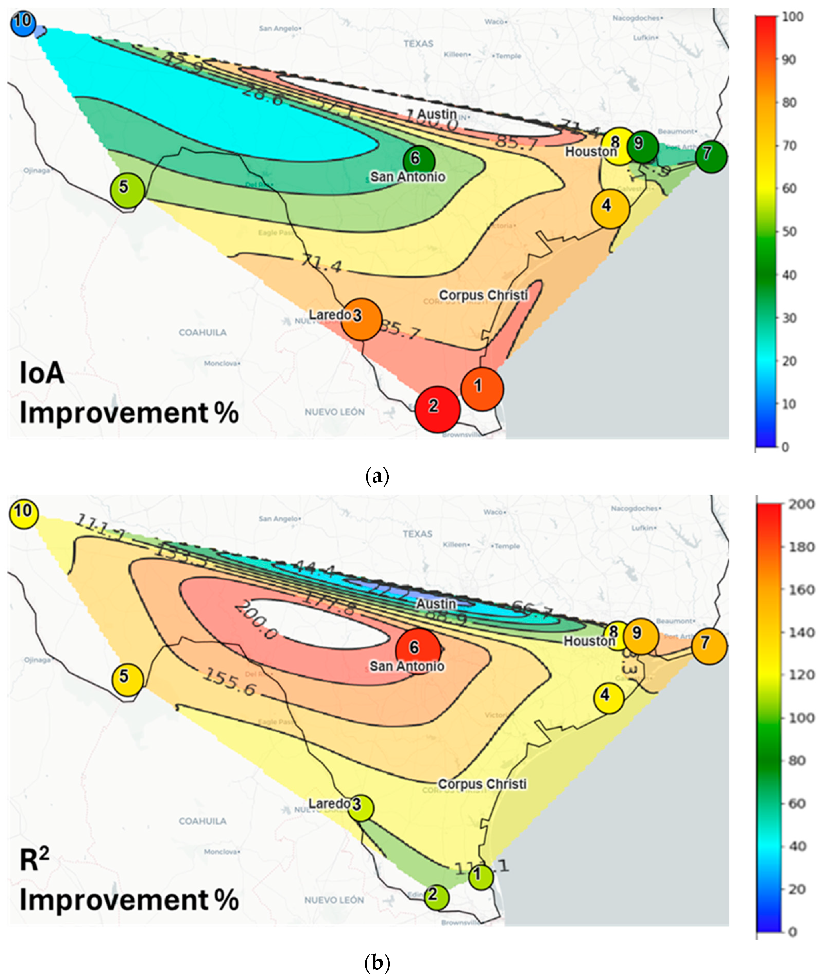
• Model Agreement: The Index of Agreement (IoA) improved by up to 90.09%, confirming better overall predictive accuracy;
• Explained Variance: The Coefficient of Determination (R²) increased by up to 188.80%, demonstrating a superior ability to capture variability in air quality data;
• Hybrid Architecture Efficiency: The addition of multi-head self-attention mechanisms allowed the removal of one LSTM layer, maintaining or improving performance while reducing training time and increasing parallelizability.

This study also demonstrated that the strategic selection of loss functions plays a critical role in optimizing deep learning models for air quality forecasting. By tailoring loss functions to specific objectives, such as bias correction, peak detection, or temporal alignment, the hybrid CNN-LSTM model achieved substantial improvements across multiple evaluation metrics. These findings highlight the importance of aligning model architecture and training objectives with targeted forecasting priorities to enhance predictive performance and operational utility.

The intercomparison study across four architectures—CNN-LSTM, Hybrid with attention, transformer, and End-to-End DNN—confirmed the Hybrid model’s robustness and superior balance across all metrics. While the transformer model excelled in F1 score and event detection at specific stations, and the End-to-End model was computationally efficient, the Hybrid model consistently delivered strong performance in bias correction (RMSEs), temporal synchronization (DTW), and variance explanation (R²), making it the most effective and adaptable solution among the evaluated models. These results validate the model’s effectiveness for air quality forecasting. The consistent performance across diverse metrics and stations demonstrates its practical applicability for real-time monitoring and public health decision-making. The evaluation affirms the potential of this AI approach to advance air quality prediction capabilities, supporting its integration into operational systems. The significant reduction in systematic bias achieved by the proposed deep learning model has important implications for real-world air quality forecasting. Bias correction strengthens the reliability of numerical air quality models, reducing persistent under- or overestimations of pollutant concentrations. This improvement is particularly crucial for regulatory agencies and policymakers relying on accurate forecasts to implement air quality management strategies. Moreover, the improvement in the F1 score enhances early-warning systems for pollution episodes, enabling better public health advisories. Future work could focus on integrating the bias-corrected forecasts into operational air quality models, assessing their impact on policy decisions, and exposure assessments.

It should be pointed out here that although the model was trained and validated using data from monitoring stations located solely in Texas, USA, the underlying approach can be adapted to other geographic regions by retraining on local datasets. Future work will focus on expanding the model’s applicability through retraining with international datasets and incorporating domain adaptation techniques to improve generalization in areas with limited monitoring infrastructure.

A promising direction involves the development of a spatial Deep Neural Network (DNN) that extends CMAQ functionality across diverse geographic regions, regardless of observation station presence. Such an approach would leverage information from neighboring areas and incorporate advanced interpolation techniques where observational data are sparse. By integrating spatial features, such as topography, land use, and meteorological patterns, into the DNN architecture, the model could generalize better in unmonitored regions. Techniques such as Graph Neural Networks (GNNs) or spatial convolution layers could further enhance the ability to capture complex spatial dependencies. This would significantly expand the reach of bias correction, making it valuable for large-scale air quality assessment in regions with limited monitoring infrastructure.

Despite the improvements demonstrated, deep learning models present inherent challenges. Chief among them is the risk of overfitting, especially with limited or region-specific data. Although dropout regularization and batch normalization help mitigate this risk, ongoing validation on unseen data remains essential. Additionally, the data-dependence of these models requires careful consideration when applying them to new geographies or under novel meteorological conditions. Continued model refinement and the integration of adaptive AI techniques will be key to ensuring long-term generalization and operational robustness.

In summary, this study establishes a strong foundation for AI-driven bias correction in air quality modeling. It highlights not only the value of integrating machine learning with domain expertise but also demonstrates the scalability of such approaches through architectural improvements and comparative benchmarking. The resulting framework offers a promising path toward reliable, real-time environmental forecasting systems that support evidence-based public health and policy decisions.

References

1. Appel, K.W.; Bash, J.O.; Fahey, K.M.; Foley, K.M.; Gilliam, R.C.; Hogrefe, C.; Hutzell, W.T.; Kang, D.; Mathur, R.; Murphy, B.N.; et al. The Community Multiscale Air Quality (CMAQ) Model Versions 5.3 and 5.3.1: System Updates and Evaluation. Geosci. Model Dev. 2021, 14, 2867–2897. [Google Scholar] [CrossRef] [PubMed]
2. Byun, D.; Schere, K.L. Review of the Governing Equations, Computational Algorithms, and Other Components of the Models-3 Community Multiscale Air Quality (CMAQ) Modeling System. Appl. Mech. Rev. 2006, 59, 51–77. [Google Scholar] [CrossRef]
3. Chatani, S.; Morikawa, T.; Nakatsuka, S.; Matsunaga, S.; Minoura, H. Development of a Framework for a High-Resolution, Three-Dimensional Regional Air Quality Simulation and Its Application to Predicting Future Air Quality over Japan. Atmos. Environ. 2011, 45, 1383–1393. [Google Scholar] [CrossRef]
4. Kitayama, K.; Morino, Y.; Yamaji, K.; Chatani, S. Uncertainties in O3 Concentrations Simulated by CMAQ over Japan Using Four Chemical Mechanisms. Atmos. Environ. 2019, 198, 448–462. [Google Scholar] [CrossRef]
5. Morino, Y.; Chatani, S.; Hayami, H.; Sasaki, K.; Mori, Y.; Morikawa, T.; Ohara, T.; Hasegawa, S.; Kobayashi, S. Evaluation of Ensemble Approach for O3 and PM2.5 Simulation. Asian J. Atmos. Environ. 2010, 4, 150–156. [Google Scholar] [CrossRef]
6. Trieu, T.T.N.; Goto, D.; Yashiro, H.; Murata, R.; Sudo, K.; Tomita, H.; Satoh, M.; Nakajima, T. Evaluation of Summertime Surface Ozone in Kanto Area of Japan Using a Semi-Regional Model and Observation. Atmos. Environ. 2017, 153, 163–181. [Google Scholar] [CrossRef]
7. Bocquet, M.; Elbern, H.; Eskes, H.; Hirtl, M.; Žabkar, R.; Carmichael, G.R.; Flemming, J.; Inness, A.; Pagowski, M.; Pérez Camaño, J.L.; et al. Data Assimilation in Atmospheric Chemistry Models: Current Status and Future Prospects for Coupled Chemistry Meteorology Models. Atmos. Chem. Phys. 2015, 15, 5325–5358. [Google Scholar] [CrossRef]
8. Huang, C.; Niu, T.; Wu, H.; Qu, Y.; Wang, T.; Li, M.; Li, R.; Liu, H. A Data Assimilation Method Combined with Machine Learning and Its Application to Anthropogenic Emission Adjustment in CMAQ. Remote Sens. 2023, 15, 1711. [Google Scholar] [CrossRef]
9. Jung, J.; Souri, A.H.; Wong, D.C.; Lee, S.; Jeon, W.; Kim, J.; Choi, Y. The Impact of the Direct Effect of Aerosols on Meteorology and Air Quality Using Aerosol Optical Depth Assimilation During the KORUS-AQ Campaign. J. Geophys. Res. Atmos. 2019, 124, 8303–8319. [Google Scholar] [CrossRef]
10. Bessagnet, B.; Menut, L.; Couvidat, F.; Meleux, F.; Siour, G.; Mailler, S. What Can We Expect from Data Assimilation for Air Quality Forecast? Part II: Analysis with a Semi-Real Case. J. Atmos. Ocean. Technol. 2019, 36, 1433–1448. [Google Scholar] [CrossRef]
11. Menut, L.; Bessagnet, B. What Can We Expect from Data Assimilation for Air Quality Forecast? Part I: Quantification with Academic Test Cases. J. Atmos. Ocean. Technol. 2019, 36, 269–279. [Google Scholar] [CrossRef]
12. Rao, S.T.; Luo, H.; Astitha, M.; Hogrefe, C.; Garcia, V.; Mathur, R. On the Limit to the Accuracy of Regional-Scale Air Quality Models. Atmos. Chem. Phys. 2020, 20, 1627–1639. [Google Scholar] [CrossRef] [PubMed]
13. Choi, Y.; Souri, A.H. Chemical Condition and Surface Ozone in Large Cities of Texas during the Last Decade: Observational Evidence from OMI, CAMS, and Model Analysis. Remote Sens. Environ. 2015, 168, 90–101. [Google Scholar] [CrossRef]
14. Li, X.; Choi, Y.; Czader, B.; Roy, A.; Kim, H.; Lefer, B.; Pan, S. The Impact of Observation Nudging on Simulated Meteorology and Ozone Concentrations during DISCOVER-AQ 2013 Texas Campaign. Atmos. Chem. Phys. 2016, 16, 3127–3144. [Google Scholar] [CrossRef]
15. Martin, R.V.; Fiore, A.M.; Van Donkelaar, A. Space-Based Diagnosis of Surface Ozone Sensitivity to Anthropogenic Emissions. Geophys. Res. Lett. 2004, 31, L06120. [Google Scholar] [CrossRef]
16. Biancofiore, F.; Busilacchio, M.; Verdecchia, M.; Tomassetti, B.; Aruffo, E.; Bianco, S.; Di Tommaso, S.; Colangeli, C.; Rosatelli, G.; Di Carlo, P. Recursive Neural Network Model for Analysis and Forecast of PM10 and PM2.5. Atmos. Pollut. Res. 2017, 8, 652–659. [Google Scholar] [CrossRef]
17. Díaz-Robles, L.A.; Ortega, J.C.; Fu, J.S.; Reed, G.D.; Chow, J.C.; Watson, J.G.; Moncada-Herrera, J.A. A Hybrid ARIMA and Artificial Neural Networks Model to Forecast Particulate Matter in Urban Areas: The Case of Temuco, Chile. Atmos. Environ. 2008, 42, 8331–8340. [Google Scholar] [CrossRef]
18. Eslami, E.; Choi, Y.; Lops, Y.; Sayeed, A. A Real-Time Hourly Ozone Prediction System Using Deep Convolutional Neural Network. Neural Comput. Appl. 2020, 32, 8783–8797. [Google Scholar] [CrossRef]
19. Eslami, E.; Salman, A.K.; Choi, Y.; Sayeed, A.; Lops, Y. A Data Ensemble Approach for Real-Time Air Quality Forecasting Using Extremely Randomized Trees and Deep Neural Networks. Neural Comput. Appl. 2020, 32, 7563–7579. [Google Scholar] [CrossRef]
20. Lops, Y.; Choi, Y.; Eslami, E.; Sayeed, A. Real-Time 7-Day Forecast of Pollen Counts Using a Deep Convolutional Neural Network. Neural Comput. Appl. 2020, 32, 11827–11836. [Google Scholar] [CrossRef]
21. Sayeed, A. Integrating Deep Neural Network with Numerical Models to Have Better Weather and Air Quality Forecast Both Spatially and Temporally. Ph.D. Thesis, Department of Earth and Atmospheric Sciences, College of Natural Sciences and Mathematics, University of Houston, Houston, TX, USA, 2021. [Google Scholar]
22. Yuan, W.; Wang, K.; Bo, X.; Tang, L.; Wu, J. A Novel Multi-Factor & Multi-Scale Method for PM2.5 Concentration Forecasting. Environ. Pollut. 2019, 255, 113187. [Google Scholar] [CrossRef] [PubMed]
23. Wang, J.; Du, P.; Hao, Y.; Ma, X.; Niu, T.; Yang, W. An Innovative Hybrid Model Based on Outlier Detection and Correction Algorithm and Heuristic Intelligent Optimization Algorithm for Daily Air Quality Index Forecasting. J. Environ. Manag. 2020, 255, 109855. [Google Scholar] [CrossRef]
24. Li, L.; Girguis, M.; Lurmann, F.; Wu, J.; Urman, R.; Rappaport, E.; Ritz, B.; Franklin, M.; Breton, C.; Gilliland, F.; et al. Cluster-Based Bagging of Constrained Mixed-Effects Models for High Spatiotemporal Resolution Nitrogen Oxides Prediction over Large Regions. Environ. Int. 2019, 128, 310–323. [Google Scholar] [CrossRef] [PubMed]
25. Xu, Y.; Yang, W.; Wang, J. Air Quality Early-Warning System for Cities in China. Atmos. Environ. 2017, 148, 239–257. [Google Scholar] [CrossRef]
26. Kim, H.S.; Han, K.M.; Yu, J.; Kim, J.; Kim, K.; Kim, H. Development of a CNN+LSTM Hybrid Neural Network for Daily PM2.5 Prediction. Atmosphere 2022, 13, 2124. [Google Scholar] [CrossRef]
27. Wen, C.; Liu, S.; Yao, X.; Peng, L.; Li, X.; Hu, Y.; Chi, T. A Novel Spatiotemporal Convolutional Long Short-Term Neural Network for Air Pollution Prediction. Sci. Total Environ. 2019, 654, 1091–1099. [Google Scholar] [CrossRef]
28. Yang, M.; Fan, H.; Zhao, K. PM2.5 Prediction with a Novel Multi-Step-Ahead Forecasting Model Based on Dynamic Wind Field Distance. Int. J. Environ. Res. Public Health 2019, 16, 4482. [Google Scholar] [CrossRef]
29. Borrego, C.; Monteiro, A.; Pay, M.T.; Ribeiro, I.; Miranda, A.I.; Basart, S.; Baldasano, J.M. How Bias-Correction Can Improve Air Quality Forecasts over Portugal. Atmos. Environ. 2011, 45, 6629–6641. [Google Scholar] [CrossRef]
30. June, N.; Vaughan, J.; Lee, Y.; Lamb, B.K. Operational Bias Correction for PM2.5 Using the AIRPACT Air Quality Forecast System in the Pacific Northwest. J. Air Waste Manag. Assoc. 2021, 71, 515–527. [Google Scholar] [CrossRef]
31. Huang, J.; McQueen, J.; Wilczak, J.; Djalalova, I.; Stajner, I.; Shafran, P.; Allured, D.; Lee, P.; Pan, L.; Tong, D.; et al. Improving NOAA NAQFC PM2.5 Predictions with a Bias Correction Approach. Weather. Forecast. 2017, 32, 407–421. [Google Scholar] [CrossRef]
32. Fei, H.; Wu, X.; Luo, C. A Model-Driven and Data-Driven Fusion Framework for Accurate Air Quality Prediction. arXiv 2019, arXiv:1912.07367. [Google Scholar] [CrossRef]
33. Sayeed, A.; Lops, Y.; Choi, Y.; Jung, J.; Salman, A.K. Bias Correcting and Extending the PM Forecast by CMAQ up to 7 Days Using Deep Convolutional Neural Networks. Atmos. Environ. 2021, 253, 118376. [Google Scholar] [CrossRef]
34. Sayeed, A.; Choi, Y.; Eslami, E.; Jung, J.; Lops, Y.; Salman, A.K.; Lee, J.-B.; Park, H.-J.; Choi, M.-H. A Novel CMAQ-CNN Hybrid Model to Forecast Hourly Surface-Ozone Concentrations 14 Days in Advance. Sci. Rep. 2021, 11, 10891. [Google Scholar] [CrossRef]
35. Koo, Y.-S.; Choi, Y.; Ho, C. Air Quality Forecasting Using Big Data and Machine Learning Algorithms. Asia-Pac. J. Atmos. Sci. 2023, 59, 529–530. [Google Scholar] [CrossRef]
36. Bessagnet, B.; Beauchamp, M.; Menut, L.; Fablet, R.; Pisoni, E.; Thunis, P. Deep Learning Techniques Applied to Super-Resolution Chemistry Transport Modeling for Operational Uses. Environ. Res. Commun. 2021, 3, 085001. [Google Scholar] [CrossRef]
37. Fang, L.; Jin, J.; Segers, A.; Liao, H.; Li, K.; Xu, B.; Han, W.; Pang, M.; Lin, H.X. A Gridded Air Quality Forecast through Fusing Site-Available Machine Learning Predictions from RFSML v1.0 and Chemical Transport Model Results from GEOS-Chem V13.1.0 Using the Ensemble Kalman Filter. Geosci. Model Dev. 2023, 16, 4867–4882. [Google Scholar] [CrossRef]
38. Li, L.; Wang, J.; Franklin, M.; Yin, Q.; Wu, J.; Camps-Valls, G.; Zhu, Z.; Wang, C.; Ge, Y.; Reichstein, M. Improving Air Quality Assessment Using Physics-Inspired Deep Graph Learning. npj Clim. Atmos. Sci. 2023, 6, 152. [Google Scholar] [CrossRef]
39. Sharma, H.; Shrivastava, M.; Singh, B. Physics Informed Deep Neural Network Embedded in a Chemical Transport Model for the Amazon Rainforest. npj Clim. Atmos. Sci. 2023, 6, 28. [Google Scholar] [CrossRef]
40. Huang, L.; Liu, S.; Yang, Z.; Xing, J.; Zhang, J.; Bian, J.; Li, S.; Sahu, S.K.; Wang, S.; Liu, T.-Y. Exploring Deep Learning for Air Pollutant Emission Estimation. Geosci. Model Dev. 2021, 14, 4641–4654. [Google Scholar] [CrossRef]
41. Vlasenko, A.; Matthias, V.; Callies, U. Simulation of Chemical Transport Model Estimates by Means of a Neural Network Using Meteorological Data. Atmos. Environ. 2021, 254, 118236. [Google Scholar] [CrossRef]
42. Kow, P.-Y.; Chang, L.-C.; Lin, C.-Y.; Chou, C.C.-K.; Chang, F.-J. Deep Neural Networks for Spatiotemporal PM2.5 Forecasts Based on Atmospheric Chemical Transport Model Output and Monitoring Data. Environ. Pollut. 2022, 306, 119348. [Google Scholar] [CrossRef] [PubMed]
43. Sayeed, A.; Eslami, E.; Lops, Y.; Choi, Y. CMAQ-CNN: A New-Generation of Post-Processing Techniques for Chemical Transport Models Using Deep Neural Networks. Atmos. Environ. 2022, 273, 118961. [Google Scholar] [CrossRef]
44. Skamarock, W.C.; Klemp, J.B.; Dudhia, J.; Gill, D.O.; Barker, D.M.; Duda, M.G.; Huang, X.-Y.; Wang, W.; Powers, J.G. A Description of the Advanced Research WRF Version 4; National Center for Atmospheric Research (NCAR): Boulder, CO, USA, 2019. [Google Scholar] [CrossRef]
45. Berndt, D.J.; Clifford, J. Using Dynamic Time Warping to Find Patterns in Time Series. In Proceedings of the 3rd International Conference on Knowledge Discovery and Data Mining, Seattle, WA, USA, 31 July–1 August 1994; pp. 359–370. [Google Scholar]
46. Vaughan, N.; Gabrys, B. Comparing and Combining Time Series Trajectories Using Dynamic Time Warping. Procedia Comput. Sci. 2016, 96, 465–474. [Google Scholar] [CrossRef]
47. Vaswani, A.; Shazeer, N.; Parmar, N.; Uszkoreit, J.; Jones, L.; Gomez, A.N.; Kaiser, Ł.; Polosukhin, I. Attention Is All You Need. In Proceedings of the 31st International Conference on Neural Information Processing Systems, Long Beach, CA, USA, 4–9 December 2017; Guyon, I., Luxburg, U.V., Bengio, S., Wallach, H., Fergus, R., Vishwanathan, S., Garnett, R., Eds.; Curran Associates, Inc.: Red Hook, NY, USA, 2017; Volume 30, pp. 6000–6010, ISBN 978-1-5108-6096-4. [Google Scholar]
Figure 1. Number of Conv1D and LSTM layers sensitivity analysis.
Atmosphere 16 00739 g001
Figure 2. Number of Conv1D layers, filter count, and sensitivity analysis.
Atmosphere 16 00739 g002
Figure 3. Number of LSTM layers units’ sensitivity analysis.
Atmosphere 16 00739 g003
Figure 4. Architecture of the proposed deep learning model (DNN) for bias correction. The model integrates Conv1D layers for feature extraction and LSTM layers for sequential learning, followed by fully connected layers for prediction.
Atmosphere 16 00739 g004
Figure 5. % Improvement in (a) RMSE, (b) RMSEs, and (c) RMSEu. Numbers in circles indicate the station numbers corresponding to Table 2.
Atmosphere 16 00739 g005
Figure 6. % Improvement in (a) F1 score and (b) DTW. Numbers in circles indicate the station numbers corresponding to Table 2.
Atmosphere 16 00739 g006
Figure 7. % Improvement in (a) IoA, (b) R2. Numbers in circles indicate the station numbers corresponding to Table 2.
Atmosphere 16 00739 g007
Figure 8. Hybrid CNN-LSTM with attention mechanisms architecture.
Atmosphere 16 00739 g008
Figure 9. Average performance comparison between the CNN-LSTM model and the Hybrid model with attention mechanisms.
Atmosphere 16 00739 g009
Figure 10. Transformer-based model architecture.
Atmosphere 16 00739 g010
Figure 11. End-to-End learning architecture.
Atmosphere 16 00739 g011
Figure 12. Average performance comparison across different architectures.
Atmosphere 16 00739 g012