


Application of Machine Learning Algorithms in Nitrous Oxide (N2O) Emission Estimation in Data-Sparse Agricultural Landscapes


Abstract
1. Introduction
2. Materials and Methods
2.1. Data
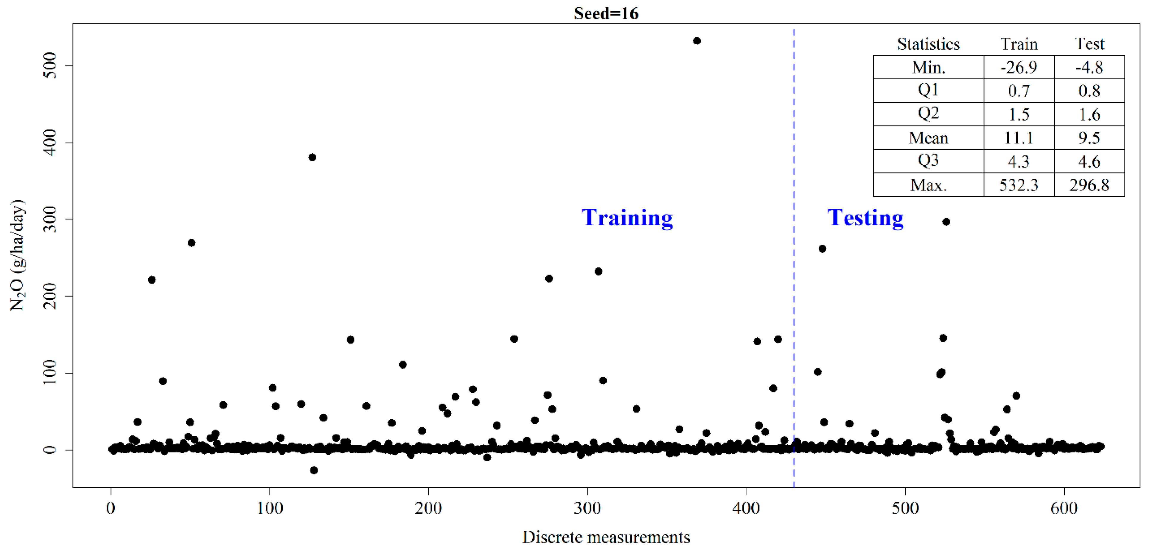
2.2. Training and Testing Data Sampling
2.3. Multiple Linear Regression (MLR)
- (1)
- HILMo: N2O is influenced by all independent predictors of Table 1. There is no interaction among the independent predictors.
- (2)
- HILM: N2O is influenced by all independent predictors of Table 1. There is interaction among ST, VM, Ph and NO3.
- (3)
- LILMo: N2O is influenced by independent variables under LI. No Ph, NO3 or NH4 data values are used to train the model. There is no interaction among the independent predictors.
- (4)
- LILM: N2O is influenced by independent variables under LI. Interaction among the ST, VM and Srain2D was permitted.
2.4. Random Forest Regression (RFR)
2.5. Support Vector Regression (SVR)
2.6. Artifical Neural Networks (ANNs)
2.7. Comparison Metrics
3. Results
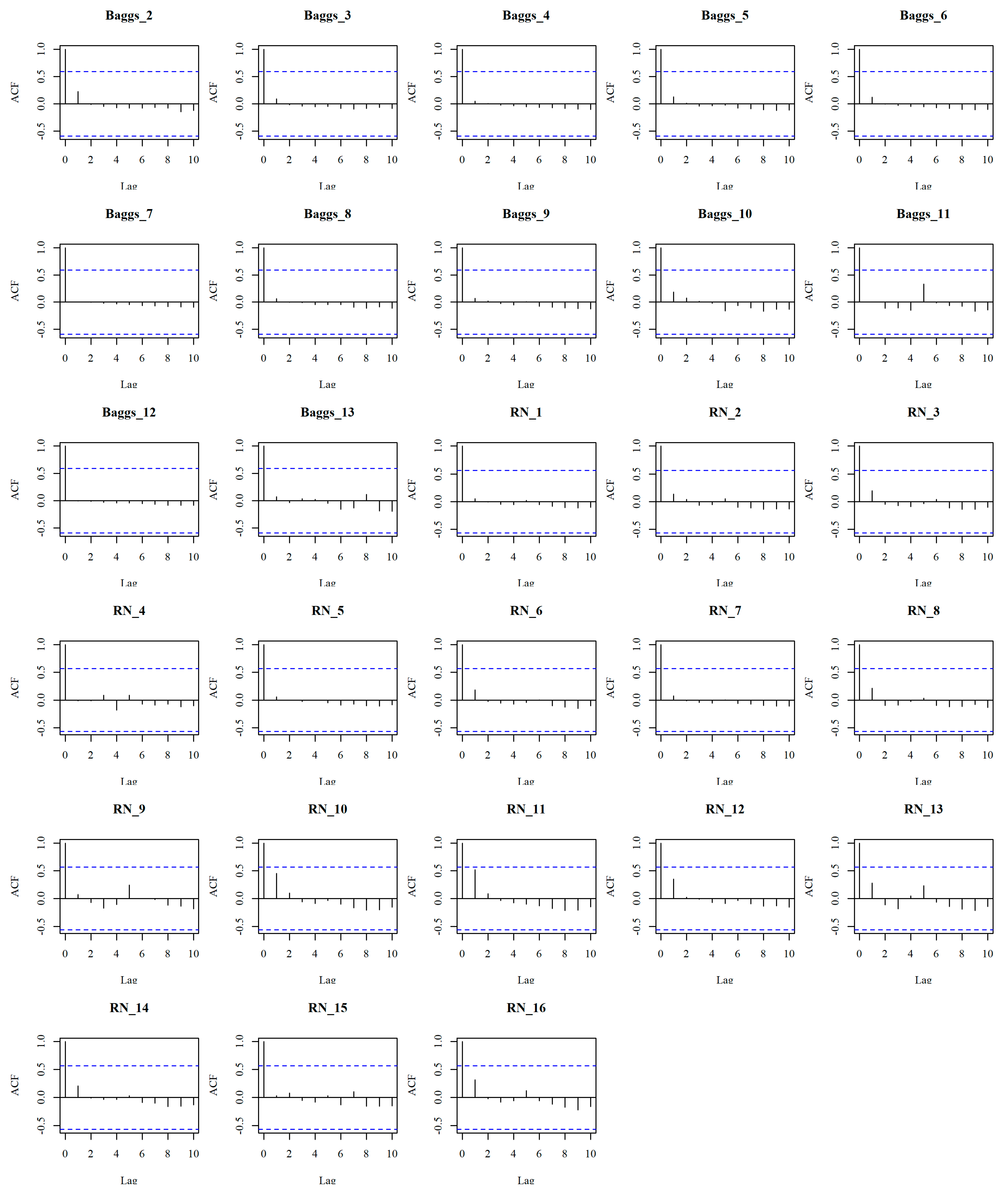
3.1. Testing Autocorrelation
3.2. Training and Testing Data Sampling
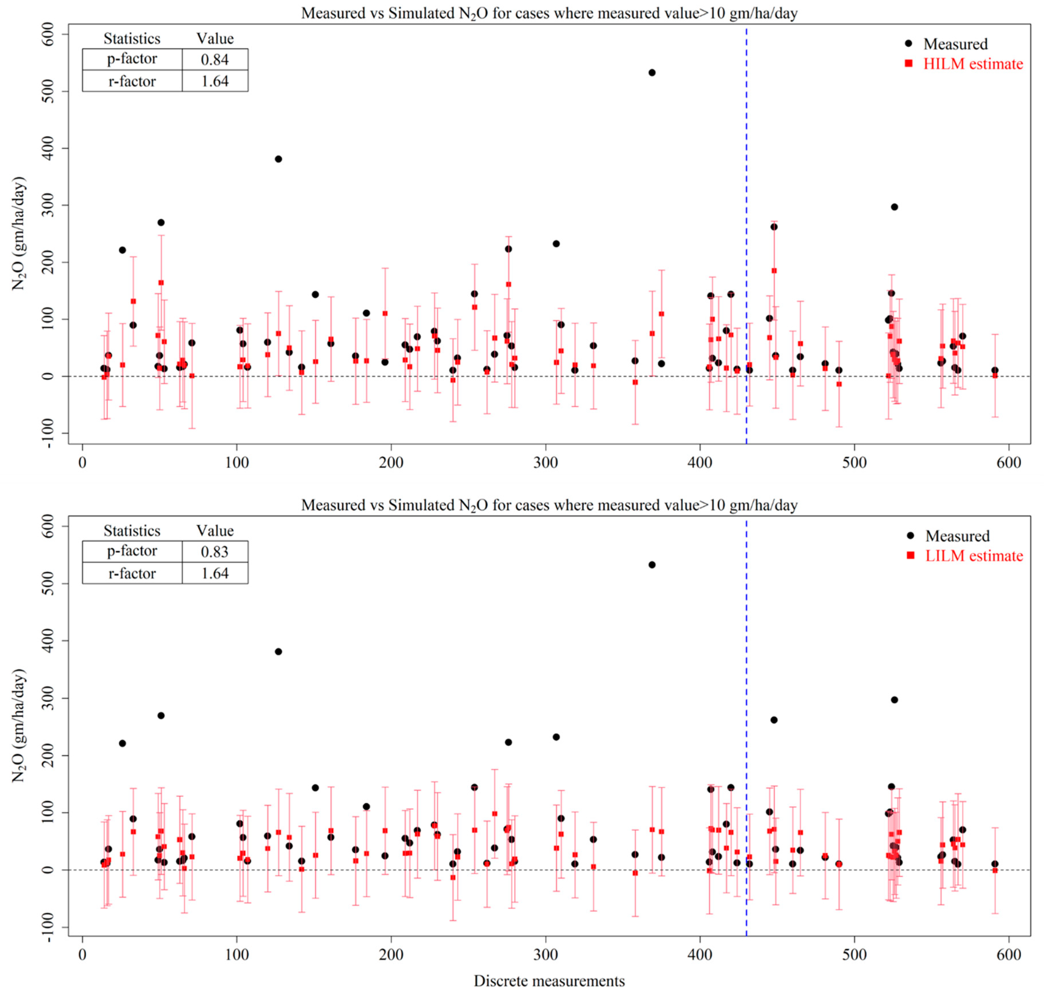
3.3. MLR
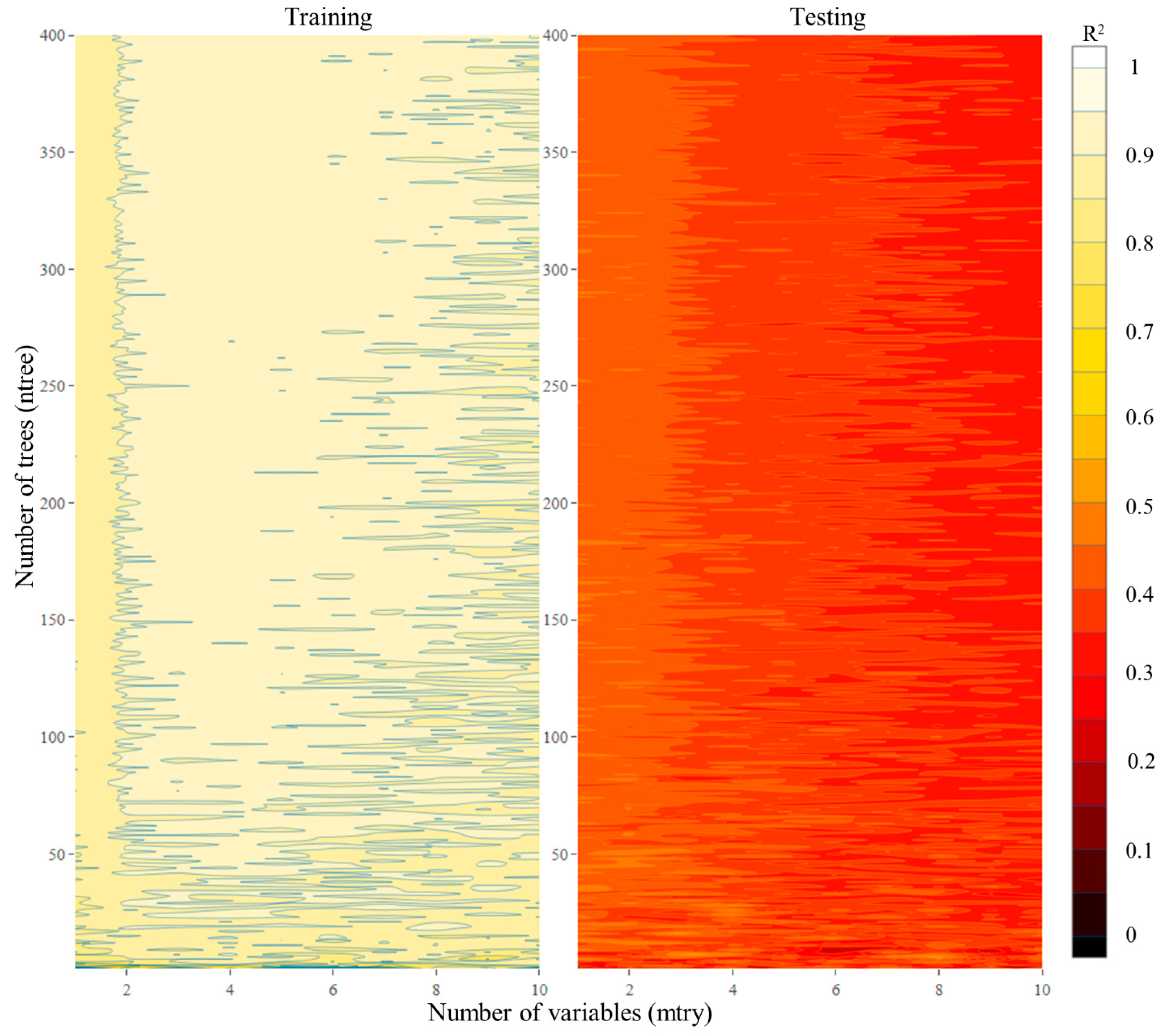
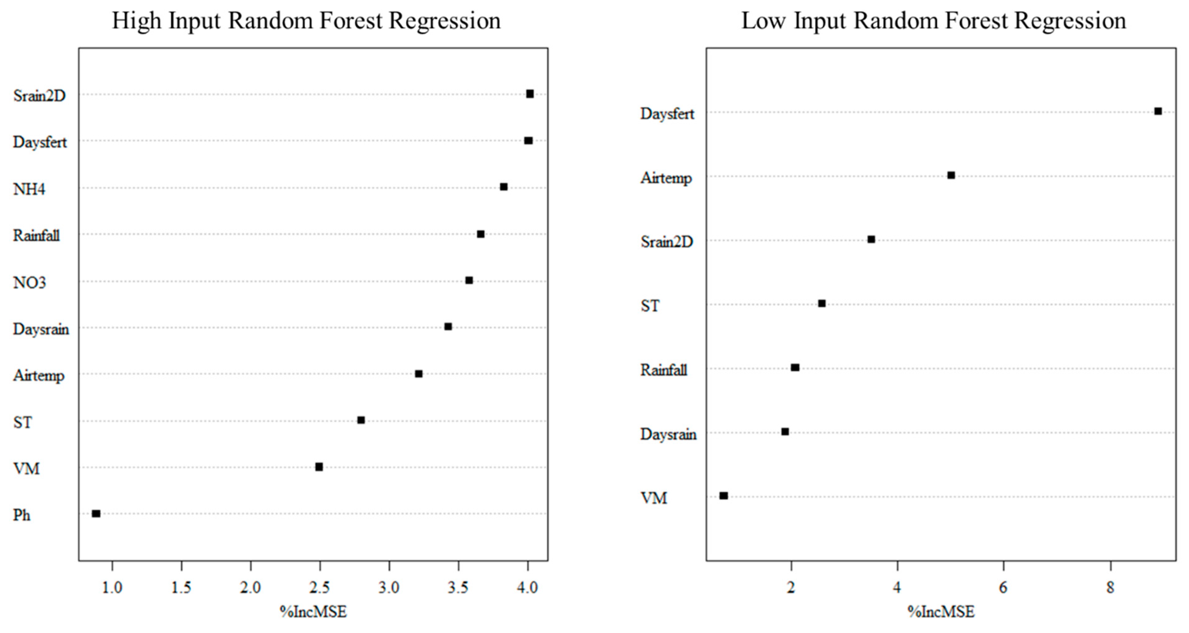
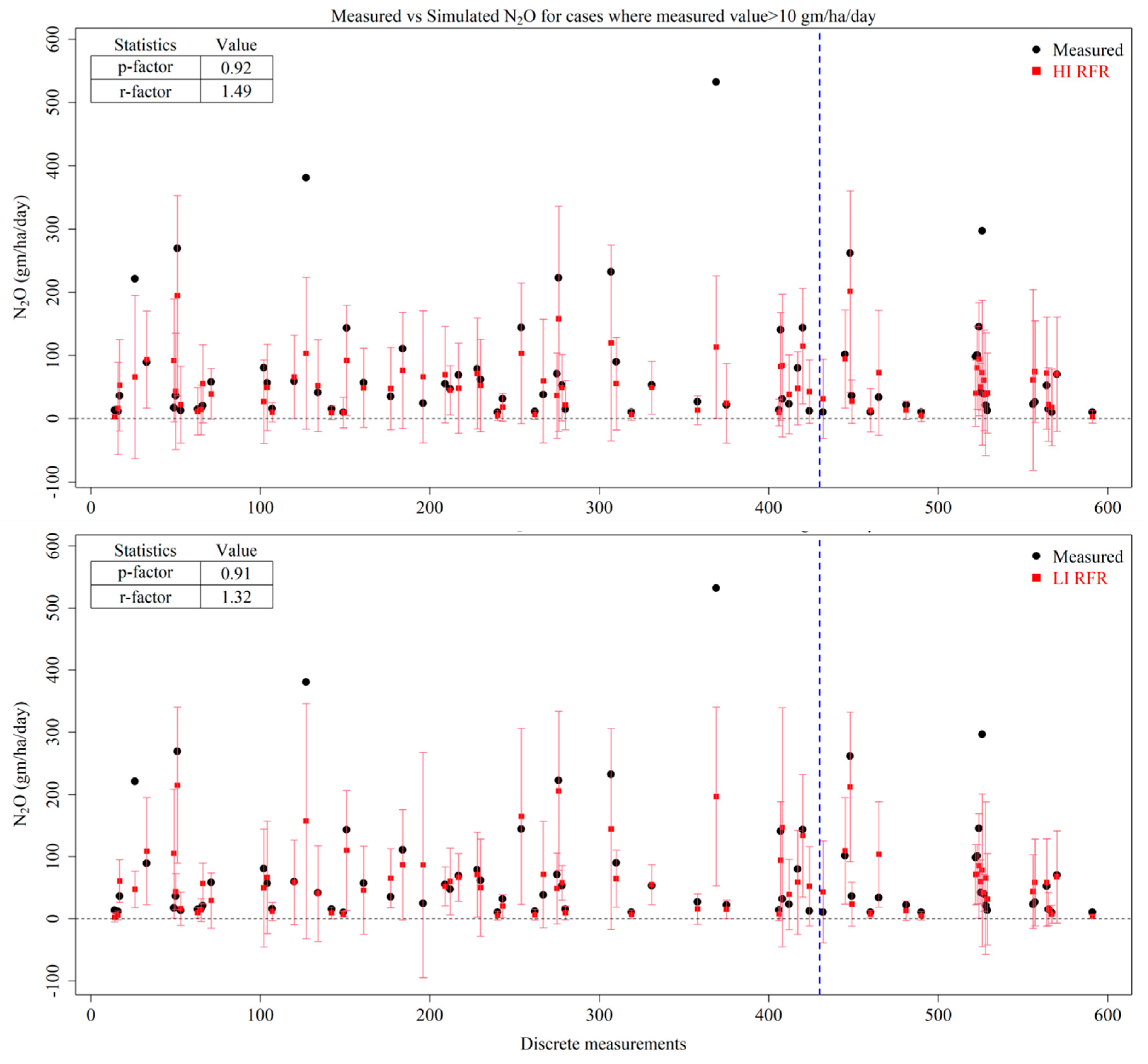
3.4. RFR
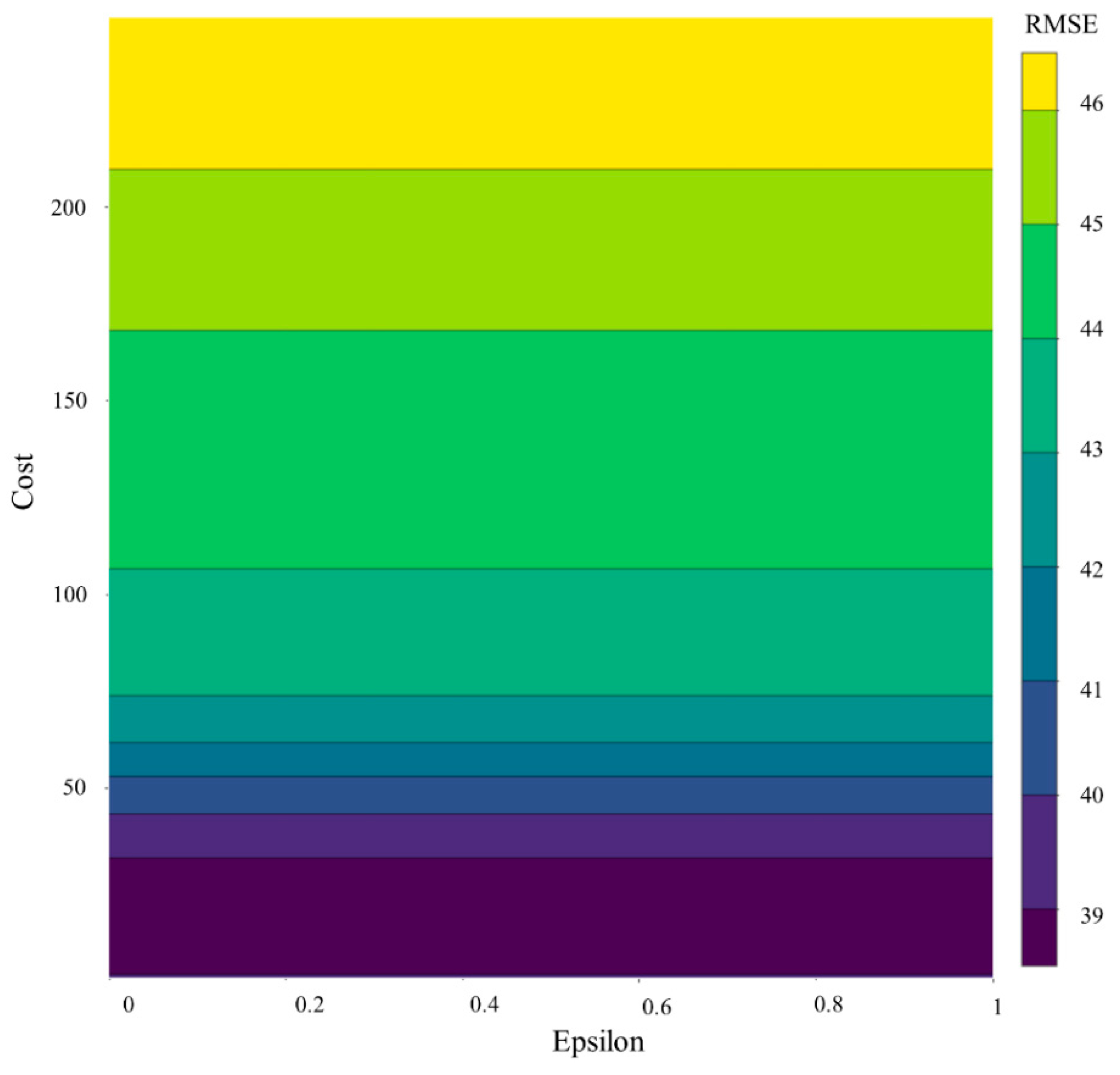
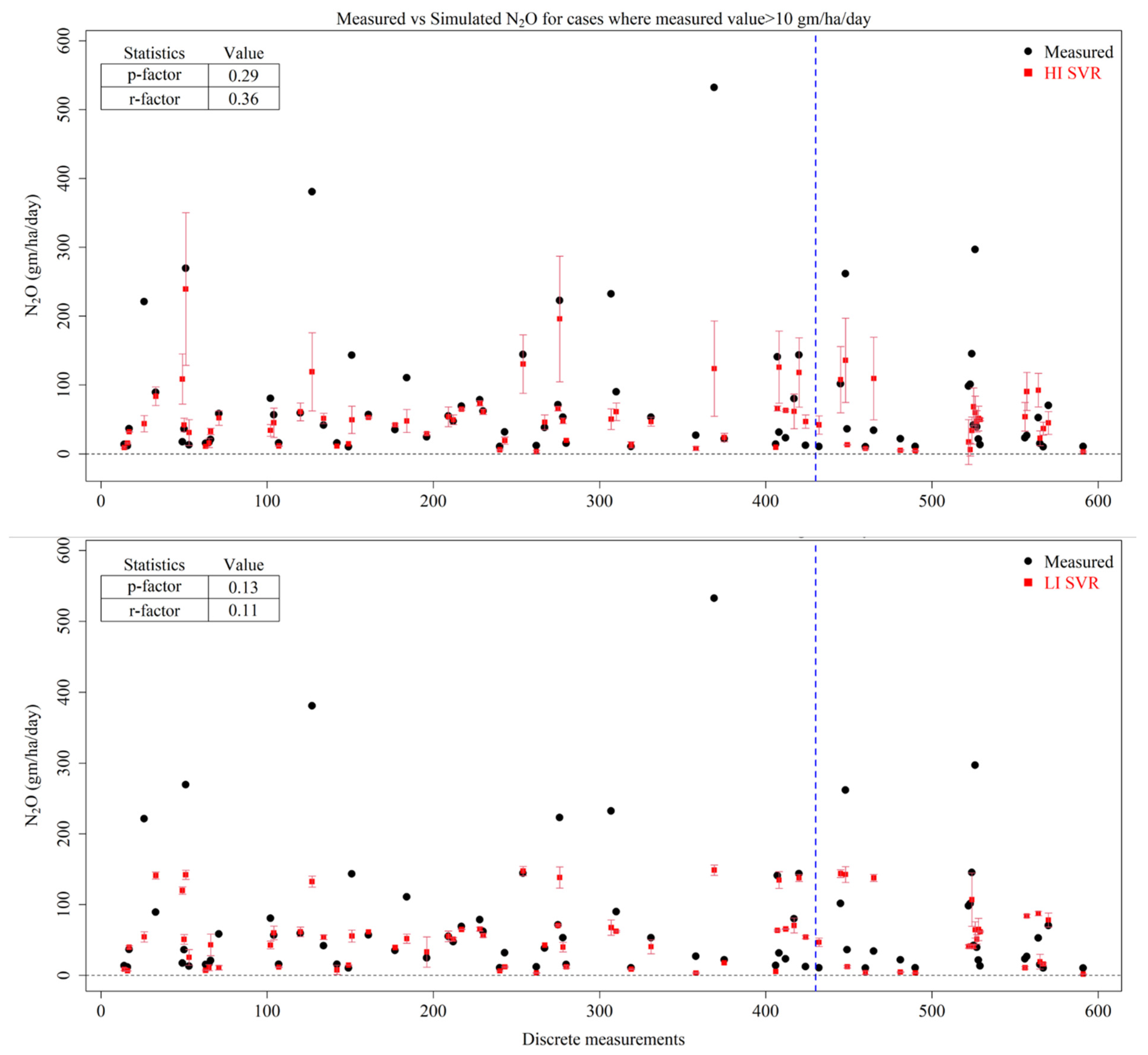
3.5. SVR
3.6. ANN
4. Discussion
5. Conclusions
- There is a need to appropriately split the data into training and testing datasets in such a way that the basic characteristics of the dataset are preserved. There is a considerable band of uncertainty in the results predicted by algorithms trained on different sets of training data.
- The dataset violated the basic assumptions of the MLR application, such as high multicollinearity, heteroscedasticity and no linear relationship between the predictors and predictand N2O variable, thereby rendering the application of MLR invalid. Despite the violation of these assumptions, MLR could not explain more than 30% of the variability of N2O emissions.
- RFR, SVR and ANN could subsequently explain more than 66%, 63% and 43% of the variability of an unseen test dataset when the models were trained for the HI scenario.
- The RFR, SVR and ANN models trained under the LI scenario were found to have comparable performance with models trained under the HI scenario, with subsequent explanations of 68%, 66% and 68% of the variability of the unseen test dataset.
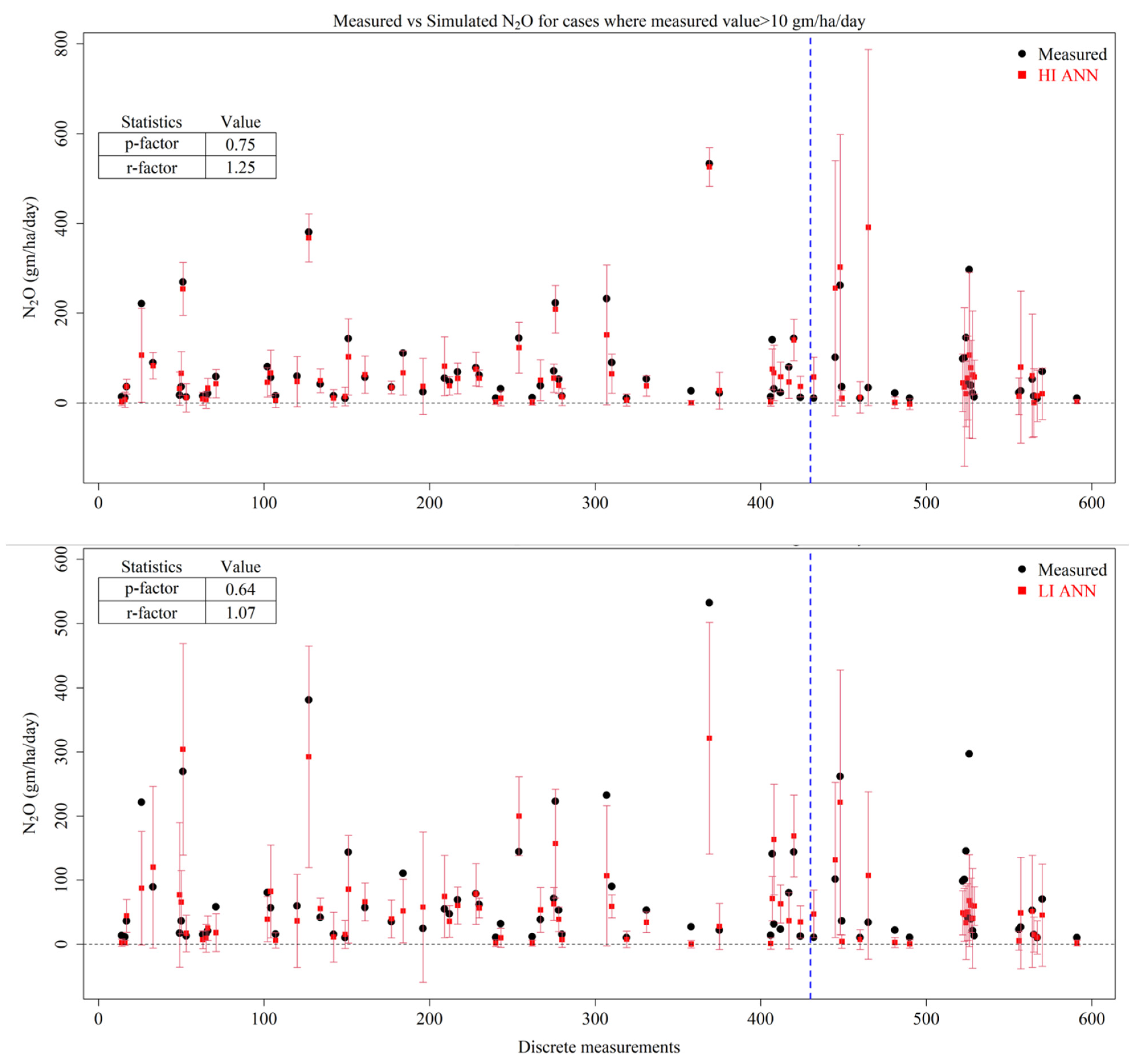
- The peak emissions were better captured by an ANN under the HI scenario, followed by an ANN under the LI scenario, RFR under the HI scenario and RFR under the LI scenario. However, none of the models were able to capture all of the peak emissions within their uncertainty bands.
- Prediction uncertainties were best captured by the RFR and ANN algorithms, with SVM performing very poorly.
- All algorithms were prone to overfitting, thus demanding the careful selection of model parameters and representative training and testing datasets.
- Considering the computational cost, ease in fine-tuning the model, stability of the model results for bootstrapped datasets and a relatively easier interpretation, RFR followed by ANN is recommended for N2O estimation in future studies in the study area.
- There is a merit in using machine learning algorithms trained with local data to estimate N2O emissions in conjunction with readily measurable weather and management variables. However, additional variables known to influence peak emissions need to be included, along with more instances of peak emissions.
- Future studies are recommended to use K-fold cross-validation to generalize the model and avoid biased performance metrices. Similarly, techniques capable of handling epistemic uncertainty in addition to the aleatoric uncertainties stemming from data are recommended.
Supplementary Materials
Author Contributions
Funding
Informed Consent Statement
Data Availability Statement
Conflicts of Interest
References
- Masson-Delmotte, V.; Zhai, P.; Pirani, A.; Connors, S.L.; Péan, C.; Berger, S.; Caud, N.; Chen, Y.; Goldfarb, L.; Gomis, M. Climate change 2021: The physical science basis. In Contribution of Working Group I to the Sixth Assessment Report of the Intergovernmental Panel on Climate Change; IPCC: Geneva, Switzerland, 2021; Volume 2, p. 2391. [Google Scholar]
- Ravishankara, A.; Daniel, J.S.; Portmann, R.W. Nitrous oxide (N2O): The dominant ozone-depleting substance emitted in the 21st century. Science 2009, 326, 123–125. [Google Scholar] [CrossRef] [PubMed]
- Tian, H.; Xu, R.; Canadell, J.G.; Thompson, R.L.; Winiwarter, W.; Suntharalingam, P.; Davidson, E.A.; Ciais, P.; Jackson, R.B.; Janssens-Maenhout, G.; et al. A comprehensive quantification of global nitrous oxide sources and sinks. Nature 2020, 586, 248–256. [Google Scholar] [CrossRef] [PubMed]
- Wohlfahrt, G.; Anfang, C.; Bahn, M.; Haslwanter, A.; Newesely, C.; Schmitt, M.; Drösler, M.; Pfadenhauer, J.; Cernusca, A. Quantifying nighttime ecosystem respiration of a meadow using eddy covariance, chambers and modelling. Agric. For. Meteorol. 2005, 128, 141–162. [Google Scholar] [CrossRef]
- Pavelka, M.; Acosta, M.; Kiese, R.; Altimir, N.; Brümmer, C.; Crill, P.; Darenova, E.; Fuß, R.; Gielen, B.; Graf, A. Standardisation of chamber technique for CO2, N2O and CH4 fluxes measurements from terrestrial ecosystems. Int. Agrophysics 2018, 32, 569–587. [Google Scholar] [CrossRef]
- Denmead, O. Approaches to measuring fluxes of methane and nitrous oxide between landscapes and the atmosphere. Plant Soil 2008, 309, 5–24. [Google Scholar] [CrossRef]
- Korkiakoski, M.; Tuovinen, J.-P.; Aurela, M.; Koskinen, M.; Minkkinen, K.; Ojanen, P.; Penttilä, T.; Rainne, J.; Laurila, T.; Lohila, A. Methane exchange at the peatland forest floor–automatic chamber system exposes the dynamics of small fluxes. Biogeosciences 2017, 14, 1947–1967. [Google Scholar] [CrossRef]
- Nicolini, G.; Castaldi, S.; Fratini, G.; Valentini, R. A literature overview of micrometeorological CH4 and N2O flux measurements in terrestrial ecosystems. Atmos. Environ. 2013, 81, 311–319. [Google Scholar] [CrossRef]
- Giltrap, D.; Yeluripati, J.; Smith, P.; Fitton, N.; Smith, W.; Grant, B.; Dorich, C.D.; Deng, J.; Topp, C.F.; Abdalla, M.; et al. Global Research Alliance N2O chamber methodology guidelines: Summary of modeling approaches. J. Environ. Qual. 2020, 49, 1168–1185. [Google Scholar] [CrossRef]
- Hergoualc’h, K.; Harmand, J.-M.; Cannavo, P.; Skiba, U.; Oliver, R.; Hénault, C. The utility of process-based models for simulating N2O emissions from soils: A case study based on Costa Rican coffee plantations. Soil Biol. Biochem. 2009, 41, 2343–2355. [Google Scholar] [CrossRef]
- Leip, A.; Busto, M.; Corazza, M.; Bergamaschi, P.; Koeble, R.; Dechow, R.; Monni, S.; De Vries, W. Estimation of N2O fluxes at the regional scale: Data, models, challenges. Curr. Opin. Environ. Sustain. 2011, 3, 328–338. [Google Scholar] [CrossRef]
- Fuchs, K.; Merbold, L.; Buchmann, N.; Bellocchi, G.; Bindi, M.; Brilli, L.; Conant, R.T.; Dorich, C.D.; Ehrhardt, F.; Fitton, N.; et al. Evaluating the potential of legumes to mitigate N2O emissions from permanent grassland using process-based models. Glob. Biogeochem. Cycles 2020, 34, e2020GB006561. [Google Scholar] [CrossRef]
- Vogeler, I.; Cichota, R. Effect of variability in soil properties plus model complexity on predicting topsoil water content and nitrous oxide emissions. Soil Res. 2018, 56, 810–819. [Google Scholar] [CrossRef]
- Gaillard, R.K.; Jones, C.D.; Ingraham, P.; Collier, S.; Izaurralde, R.C.; Jokela, W.; Osterholz, W.; Salas, W.; Vadas, P.; Ruark, M.D. Underestimation of N2O emissions in a comparison of the DayCent, DNDC, and EPIC models. Ecol. Appl. 2018, 28, 694–708. [Google Scholar] [CrossRef]
- Yue, Q.; Cheng, K.; Ogle, S.; Hillier, J.; Smith, P.; Abdalla, M.; Ledo, A.; Sun, J.; Pan, G. Evaluation of four modelling approaches to estimate nitrous oxide emissions in China’s cropland. Sci. Total Environ. 2019, 652, 1279–1289. [Google Scholar] [CrossRef]
- Ghimire, U.; Shrestha, N.K.; Biswas, A.; Wagner-Riddle, C.; Yang, W.; Prasher, S.; Rudra, R.; Daggupati, P. A Review of Ongoing Advancements in Soil and Water Assessment Tool (SWAT) for Nitrous Oxide (N2O) Modeling. Atmosphere 2020, 11, 450. [Google Scholar] [CrossRef]
- Wang, C.; Amon, B.; Schulz, K.; Mehdi, B. Factors that influence nitrous oxide emissions from agricultural soils as well as their representation in simulation models: A review. Agronomy 2021, 11, 770. [Google Scholar] [CrossRef]
- Fisher, R.A.; Koven, C.D. Perspectives on the future of land surface models and the challenges of representing complex terrestrial systems. J. Adv. Model. Earth Syst. 2020, 12, e2018MS001453. [Google Scholar] [CrossRef]
- Berardi, D.; Brzostek, E.; Blanc-Betes, E.; Davison, B.; DeLucia, E.H.; Hartman, M.D.; Kent, J.; Parton, W.J.; Saha, D.; Hudiburg, T.W. 21st-century biogeochemical modeling: Challenges for Century-based models and where do we go from here? GCB Bioenergy 2020, 12, 774–788. [Google Scholar] [CrossRef]
- Vasilaki, V.; Massara, T.; Stanchev, P.; Fatone, F.; Katsou, E. A decade of nitrous oxide (N2O) monitoring in full-scale wastewater treatment processes: A critical review. Water Res. 2019, 161, 392–412. [Google Scholar] [CrossRef]
- Gao, X.; Ouyang, W.; Hao, Z.; Xie, X.; Lian, Z.; Hao, X.; Wang, X. SWAT-N2O coupler: An integration tool for soil N2O emission modeling. Environ. Model. Softw. 2019, 115, 86–97. [Google Scholar] [CrossRef]
- Wagena, M.B.; Bock, E.M.; Sommerlot, A.R.; Fuka, D.R.; Easton, Z.M. Development of a nitrous oxide routine for the SWAT model to assess greenhouse gas emissions from agroecosystems. Environ. Model. Softw. 2017, 89, 131–143. [Google Scholar] [CrossRef]
- Mehrani, M.-J.; Bagherzadeh, F.; Zheng, M.; Kowal, P.; Sobotka, D.; Mąkinia, J. Application of a hybrid mechanistic/machine learning model for prediction of nitrous oxide (N2O) production in a nitrifying sequencing batch reactor. Process Saf. Environ. Prot. 2022, 162, 1015–1024. [Google Scholar] [CrossRef]
- Wang, C.; Schürz, C.; Zoboli, O.; Zessner, M.; Schulz, K.; Watzinger, A.; Bodner, G.; Mehdi-Schulz, B. N2O Emissions from Two Austrian Agricultural Catchments Simulated with an N2O Submodule Developed for the SWAT Model. Atmosphere 2021, 13, 50. [Google Scholar] [CrossRef]
- Shrestha, N.K.; Thomas, B.W.; Du, X.; Hao, X.; Wang, J. Modeling nitrous oxide emissions from rough fescue grassland soils subjected to long-term grazing of different intensities using the Soil and Water Assessment Tool (SWAT). Environ. Sci. Pollut. Res. 2018, 25, 27362–27377. [Google Scholar] [CrossRef]
- Saha, D.; Basso, B.; Robertson, G.P. Machine learning improves predictions of agricultural nitrous oxide (N2O) emissions from intensively managed cropping systems. Environ. Res. Lett. 2021, 16, 024004. [Google Scholar] [CrossRef]
- Chen, Z.; Ding, W.; Luo, Y.; Yu, H.; Xu, Y.; Müller, C.; Xu, X.; Zhu, T. Nitrous oxide emissions from cultivated black soil: A case study in Northeast China and global estimates using empirical model. Glob. Biogeochem. Cycles 2014, 28, 1311–1326. [Google Scholar] [CrossRef]
- Song, K.; Park, Y.-S.; Zheng, F.; Kang, H. The application of Artificial Neural Network (ANN) model to the simulation of denitrification rates in mesocosm-scale wetlands. Ecol. Inform. 2013, 16, 10–16. [Google Scholar] [CrossRef]
- Philibert, A.; Loyce, C.; Makowski, D. Prediction of N2O emission from local information with Random Forest. Environ. Pollut. 2013, 177, 156–163. [Google Scholar] [CrossRef] [PubMed]
- Saha, D.; Kemanian, A.R.; Rau, B.M.; Adler, P.R.; Montes, F. Designing efficient nitrous oxide sampling strategies in agroecosystems using simulation models. Atmos. Environ. 2017, 155, 189–198. [Google Scholar] [CrossRef]
- Taki, R.; Wagner-Riddle, C.; Parkin, G.; Gordon, R.; VanderZaag, A. Comparison of two gap-filling techniques for nitrous oxide fluxes from agricultural soil. Can. J. Soil Sci. 2018, 99, 12–24. [Google Scholar] [CrossRef]
- Bigaignon, L.; Fieuzal, R.; Delon, C.; Tallec, T. Combination of two methodologies, artificial neural network and linear interpolation, to gap-fill daily nitrous oxide flux measurements. Agric. For. Meteorol. 2020, 291, 108037. [Google Scholar] [CrossRef]
- Goodrich, J.; Wall, A.; Campbell, D.; Fletcher, D.; Wecking, A.; Schipper, L.J.A.; Meteorology, F. Improved gap filling approach and uncertainty estimation for eddy covariance N2O fluxes. Agric. For. Meteorol. 2021, 297, 108280. [Google Scholar] [CrossRef]
- Stehfest, E.; Bouwman, L. N2O and NO emission from agricultural fields and soils under natural vegetation: Summarizing available measurement data and modeling of global annual emissions. Nutr. Cycl. Agroecosystems 2006, 74, 207–228. [Google Scholar] [CrossRef]
- Maier, R.; Hörtnagl, L.; Buchmann, N. Greenhouse gas fluxes (CO2, N2O and CH4) of pea and maize during two cropping seasons: Drivers, budgets, and emission factors for nitrous oxide. Sci. Total Environ. 2022, 849, 157541. [Google Scholar] [CrossRef]
- Mehmandoost Kotlar, A.; Singh, J.; Kumar, S. Prediction of greenhouse gas emissions from agricultural fields with and without cover crops. Soil Sci. Soc. Am. J. 2022, 86, 1227–1240. [Google Scholar] [CrossRef]
- Wang, Y.; Basu, S. Using an artificial neural network approach to estimate surface-layer optical turbulence at Mauna Loa, Hawaii. Opt. Lett. 2016, 41, 2334–2337. [Google Scholar] [CrossRef]
- Shikhovtsev, A.Y.; Kovadlo, P.G.; Kiselev, A.V.; Eselevich, M.V.; Lukin, V.P. Application of Neural Networks to Estimation and Prediction of Seeing at the Large Solar Telescope Site. Publ. Astron. Soc. Pac. 2023, 135, 014503. [Google Scholar] [CrossRef]
- Carranza, C.; Nolet, C.; Pezij, M.; van der Ploeg, M. Root zone soil moisture estimation with Random Forest. J. Hydrol. 2021, 593, 125840. [Google Scholar] [CrossRef]
- Zhao, W.; Sánchez, N.; Lu, H.; Li, A. A spatial downscaling approach for the SMAP passive surface soil moisture product using random forest regression. J. Hydrol. 2018, 563, 1009–1024. [Google Scholar] [CrossRef]
- Feng, Y.; Cui, N.; Hao, W.; Gao, L.; Gong, D. Estimation of soil temperature from meteorological data using different machine learning models. Geoderma 2019, 338, 67–77. [Google Scholar] [CrossRef]
- Nemitz, E.; Mammarella, I.; Ibrom, A.; Aurela, M.; Burba, G.G.; Dengel, S.; Gielen, B.; Grelle, A.; Heinesch, B.; Herbst, M.; et al. Standardisation of eddy-covariance flux measurements of methane and nitrous oxide. Int. Agrophysics 2018, 32, 517–549. [Google Scholar] [CrossRef]
- Dorich, C.D.; De Rosa, D.; Barton, L.; Grace, P.; Rowlings, D.; Migliorati, M.D.A.; Wagner-Riddle, C.; Key, C.; Wang, D.; Fehr, B.; et al. Global Research Alliance N2O chamber methodology guidelines: Guidelines for gap-filling missing measurements. J. Environ. Qual. 2020, 49, 1186–1202. [Google Scholar] [CrossRef]
- Ashiq, W.; Ghimire, U.; Vasava, H.; Dunfield, K.; Wagner-Riddle, C.; Daggupati, P.; Biswas, A. Identifying hotspots and representative monitoring locations of field scale N2O emissions from agricultural soils: A time stability analysis. Sci. Total Environ. 2021, 788, 147955. [Google Scholar] [CrossRef] [PubMed]
- Ashiq, W.; Vasava, H.; Ghimire, U.; Dunfield, K.; Daggupati, P.; Biswas, A. Seasonal agricultural wetlands act as potential source of N2O and CH4 emissions. CATENA 2022, 213, 106184. [Google Scholar] [CrossRef]
- Pinheiro, J. Nlme: Linear and Nonlinear Mixed Effects Models, Version 3.1-164. 2011. Available online: https://cran.r-project.org/web/packages/nlme/index.html (accessed on 25 February 2024).
- Entekhabi, D.; Njoku, E.G.; O’Neill, P.E.; Kellogg, K.H.; Crow, W.T.; Edelstein, W.N.; Entin, J.K.; Goodman, S.D.; Jackson, T.J.; Johnson, J.; et al. The soil moisture active passive (SMAP) mission. Proc. IEEE 2010, 98, 704–716. [Google Scholar] [CrossRef]
- Wulder, M.A.; Loveland, T.R.; Roy, D.P.; Crawford, C.J.; Masek, J.G.; Woodcock, C.E.; Allen, R.G.; Anderson, M.C.; Belward, A.S.; Cohen, W.B.; et al. Current status of Landsat program, science, and applications. Remote Sens. Environ. 2019, 225, 127–147. [Google Scholar] [CrossRef]
- Pedhazur, E.J.; Schmelkin, L.P. Measurement, Design, and Analysis: An Integrated Approach; Psychology Press: London, UK, 2013. [Google Scholar]
- Tabachnick, B.G.; Fidell, L.S.; Ullman, J.B. Using Multivariate Statistics; Pearson: Boston, MA, USA, 2007; Volume 5. [Google Scholar]
- Bujang, M.A.; Sa’at, N.; Bakar, T.M.I.T.A. Determination of minimum sample size requirement for multiple linear regression and analysis of covariance based on experimental and non-experimental studies. Epidemiol. Biostat. Public Health 2017, 14. [Google Scholar] [CrossRef]
- Zhuang, Q.; Lu, Y.; Chen, M. An inventory of global N2O emissions from the soils of natural terrestrial ecosystems. Atmos. Environ. 2012, 47, 66–75. [Google Scholar] [CrossRef]
- Abbasi, T.; Luithui, C.; Abbasi, S.A. Modelling methane and nitrous oxide emissions from rice paddy wetlands in India using artificial neural networks (ANNs). Water 2019, 11, 2169. [Google Scholar] [CrossRef]
- Korkiakoski, M.; Ojanen, P.; Penttilä, T.; Minkkinen, K.; Sarkkola, S.; Rainne, J.; Laurila, T.; Lohila, A. Impact of partial harvest on CH4 and N2O balances of a drained boreal peatland forest. Agric. For. Meteorol. 2020, 295, 108168. [Google Scholar] [CrossRef]
- Uyanık, G.K.; Güler, N. A study on multiple linear regression analysis. Procedia-Soc. Behav. Sci. 2013, 106, 234–240. [Google Scholar] [CrossRef]
- Grégoire, G. Multiple linear regression. Eur. Astron. Soc. Publ. Ser. 2014, 66, 45–72. [Google Scholar] [CrossRef]
- Fox, J.; Weisberg, S.; Adler, D.; Bates, D.; Baud-Bovy, G.; Ellison, S.; Firth, D.; Friendly, M.; Gorjanc, G.; Graves, S. Package ‘car’. R Foundation for Statistical Computing. 2012. Available online: https://cran.r-project.org/web/packages/car/index.html (accessed on 25 February 2024).
- James, G.; Witten, D.; Hastie, T.; Tibshirani, R. An Introduction to Statistical Learning; Springer: Berlin/Heidelberg, Germany, 2013; Volume 112. [Google Scholar]
- Breiman, L.; Cutler, A. randomForest: Breiman and Cutler’s random forests for classification and regression. CRAN Contrib. Packages 2018, 4, 6–14. [Google Scholar]
- Vapnik, V.N. An overview of statistical learning theory. IEEE Trans. Neural Netw. 1999, 10, 988–999. [Google Scholar] [CrossRef] [PubMed]
- Géron, A. Hands-on Machine Learning with Scikit-Learn, Keras, and TensorFlow; O’Reilly Media, Inc.: Sebastopol, CA, USA, 2022. [Google Scholar]
- Seok, K.; Hwang, C.; Cho, D. Prediction intervals for support vector machine regression. Commun. Stat.-Theory Methods 2002, 31, 1887–1898. [Google Scholar] [CrossRef]
- Steinwart, I.; Christmann, A. Support Vector Machines; Springer Science & Business Media: Berlin/Heidelberg, Germany, 2008. [Google Scholar]
- Meyer, D.; Dimitriadou, E.; Hornik, K.; Weingessel, A.; Leisch, F.; Chang, C.-C.; Lin, C.-C.; Meyer, M.D. Package ‘e1071’. 2019. Available online: https://cran.r-project.org/web/packages/e1071/index.html (accessed on 25 February 2024).
- Awad, M.; Khanna, R. Support vector regression. In Efficient Learning Machines; Springer: Berlin/Heidelberg, Germany, 2015; pp. 67–80. [Google Scholar]
- Shaahmadi, F.; Anbaz, M.A.; Bazooyar, B. Analysis of intelligent models in prediction nitrous oxide (N2O) solubility in ionic liquids (ILs). J. Mol. Liq. 2017, 246, 48–57. [Google Scholar] [CrossRef]
- Kazemi, P.; Bengoa, C.; Steyer, J.-P.; Giralt, J. Data-driven techniques for fault detection in anaerobic digestion process. Process Saf. Environ. Prot. 2021, 146, 905–915. [Google Scholar] [CrossRef]
- Fritsch, S.; Guenther, F.; Guenther, M.F. Package ‘neuralnet’. The Comprehensive R Archive Network. 2016. Available online: https://cran.r-project.org/web/packages/neuralnet/neuralnet.pdf (accessed on 15 March 2024).
- Lin, C. Analysis of Complex Dynamical Systems by Combining Recurrent Neural Networks and Mechanistic Models. Ph.D. Thesis, University of Ottawa, Ottawa, ON, Canada, 2024. [Google Scholar]
- Nourani, V.; Paknezhad, N.J.; Tanaka, H. Prediction Interval Estimation Methods for Artificial Neural Network (ANN)-based modeling of the hydro-climatic processes, a review. Sustainability 2021, 13, 1633. [Google Scholar] [CrossRef]
- Lu, B.; Hardin, J. Constructing Prediction Intervals for Random Forests. Ph.D. Thesis, Pomona College, Claremont, CA, USA, 2017. [Google Scholar]
- Coulston, J.W.; Blinn, C.E.; Thomas, V.A.; Wynne, R.H. Approximating prediction uncertainty for random forest regression models. Photogramm. Eng. Remote Sens. 2016, 82, 189–197. [Google Scholar] [CrossRef]
- Lins, I.D.; Droguett, E.L.; das Chagas Moura, M.; Zio, E.; Jacinto, C.M. Computing confidence and prediction intervals of industrial equipment degradation by bootstrapped support vector regression. Reliab. Eng. Syst. Saf. 2015, 137, 120–128. [Google Scholar] [CrossRef]
- Xu, Y.; Mi, C.; Zhu, Q.-X.; Gao, J.-Y.; He, Y.-L. An effective high-quality prediction intervals construction method based on parallel bootstrapped RVM for complex chemical processes. Chemom. Intell. Lab. Syst. 2017, 171, 161–169. [Google Scholar] [CrossRef]
- Lian, C.; Chen, C.P.; Zeng, Z.; Yao, W.; Tang, H. Prediction intervals for landslide displacement based on switched neural networks. IEEE Trans. Reliab. 2016, 65, 1483–1495. [Google Scholar] [CrossRef]
- Kasiviswanathan, K.; Cibin, R.; Sudheer, K.; Chaubey, I. Constructing prediction interval for artificial neural network rainfall runoff models based on ensemble simulations. J. Hydrol. 2013, 499, 275–288. [Google Scholar] [CrossRef]
- Abbaspour, K.C.; Yang, J.; Maximov, I.; Siber, R.; Bogner, K.; Mieleitner, J.; Zobrist, J.; Srinivasan, R. Modelling hydrology and water quality in the pre-alpine/alpine Thur watershed using SWAT. J. Hydrol. 2007, 333, 413–430. [Google Scholar] [CrossRef]
- Esmali, A.; Golshan, M.; Kavian, A. Investigating the performance of SWAT and IHACRES in simulation streamflow under different climatic regions in Iran. Atmósfera 2021, 34, 79–96. [Google Scholar] [CrossRef]
- Zambrano-Bigiarini, M. “Package ‘hydroGOF’.” Goodness-of-fit Functions for Comparison of Simulated and Observed (2017). 2017. Available online: https://cran.r-project.org/web/packages/hydroGOF/index.html (accessed on 7 January 2024).
- Batra, R.; Johal, S.K.; Chen, M.; Ferrer, E. Consequences of sampling frequency on the estimated dynamics of AR processes using continuous-time models. Psychol. Methods 2023. [Google Scholar] [CrossRef]
- Chirinda, N.; Carter, M.S.; Albert, K.R.; Ambus, P.; Olesen, J.E.; Porter, J.R.; Petersen, S.O. Emissions of nitrous oxide from arable organic and conventional cropping systems on two soil types. Agric. Ecosyst. Environ. 2010, 136, 199–208. [Google Scholar] [CrossRef]
- Butterbach-Bahl, K.; Baggs, E.M.; Dannenmann, M.; Kiese, R.; Zechmeister-Boltenstern, S. Nitrous oxide emissions from soils: How well do we understand the processes and their controls? Philos. Trans. R. Soc. B Biol. Sci. 2013, 368, 20130122. [Google Scholar] [CrossRef]
- Ciarlo, E.; Conti, M.; Bartoloni, N.; Rubio, G. The effect of moisture on nitrous oxide emissions from soil and the N2O/(N2O+ N2) ratio under laboratory conditions. Biol. Fertil. Soils 2007, 43, 675–681. [Google Scholar] [CrossRef]
- Clayton, H.; McTaggart, I.; Parker, J.; Swan, L.; Smith, K. Nitrous oxide emissions from fertilised grassland: A 2-year study of the effects of N fertiliser form and environmental conditions. Biol. Fertil. Soils 1997, 25, 252–260. [Google Scholar] [CrossRef]
- Van Haren, J.L.; de Oliveira, R.C., Jr.; Restrepo-Coupe, N.; Hutyra, L.; De Camargo, P.B.; Keller, M.; Saleska, S.R. Do plant species influence soil CO2 and N2O fluxes in a diverse tropical forest? J. Geophys. Res. Biogeosci. 2010, 115. [Google Scholar] [CrossRef]
- Li, Y.; Barton, L.; Chen, D. Simulating response of N2O emissions to fertiliser N application and climatic variability from a rain-fed and wheat-cropped soil in Western Australia. J. Sci. Food Agric. 2012, 92, 1130–1143. [Google Scholar] [CrossRef] [PubMed]
- Nishina, K.; Akiyama, H.; Nishimura, S.; Sudo, S.; Yagi, K. Evaluation of uncertainties in N2O and NO fluxes from agricultural soil using a hierarchical Bayesian model. J. Geophys. Res. Biogeosci. 2012, 117. [Google Scholar] [CrossRef]
- Lugato, E.; Paniagua, L.; Jones, A.; de Vries, W.; Leip, A. Complementing the topsoil information of the Land Use/Land Cover Area Frame Survey (LUCAS) with modelled N2O emissions. PLoS ONE 2017, 12, e0176111. [Google Scholar] [CrossRef]
- Villa-Vialaneix, N.; Follador, M.; Ratto, M.; Leip, A. A comparison of eight metamodeling techniques for the simulation of N2O fluxes and N leaching from corn crops. Environ. Model. Softw. 2012, 34, 51–66. [Google Scholar] [CrossRef]
- Liu, Q.; Liu, B.; Zhang, Y.; Hu, T.; Lin, Z.; Liu, G.; Wang, X.; Ma, J.; Wang, H.; Jin, H.; et al. Biochar application as a tool to decrease soil nitrogen losses (NH3 volatilization, N2O emissions, and N leaching) from croplands: Options and mitigation strength in a global perspective. Glob. Change Biol. 2019, 25, 2077–2093. [Google Scholar] [CrossRef]
- Were, K.; Bui, D.T.; Dick, Ø.B.; Singh, B.R. A comparative assessment of support vector regression, artificial neural networks, and random forests for predicting and mapping soil organic carbon stocks across an Afromontane landscape. Ecol. Indic. 2015, 52, 394–403. [Google Scholar] [CrossRef]
- Kohli, S.; Miglani, S.; Rapariya, R. Basics of artificial neural network. Int. J. Comput. Sci. Mob. Comput. 2014, 3, 745–751. [Google Scholar]
- Ghazali, M.F.; Wikantika, K.; Harto, A.B.; Kondoh, A. Generating soil salinity, soil moisture, soil pH from satellite imagery and its analysis. Inf. Process. Agric. 2020, 7, 294–306. [Google Scholar] [CrossRef]
- Li, B.; Ti, C.; Zhao, Y.; Yan, X. Estimating soil moisture with Landsat data and its application in extracting the spatial distribution of winter flooded paddies. Remote Sens. 2016, 8, 38. [Google Scholar] [CrossRef]
- Mobasheri, M.R.; Amani, M. Soil moisture content assessment based on Landsat 8 red, near-infrared, and thermal channels. J. Appl. Remote Sens. 2016, 10, 026011. [Google Scholar] [CrossRef]
- Du, C.; Ren, H.; Qin, Q.; Meng, J.; Zhao, S. A practical split-window algorithm for estimating land surface temperature from Landsat 8 data. Remote Sens. 2015, 7, 647–665. [Google Scholar] [CrossRef]
- Meng, X.; Cheng, J.; Zhao, S.; Liu, S.; Yao, Y. Estimating land surface temperature from Landsat-8 data using the NOAA JPSS enterprise algorithm. Remote Sens. 2019, 11, 155. [Google Scholar] [CrossRef]
- Myrgiotis, V.; Williams, M.; Topp, C.F.; Rees, R.M. Improving model prediction of soil N2O emissions through Bayesian calibration. Sci. Total Environ. 2018, 624, 1467–1477. [Google Scholar] [CrossRef]
- Hashimoto, S.; Morishita, T.; Sakata, T.; Ishizuka, S.; Kaneko, S.; Takahashi, M. Simple models for soil CO2, CH4, and N2O fluxes calibrated using a Bayesian approach and multi-site data. Ecol. Model. 2011, 222, 1283–1292. [Google Scholar] [CrossRef]


| Variable | Description | Units | Range in the Available Data (Min, Max) |
|---|---|---|---|
| ST | Soil temperature at 10–15 cm depth | °C | 0.12, 27.75 |
| VM | Soil volumetric moisture at 10–15 cm depth | % | 5.1, 58.3 |
| pH | pH value of the soil | - | 6.08, 7.89 |
| Daysrain | Number of days after last rainfall | - | 0, 7 |
| Rainfall | Cumulative rainfall on the day of N2O measurement | mm | 0, 10.9 |
| Airtemp | Average air temperature on the day of N2O measurement | °C | −1.8, 24.9 |
| Daysfert | Number of days after application of nitrogenous fertilizer (inorganic) | - | 7, 489 |
| NH4 | Soil ammonium content at 10–15 cm depth | mg/kg | 0, 89.32 |
| NO3 | Soil nitrate concentration at 10–15 cm depth | mg/kg | 0, 110.40 |
| Srain2D | Accumulated 2-day rainfall on the day of N2O measurement | mm | 0, 37.7 |
| N2O | Average N2O flux in the given day | gm N2O-N/ha/day | −26.88, 532.34 |
| Variable | VIF-HILMo | VIF-HILM | VIF-LILMo | VIF-LILM |
|---|---|---|---|---|
| ST | 7.644 | 14,585 | 7.028 | 29.359 |
| VM | 2.732 | 10,799 | 2.578 | 17.846 |
| Ph | 1.236 | 98.59 | ||
| Daysrain | 1.79 | 2.19 | 1.784 | 51.775 |
| Rainfall | 1.422 | 1.64 | 1.414 | 1.441 |
| Airtemp | 5.236 | 6.07 | 5.099 | 5.816 |
| Daysfert | 1.721 | 1.94 | 1.153 | 1.215 |
| NH4 | 1.066 | 1.29 | ||
| NO3 | 1.65 | 166,292 | ||
| Srain2D | 1.65 | 1.84 | 1.603 | 1.832 |
| ST: VM | 8233 | 10.519 | ||
| ST: Daysrain | 35.761 | |||
| ST: Ph | 14,886 | |||
| VM: Ph | 10,517 | |||
| VM: Daysrain | 39.08 | |||
| ST: NO3 | 166,779 | |||
| VM: NO3 | 133,735 | |||
| Ph: NO3 | 167,053 | |||
| ST: VM: Ph | 8094 | |||
| ST: VM: Daysrain | 12.059 | |||
| ST: VM: NO3 | 139,166 | |||
| ST: Ph: NO3 | 168,306 | |||
| VM: Ph: NO3 | 131,980 | |||
| ST: VM: Ph: NO3 | 137,431 |
Disclaimer/Publisher’s Note: The statements, opinions and data contained in all publications are solely those of the individual author(s) and contributor(s) and not of MDPI and/or the editor(s). MDPI and/or the editor(s) disclaim responsibility for any injury to people or property resulting from any ideas, methods, instructions or products referred to in the content. |
© 2025 by the authors. Licensee MDPI, Basel, Switzerland. This article is an open access article distributed under the terms and conditions of the Creative Commons Attribution (CC BY) license (https://creativecommons.org/licenses/by/4.0/).
Share and Cite
Ghimire, U.; Ashiq, W.; Biswas, A.; Yang, W.; Daggupati, P. Application of Machine Learning Algorithms in Nitrous Oxide (N2O) Emission Estimation in Data-Sparse Agricultural Landscapes. Atmosphere 2025, 16, 703. https://doi.org/10.3390/atmos16060703
Ghimire U, Ashiq W, Biswas A, Yang W, Daggupati P. Application of Machine Learning Algorithms in Nitrous Oxide (N2O) Emission Estimation in Data-Sparse Agricultural Landscapes. Atmosphere. 2025; 16(6):703. https://doi.org/10.3390/atmos16060703
Chicago/Turabian StyleGhimire, Uttam, Waqar Ashiq, Asim Biswas, Wanhong Yang, and Prasad Daggupati. 2025. "Application of Machine Learning Algorithms in Nitrous Oxide (N2O) Emission Estimation in Data-Sparse Agricultural Landscapes" Atmosphere 16, no. 6: 703. https://doi.org/10.3390/atmos16060703
APA StyleGhimire, U., Ashiq, W., Biswas, A., Yang, W., & Daggupati, P. (2025). Application of Machine Learning Algorithms in Nitrous Oxide (N2O) Emission Estimation in Data-Sparse Agricultural Landscapes. Atmosphere, 16(6), 703. https://doi.org/10.3390/atmos16060703