Digital Twin-Based Framework for Real-Time Monitoring and Analysis of Urban Mobile-Source Emissions

Abstract

This study introduces a digital twin paradigm that uses both stationary and mobile sensors and cutting-edge machine learning for urban air quality monitoring. By boosting $R^2$ values from 0.29 to 0.87–0.95, our two-step calibration method increased the accuracy of low-cost PM sensors, showing the possibility of growing monitoring networks without sacrificing measurement accuracy. Significant temporal and spatial variability in PM concentrations was found by mobile sensor deployments, with variations of up to 300% over short distances, predominantly during heavy traffic. During rush hours, peak concentrations were found on multi-lane boulevards and intersections, indicating important exposure concerns usually overlooked by stationary monitoring networks. According to our Graph Neural Network model, which successfully described pollutant dispersion patterns, road dust resuspension predominates in residential areas, while vehicle emissions account for 65% of PM_2.5 along high-traffic corridors. Urban green areas lower PM levels by 30%, yet when the current low-emission zones were first implemented, they had no discernible effect on air quality. Municipal authorities can use this digital twin strategy to acquire practical insights for focused air quality improvements. The method helps make evidence-based traffic management and urban planning judgments by identifying unidentified pollution hotspots and source contributions. The technique offers a scalable option for establishing healthier urban development and marks a substantial leap in environmental monitoring.

1. Introduction

Air pollution poses a significant threat to human health and the environment, particularly in densely populated urban areas. Traditional methods of monitoring and managing air quality often lack the granularity and predictive capabilities needed to effectively address pollution challenges. To overcome these limitations, the concept of an air quality digital twin has emerged as a promising solution. This innovative technology integrates real-time data from diverse sources, including environmental sensors, weather forecasts, traffic patterns, and industrial emissions, to create a dynamic and accurate representation of air quality conditions.

It is known that the digital twin concept, which has been referred to by various names (e.g., virtual twin), was first termed “digital twin” by Hernández, L.A. and Hernández, S. in 1997 ([1]). This concept has gained significant traction in recent years, with numerous applications being explored across diverse fields ([2]).

The application of digital twins is becoming increasingly prevalent (see, for example, Refs. [3,4,5,6,7,8]). In [3], a digital twin is utilized as a tool for climate change adaptation and sustainable development in urban centers, whereas a digital twin of Earth for the green transition is presented in [4].

Urban digital twins for Smart Cities and citizens are given in [5]. The various implementations of digital technologies and information management is given in [6]. There is a good literature review of digital twin applications in construction workforce safety. In [9], a digital twin encompassing all relevant physical processes in the atmosphere was developed with the intention of utilizing this tool in various applications. As a result, we created a tool named DIGITAL AIR. Digital twins are gaining increasing popularity due to their ability to effectively handle and resolve complex problems in intricate environments. This paper discusses the development and practical implementation of such a digital tool, specifically addressing the issue of potentially hazardous increases in ozone levels. A key component of DIGITAL AIR is the Unified Danish Eulerian Model (UNI-DEM), a versatile mathematical model applicable to numerous studies on the detrimental effects of high air pollution levels. In this paper, we employ UNI-DEM to provide a reliable answer to a critical question: will future climate changes lead to increased ozone pollution levels in Bulgaria and Europe, posing potential risks to human health?

The present research aims to delve into the structure and functionality of air quality digital twins, examining how they collect, integrate, and process data to generate actionable insights. We will explore the role of machine learning and advanced simulation tools in enabling predictive modeling and scenario analysis. Furthermore, we will discuss how these digital twins support decision-making processes in urban planning, policy formulation, and environmental regulation. Ultimately, this study seeks to highlight the potential of air quality digital twins in promoting healthier, more sustainable urban environments.

Here is how it works:

1. Data Collection: Sensors and IoT devices collect real-time data on various parameters such as temperature, humidity, particulate matter (PM_2.5, PM₁₀), ozone, nitrogen dioxide (NO₂), sulfur dioxide (SO₂), carbon monoxide (CO), and volatile organic compounds (VOCs).

2. Integration and Processing: The collected data is integrated with historical data, weather forecasts, and other relevant information to build a detailed picture of the current and future air quality conditions. Machine learning algorithms and AI techniques are often used to analyze this data and make predictions.

3. Simulation and Modeling: Advanced simulation tools and models are employed to simulate how different factors impact air quality. These models can include dispersion modeling to predict how pollutants spread, as well as scenario analysis to assess the impact of various interventions or changes in conditions.

4. Visualization and Analysis: The digital twin provides visualizations and dashboards that display real-time and forecasted air quality conditions. This allows stakeholders to monitor trends, identify hotspots, and take proactive measures to mitigate pollution.

5. Decision Support: The insights generated by the digital twin can inform policy decisions, urban planning, and operational strategies aimed at improving air quality. For example, city planners might use these insights to design better traffic management systems, implement green spaces, or regulate industrial emissions.

6. Feedback Loop: Continuous feedback mechanisms ensure that the digital twin remains accurate and up-to-date. As new data becomes available, the model is updated to reflect the latest conditions, ensuring that predictions remain reliable.

Air quality digital twins are particularly useful in urban environments where air pollution is a significant concern. They help authorities and organizations make informed decisions to protect public health, reduce environmental impacts, and comply with regulatory standards. By providing a holistic view of air quality dynamics, these digital twins enable more effective and targeted interventions to improve air quality and overall environmental sustainability.

The proposed framework leverages a combination of high-frequency mobile sensor data, Environmental Agency (EA) stations, and low-cost municipal air quality monitors to construct a dynamic, fine-grained representation of urban emissions. By employing a two-step machine learning calibration process, the accuracy of 23 low-cost municipal stations is enhanced through integration with data from five highly accurate EA stations, ensuring robust and reliable PM readings.

A key advantage of this approach over conventional static inventory-based emission models lies in its ability to capture real-time traffic-induced emission fluctuations. Traditional models often lack the temporal and geographical granularity required for effective urban air quality management. In contrast, the use of mobile sensors with a one-second resolution enables the detection of rapid changes in emissions due to traffic dynamics. These high-frequency readings complement the more stable but temporally averaged EA station data, creating a hybrid monitoring system that balances accuracy and responsiveness.

Furthermore, the framework incorporates a Graph Neural Network (GNN) model to analyze the spatial relationships between pollution sources and dispersion patterns across the urban road network. This capability not only supports public health risk evaluations but also informs urban planning improvements. For instance, initial studies reveal that pedestrian walkways can significantly reduce PM concentrations, while bike lanes along major highways may expose cyclists to higher pollution levels, suggesting the need for strategic relocations to lower-traffic areas. Additionally, with the recent implementation of low-emission zones (LEZs), ongoing data collection will be crucial for assessing their impact on urban air quality management.

In conclusion, this research provides valuable insights to municipalities, environmental agencies, and urban planners by integrating machine learning calibration, real-time monitoring, and retrospective emission pattern analysis. The proposed digital twin architecture offers a scalable and adaptable solution for urban air quality management, empowering stakeholders to implement more effective traffic policies, pollution mitigation measures, and long-term environmental strategies.

2. Methodology

This study used an extensive methodological approach that included multi-source data gathering, machine learning calibration, and advanced graph neural net analysis. The system was created to incorporate diverse air quality data from fixed reference stations, low-cost municipal sensors, and mobile measuring devices. This integration allows the development of a digital twin model that can capture fine-grained spatial and temporal pollution trends throughout Sofia’s urban environment.

2.1. Problem Statements and Terminology

This study addresses several interrelated challenges in the domain of urban air quality monitoring and analysis. The overarching goal is to enhance the reliability of sensor data and to gain deeper insights into pollution dynamics through advanced data-driven methods.

• Problem Statements:

• Sensor Calibration: Low-cost air quality sensors often suffer from measurement inaccuracies due to environmental factors. A key challenge is to develop robust calibration models that adjust sensor outputs using data from reference stations and contextual environmental variables.
• Emission Source Identification: Accurately locating and characterizing pollution sources is essential for effective intervention. This involves analyzing the spatial and temporal patterns in sensor data to determine the likely origin and type of emissions.
• Pollution Field Estimation: Since sensor networks typically have sparse spatial coverage, there is a need to estimate pollution levels at unmonitored locations. This requires building models that can infer pollution concentration fields across the entire area of interest.
• Dispersion Pattern Analysis: Understanding how pollutants spread through urban environments helps in forecasting and mitigating pollution events. This problem focuses on detecting dispersion trends using both temporal evolution and spatial distribution of measurements.
• Hotspot Detection: Identifying zones with persistently high pollution levels, or hotspots, is critical for public health and policy planning. The challenge lies in reliably detecting these areas through statistical and machine learning techniques.

• Key Terminology:

• Digital Twin: A digital representation of a physical system that integrates real-time data and simulation models to support decision making.
• Graph Neural Networks (GNNs): Neural networks designed to perform inference on graph-structured data, capturing both spatial and temporal dependencies.
• Machine Learning Calibration: The process of tuning machine learning models to improve the accuracy and reliability of low-cost sensor data.
• Spatiotemporal Data: Data that includes both spatial (location-based) and temporal (time-based) dimensions, essential for analyzing dynamic environmental processes.
• Hotspots: Areas with significantly higher pollution levels compared to surrounding regions, often requiring targeted analysis or intervention.
• Pollution Hotspot Criteria: A pollution hotspot is identified as a location where pollutant concentrations exceed regulatory thresholds, remain consistently high across space, and persist over time, indicating chronic exposure risks.
• Spatial Attention: A model mechanism that learns to weigh the importance of spatial relationships between sensor nodes, enabling the identification of critical areas such as pollution hotspots through data-driven inference.
• Model Attention Patterns: The spatial and temporal attention coefficients learned by the model, which reveal key relationships and patterns that drive pollution dynamics and help explain the emergence of hotspots.

2.2. Data Collection

The study used air quality data from three main sources: mobile sensors, Sofia Municipality (SO) low-cost sensors, and European Environment Agency (EEA) stations. These datasets were combined to maximize spatial coverage and measurement precision, allowing for a thorough examination of Sofia’s urban pollution dynamics. The study focused entirely on PM₁₀ and PM_2.5 concentrations, with both fixed and mobile sensors measuring these pollutants.

Throughout the winter season, from 1 November 2024 to 1 March 2025, the fixed monitoring networks, which included SO and EEA stations, supplied continuous air quality data. These datasets provide Sofia’s baseline pollution levels and serve as the foundation for comparisons with mobile sensor data. The Sofia Municipality dataset comprises 22 low-cost monitoring stations located around the city, including densely inhabited regions and pollution hotspots. These stations measure major pollutants, including PM₁₀, PM_2.5, CO, SO₂, NO₂, and O₃, as well as meteorological factors including temperature, humidity, and atmospheric pressure. The sensors installed at these stations use laser-based measurement techniques that can overestimate particulate matter concentrations in high humidity conditions. To prevent this, the stations are outfitted with dehumidifiers; however, inaccuracies may still occur during lengthy periods of high relative humidity.

The EEA dataset contains readings from five official monitoring stations that serve as reference points because of their excellent precision and conformity with regulatory requirements. However, the limited number of EEA stations limits their ability to detect spatial variations in pollution levels around the city. Only one EEA station (Hipodruma) detects PM_2.5, which is a significant constraint in measuring fine particulate matter pollution. Three EEA stations, Pavlovo, Hipodruma, and Druzhba, are located adjacent to SO stations, allowing for direct comparison and calibration of low-cost municipal sensors.

To capture fine-grained spatial differences, we used two mobile measurement instruments mounted on bicycles that mostly operated in the city center. These sensors acquire high-frequency data at one-second intervals, allowing for precise mapping of pollution hotspots and dispersion patterns. The mobile measuring campaign took place between February 10 and March 1, corresponding with the later part of the stationary monitoring period. This period was strategically chosen to align with peak heating season emissions. These sensors were used under a variety of traffic conditions, including high-traffic working days, low-traffic working days, and weekends, allowing for a comparative examination of pollution dynamics across multiple urban settings. The mobile sensors provided ultra-local PM insights into the fine-scale pollution fluctuations caused by vehicular activity, wind dispersion, and localized emission sources.

2.3. Data Preprocessing and Calibration

The calibration of low-cost sensors is essential to ensure the accuracy of the dataset, given the inherent limitations of municipal monitoring instruments. For three SO sensors located in close vicinity to EEA stations, a two-step calibration process was implemented, utilizing an Artificial Neural Network (ANN) model combined with an anomaly detection framework. The objective of this calibration procedure was to refine the measurement accuracy of the municipal sensors, thereby improving their capability to estimate the “true” PM₁₀ concentration in urban areas. The coefficient of determination ($R^2$) was used to evaluate the model’s performance, and the algorithm that performed the best was chosen for additional improvement.

By taking into consideration the environmental variables that affect particulate matter concentration readings, such as temperature, relative humidity (RH), and atmospheric pressure (AP), this calibration model was created to correct raw sensor data. Hourly means were calculated to ensure consistency across various measuring devices after the temporal resolution of the data from both high-accuracy EEA stations and low-cost sensors was harmonized.

The data went through multiple preparation stages before being analyzed. First, outliers were detected and removed using the modified Z-score approach with a 3.5 threshold. Second, missing data in the stationary sensor network were imputed using a spatiotemporal kriging method that considers both geographic proximity and temporal patterns. Third, the high-frequency mobile sensor data was resampled to form consistent spatial segments along the cycling paths, with readings aggregated into five-minute periods to decrease noise while maintaining spatial resolution.

This study used publicly available air quality data from municipal and regulatory monitoring stations supplemented by mobile measurements taken by the research team using open-source technologies. All data collecting followed applicable data protection standards. Because the study only used publicly available environmental data, no additional ethical approval was required.

2.4. Feature Engineering

The feature engineering process integrated contextual environmental elements and air quality measurements. We extracted temporal information, such as the time of day, the day of the week, and seasonal indications, for every stationary sensor. Weather data from the closest weather station, such as temperature, relative humidity, precipitation, wind direction, and wind speed, were added to these.

The mobile sensor data was classified according to traffic circumstances, distinguishing between high-traffic weekdays, low-traffic weekdays, and weekends. This classification allowed for an evaluation of pollutant variability as a function of vehicle activity, with the GNN model incorporating spatial and temporal relationships to improve forecast accuracy. The use of mobile sensor data in conjunction with a fixed measuring network improved the study’s ability to detect transient pollution events and geographical inequalities in air quality across different urban sectors.

Contextual annotations specifying the urban environment (pedestrian zones, low-emission zones, or major boulevards) and traffic intensity obtained from municipal traffic monitoring systems were added to the raw PM data for mobile measurements. For each measurement point, we also determined the distance to the closest major road and industrial complex in order to identify possible sources of pollution.

2.5. Network-Wide Calibration Using Spatial Transfer Learning

The calibration of the three reference stations (Druzhba, Pavlovo, and Hipodruma) laid the groundwork for extending calibration benefits to the remaining 19 low-cost sensors located around Sofia. These stations were selected due to their close proximity, as they were just a few meters apart. To achieve city-wide calibration, we used a spatial transfer learning strategy that took advantage of both calibrated connections and geographical features.

For each uncalibrated site, we created a geospatial weighted regression (GWR) model that included the calibration parameters from the three reference stations, weighted by spatial proximity and environmental similarity. The weighting function was defined as follows:

$$w_i\left(s\right)=exp\left(-{\displaystyle \frac{d_i\left(s\right)}{\lambda }}\right)\times {\mathrm{sim}}_i\left(s\right),$$

(1)

where

• $w_i\left(s\right)$ is the weight assigned to reference station i for uncalibrated station s;
• $d_i\left(s\right)$ is the Euclidean distance between stations;
• $\lambda$ is a distance decay parameter optimized through cross-validation;
• ${\mathrm{sim}}_i\left(s\right)$ is an environmental similarity index based on land use characteristics, traffic patterns, and elevation.

This approach considers both geographical proximity and the environmental context of each monitoring station, addressing the diversity of Sofia’s urban environs.

The calibration transfer used a neural network design similar to that used for the reference stations but with an extra transfer learning layer. For each uncalibrated station, the model parameters were initialized using

$${\theta }_s={\displaystyle \frac{\sum (w_i\left(s\right)\times {\theta }_i)}{\sum w_i\left(s\right)}},$$

(2)

where ${\theta }_i$ represents the calibration parameters from reference station i.

We used polygonal cross-validation to assess the spatial calibration transfer’s efficacy. This involved

• Creating a closed polygon route that connects numerous stations.
• Calibrating each station in the polygon sequentially, using only previously calibrated stations.
• Returning to the beginning station and calculating the calibration drift ($\Delta$).
• Repeating this procedure with various polygon configurations to ensure resilience.

The calibration drift ($\Delta$) was defined as the root mean squared difference between the initial calibration parameters and those obtained from the polygonal calibration chain. This parameter served as a critical signal for calibration stability across the monitoring network.

2.6. GNN for Air Pollution Analysis

The Heterogeneous Spatiotemporal Graph Neural Network (HSGNN) is the core of our analytical framework and was created to integrate the multi-scale, multi-resolution data from our hybrid sensing infrastructure. Our monitoring network is heterogeneous, and the HSGNN captures temporal dynamics and geographical correlations in pollution patterns.

A heterogeneous graph G = (V, E) is used to simulate the urban air quality monitoring network. The edges (E) in the graph G represent the relationships or connections between the nodes. These edges can represent spatial proximity, temporal correlations, or other types of connections relevant to the air quality monitoring network. V is the set of nodes, which includes three different types: mobile sensor trajectory segments, EEA reference stations, and municipal low-cost stations. A feature vector $x_i$, which encodes contextual information and measured pollution levels, is linked to each node $v_i\in V$. The feature vectors $x_i$ include pollution measurements, traffic conditions, weather data, urban environment annotations, and other contextual factors, as shown in

Table 1. Components and descriptions of the pollution prediction model.

Component	Description
Inputs
Pollution Levels	Measurements of PM10 and PM2.5 concentrations from various sensors.
Temporal data	Time of day, day of the week, seasonal indicators.
Weather data	Temperature, relative humidity, precipitation, wind direction, wind speed.
Traffic conditions	High-traffic weekdays, low-traffic weekdays, weekends.
Urban environment annotations	Pedestrian zones, low-emission zones, major boulevards, distance to the closest major road and industrial complex.
Outputs
Predictions of PM10 and PM2.5 concentrations	Concentration levels at unmonitored locations.
Identified spatial patterns of pollution dispersion	Areas with similar pollution levels and dispersion patterns.
Potential pollution source locations	Inferred by backtracking the highest gradient paths in the attention maps.

.

The HSGNN model is capable of inferring information about pollution sources and their locations through a data-driven approach. The model uses an attention mechanism to quantify the importance of neighboring nodes and backtracks the highest gradient paths in the attention maps to identify potential pollution source locations. This process allows the model to capture the spatial patterns of pollution dispersion and infer source contributions without explicitly solving Partial Differential Equations (PDEs).

The core of our HSGNN architecture consists of multiple heterogeneous graph convolutional layers. For each node type t, the $l-th$ layer update mechanism is defined as

$$h_i^{(l+1)}=\sigma \left(W_t^{\left(l\right)}·[h_i^{\left(l\right)}\parallel x_i]+\sum _{r\in \mathcal{R}}\sum _{j\in {\mathcal{N}}_i^r}{\alpha }_{ij}^r·W_r^{\left(l\right)}·h_j^{\left(l\right)}\right)$$

(3)

where $h_i^{\left(l\right)}$ denotes the hidden state of node i at layer l and $x_i$ is its input feature vector. $W_t^{\left(l\right)}$ and $W_r^{\left(l\right)}$ are learnable weight matrices for the node and relation types, respectively. The set of neighbors connected to node i via relation r is denoted as ${\mathcal{N}}_i^r$, and ${\alpha }_{ij}^r$ is the attention coefficient indicating the importance of neighbor j to node i under relation r. The operator $\parallel$ represents concatenation, and $\sigma (·)$ is a non-linear activation function.

To handle the multi-resolution nature of our data, we use a temporal attention mechanism that dynamically assesses the value of various time scales. The attention mechanism in the model quantifies the importance of neighboring nodes by assigning attention coefficients. These coefficients are learned during the training process and allow the model to focus on the most relevant spatial relationships when predicting pollution levels. For fixed sensors with hourly data, we create temporal attention blocks that capture diurnal patterns as well as daily fluctuations. Temporal attention blocks are components of the model that focus on capturing temporal patterns in the data. They dynamically assess the importance of different time scales, allowing the model to capture both short-term and long-term temporal dependencies. For mobile sensors with high-frequency measurements, we use hierarchical temporal encoding to preserve fine-grained information while aligning with stationary data’s coarser temporal resolution. Hierarchical temporal encoding is a technique used to handle the multi-resolution nature of the data. It preserves fine-grained information from high-frequency measurements while aligning with the coarser temporal resolution of stationary data.

Our model’s spatial attention mechanism is described as follows:

$${\alpha }_{ij}^r={\mathrm{softmax}}_j\left(\mathrm{LeakyReLU}\left(a^{\top }·\left[W_r·h_i\parallel W_r·h_j\parallel W_x·x_i\parallel W_x·x_j\right]\right)\right),$$

(4)

where a is a learnable attention vector, $W_r$ and $W_x$ are learnable weight matrices for the hidden representations and input feature vectors $x_i$, respectively, and $\parallel$ denotes concatenation. The feature vectors $x_i$ encode the observed pollution levels and contextual information. This attention mechanism enables the model to adaptively focus on the most relevant spatial relationships when predicting the pollution levels at unmonitored locations.

The final layer of the proposed HSGNN architecture incorporates a readout function that produces three primary outputs:

1

Predictions of PM₁₀ and PM_2.5 concentrations at unmonitored locations;

2

Identified spatial patterns of pollution dispersion;

3

Potential pollution source locations, inferred by backtracking the highest gradient paths in the attention maps.

Our model employs a sophisticated source identification framework that leverages both spatial patterns and gradient-based analysis to locate and quantify pollution sources. This mechanism is composed of several interrelated components that work in sequence to enhance interpretability and accuracy.

Spatial Pattern Analysis. The model first analyzes the spatial patterns of pollution dispersion by examining the attention weights across the urban graph. Regions that consistently exhibit high attention weights are indicative of locations where pollution concentrations are significantly influenced by their neighbors, thereby suggesting either potential emission sources or areas of pollutant accumulation. The spatial attention mechanism generates attention maps that illustrate the strength of interactions between urban locations. These maps reveal key spatial features, such as

• High-attention corridors aligned with major traffic routes;
• Localized hotspots at intersections and heavily congested zones;
• Dispersion patterns shaped by the surrounding urban morphology.

Gradient Backtracking Process. To precisely identify source locations, the model employs a gradient-based backtracking algorithm that follows the most influential paths in the attention maps. These gradient paths correspond to regions in the attention maps with the highest gradients, indicating the most influential spatial relationships in the model’s prediction process. This process begins at detected pollution hotspots and proceeds by

• Following the strongest attention-weighted connections through the graph;
• Continuing along these paths until reaching urban boundaries or plausible source candidates;
• Returning the endpoints of these paths as potential pollution source locations.

Source Quantification. Once candidate source locations are identified, the model quantifies their contributions to the observed pollution levels. This is achieved by aggregating the attention weights along the traced paths, thereby estimating the relative impact of each source based on its inferred influence on downstream nodes.

The model is trained using a multi-task learning objective that combines a mean squared error (MSE) loss for concentration predictions with a graph reconstruction loss to ensure faithful preservation of the underlying spatial relationships. The graph reconstruction loss is a component of the model’s training objective that ensures the faithful preservation of the underlying spatial relationships in the graph. It measures the difference between the original graph structure and the reconstructed graph structure, encouraging the model to maintain the spatial relationships learned during training. The model parameters are optimized using the Adam optimizer with an initial learning rate of 0.001 and a batch size of 32. Early stopping is employed based on validation performance to prevent overfitting.

• Comparison with Traditional Models

The HSGNN model offers several advantages over traditional air pollution dispersion models like DEM (Dispersion Error Model). Traditional models often rely on advection–diffusion–reaction PDEs to link emission sources and measured concentrations, taking into account factors such as wind speed and land use [10]. To identify sources, these models require solving an inverse problem using PDEs, which involves complex variational approaches and adjoint model formulations [11].

In contrast, the HSGNN model addresses the inverse problem of source identification using a data-driven approach. By leveraging the attention mechanism and backtracking gradient paths, the HSGNN model can infer pollution sources and their locations without explicitly solving PDEs. This approach allows the model to capture real-time traffic-induced emission fluctuations and adapt to different urban environments, providing a more dynamic and flexible solution for air quality monitoring compared to traditional physics-based methods that lack the ability to effectively simulate interactive pollution processes [12].

Source Contribution (SC): The contribution of a specific source to the overall pollution levels, calculated as a percentage of the total pollution.

$$S{C}_i={\displaystyle \frac{C_i}{{\sum }_{j=1}^n{C}_j}}\times 100\%,$$

(5)

where

• $C_i$ is the concentration of pollutants attributed to source i.
• ${\sum }_{j=1}^n{C}_j$ is the total concentration of pollutants from all sources.

For the evaluation of $C_i$ in Equation (5), we use the updated hidden states and the attention coefficients obtained from Equations(3) and (4). The attention mechanism quantifies the importance of neighboring nodes, and the gradient paths in the attention maps are used to infer source contributions.

Stepwise algorithm: In order to provide a clear and practical understanding of how the HSGNN model is applied, we present the modeling cycle as a stepwise algorithm:

• Read Concentrations at Moment t:
  • Collect real-time data from various sources, including mobile sensors, EEA reference stations, and municipal low-cost stations.
  • Construct feature vectors $x_i$ that encode observed pollution levels and contextual information.
• Solve Optimization Problem for Equation (3):
  • Update the hidden states of the nodes using the graph convolutional layers.
  • Incorporate the attention mechanism to quantify the importance of neighboring nodes.
• Evaluate $C_i$ in Equation (5):
  • Use the updated hidden states and attention coefficients to evaluate $C_i$.
  • Backtrack the highest gradient paths in the attention maps to identify potential pollution source locations.
• Produce Final Outputs:
  • Use the readout function to generate predictions of PM₁₀ and PM_2.5 concentrations at unmonitored locations.
  • Identify the spatial patterns of pollution dispersion and potential pollution source locations.

2.7. Evaluation Framework

To assess the effectiveness of our methodology, we use a rigorous validation strategy. For temporal predictions, we use a rolling-window cross-validation technique using a 7-day window. For spatial predictions, we employ leave-one-station-out cross-validation, which involves iteratively removing each EEA reference station from the training set and using it for validation.

The root mean square error (RMSE), mean absolute error (MAE), and $R^2$ are performance metrics that are used to quantitatively evaluate the precision of the prediction. In addition, we assess the model’s capacity to correctly identify pollution hotspots using precision, recall, and F1-score based on regulatory standard exceedance thresholds.

To evaluate the value of mobile sensors, we undertake an ablation study that compares the complete HSGNN model against variations trained purely on stationary data or with reduced mobile measurement density. This enables us to quantify the information gain produced by the high-resolution mobile sensor component of our hybrid monitoring technique.

3. Results

Our analysis revealed significant spatial variability in PM₁₀ and PM_2.5 concentrations, with peak levels observed in the peripheral city areas of Ovcha Kupel and Dragalevtsi.

3.1. Calibration of Low-Cost Sensors Using Artificial Neural Networks

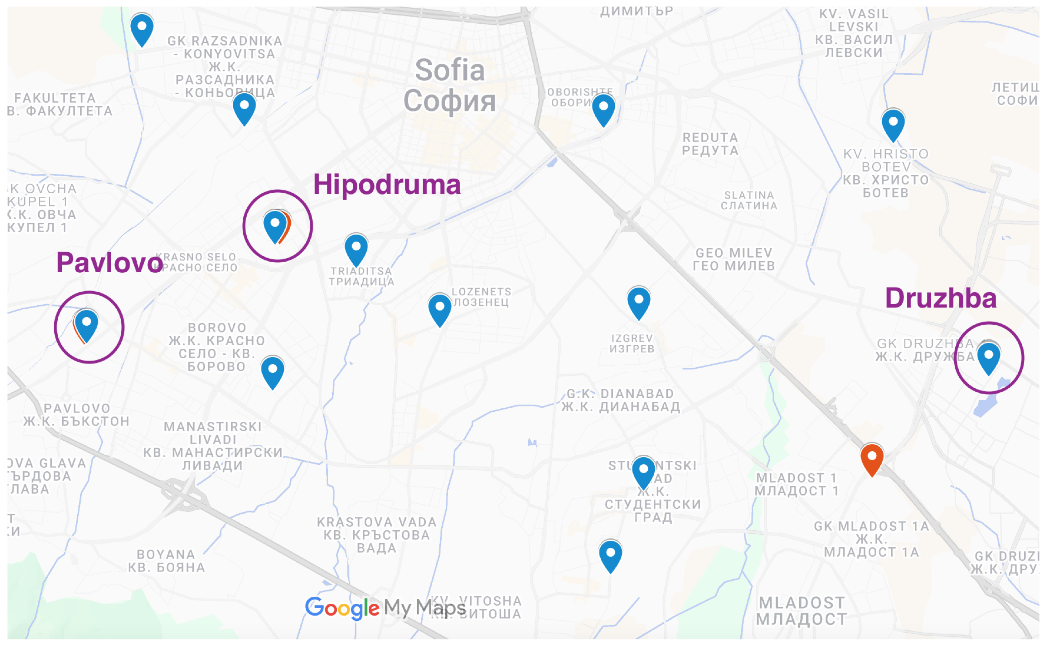
To ensure the accuracy of low-cost air quality sensors, a calibration procedure was performed using an artificial neural network (ANN) approach. The selected stations, Druzhba, Pavlovo, and Hipodruma, were positioned close to the corresponding official monitoring stations, with distances not exceeding a few meters. They can be seen in Figure 1. Given their placement, all three stations were exposed to identical environmental conditions, ensuring a direct comparison between the reference and low-cost sensor measurements.

The calibration process employed a multilayer perceptron (MLP) model to correct the raw particulate matter (PM) readings from low-cost sensors, see Figure 1. The MLP model was chosen due to its effectiveness in regression tasks involving continuous variables. Input features included humidity, atmospheric pressure, temperature, and raw PM measurements obtained from low-cost sensors. The network was trained to predict corrected PM values that closely matched the reference data from official monitoring stations.

The MLP architecture consisted of two hidden layers with 64 and 32 neurons, respectively, utilizing ReLU activation functions. The output layer contained a single neuron with a linear activation function, suitable for continuous value prediction. Model training followed an 80–20% data split, with 80% of the dataset used for training and 20% reserved for testing.

Prior to calibration, the correlation coefficients between the low-cost sensors and the official monitoring stations for PM₁₀ varied significantly across locations. Druzhba exhibited a relatively strong correlation (0.75), while Hipodruma reported poor agreement (0.29) and Pavlovo showed a moderate correlation (0.50). The cause of Hipodruma’s low initial correlation remains unclear, though humidity was found to exert the highest impact on sensor readings compared to atmospheric pressure and temperature. After applying ANN-based calibration, the reliability of low-cost sensor data improved significantly, with the $R^2$ values reaching 0.95, 0.88, and 0.92 for Druzhba, Hipodruma, and Pavlovo, respectively, as shown in

Table 2. Correlation and $R^2$ values for PM₁₀ before and after calibration.

Station	Pre-Calibration Correlation	Post-Calibration ${\mathit{R}}^2$
Druzhba	0.75	0.95
Hipodruma	0.29	0.88
Pavlovo	0.50	0.92

.

Model performance was evaluated using MSE and mean absolute error MAE to quantify the reduction in prediction error after calibration. Additionally, an external validation approach was implemented using a holdout set of unseen data to assess the model’s generalization ability. The results are presented in

Table 3. Correlation and $R^2$ values for PM_2.5 before and after calibration.

Station	Pre-Calibration Correlation	Post-Calibration ${\mathit{R}}^2$
Hipodruma	0.23	0.87

. They demonstrate consistency with the findings from Zhivkov et al. [13], where a similar ANN-based calibration method applied to a different low-cost sensor system achieved comparable improvements in measurement accuracy.

Beyond improving correlation, the ANN calibration framework addressed the data gaps present in both the low-cost and official monitoring systems. Extended periods of missing data—spanning entire days in some cases—were reconstructed using the trained model, effectively restoring continuity in the datasets.

3.2. Spatial Extrapolation of Calibration Parameters

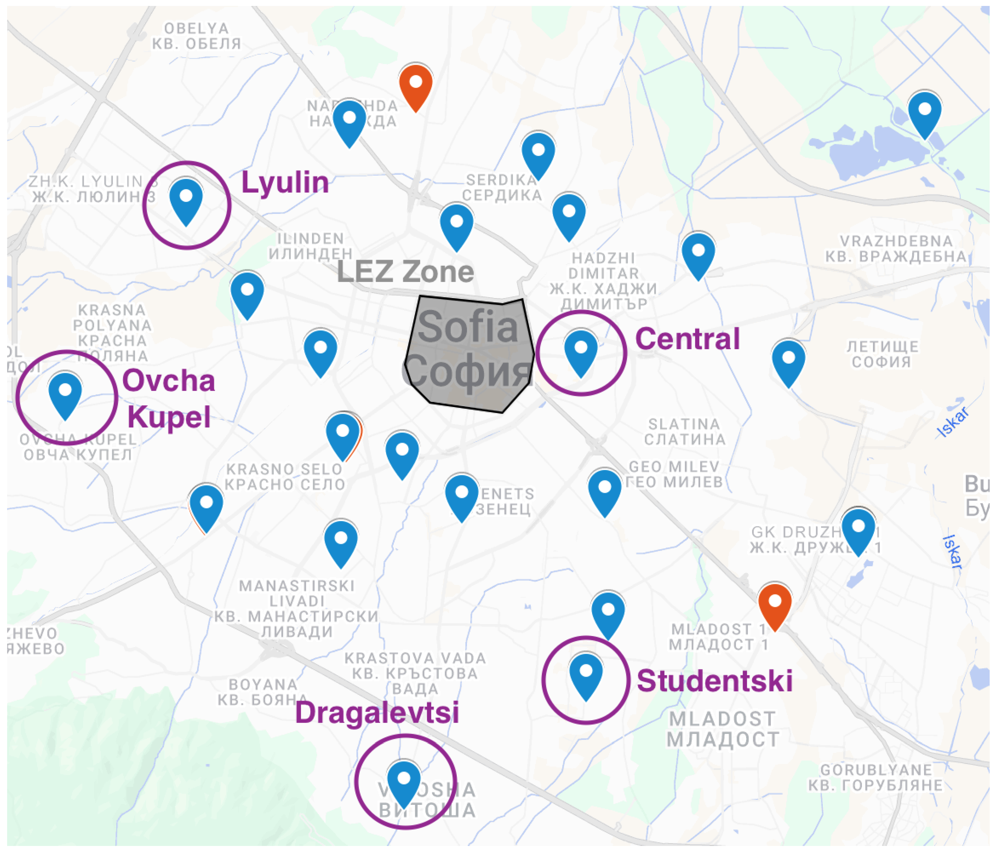
The spatially weighted regression model successfully extended calibration benefits to all 19 uncalibrated stations, with varying degrees of accuracy based on station location and environmental conditions.

Table 4. Calibration performance metrics for selected stations across Sofia, PM₁₀.

Location	Urban Context	Pre-Calibr. ${\mathit{R}}^2$	Post-Calibr. ${\mathit{R}}^2$	RMSE Reduction
Ovcha Kupel	Residential	0.35	0.83	68%
Dragalevtsi	Suburban	0.32	0.79	63%
Central Sofia	Urban Core	0.48	0.91	72%
Studentski	Residential	0.41	0.87	70%
Lyulin	Mixed Use	0.39	0.84	65%

shows calibration performance indicators for stations in various urban environments in Sofia. Calibration efficiency is measured using the $R^2$ between the expected and reference values and the reduction in RMSE compared to uncalibrated measurements.

Stations near the urban core had the highest post-calibration accuracy ($R^2$ = 0.91), possibly due to proximity to the Hipodruma reference station and similar urban topography. Suburban stations like Dragalevtsi demonstrated modest but significant gains ($R^2$ = 0.79), illustrating the durability of the calibration transfer approach across varied urban contexts. The spatial distribution of calibration parameters indicated substantial patterns associated with urban shape and local emission sources. The regional variance in humidity influences coefficients across the monitoring network, emphasizing the greater sensitivity of sensor readings to humidity in locations with higher building density and lower air circulation.

Ovcha Kupel and Dragalevtsi stations consistently had the highest PM₁₀ concentrations following calibration, with mean levels of 59.3 μg/m³ and 56.8 μg/m³, respectively. These increased concentrations connect with local characteristics, including

• Ovcha Kupel has proximity to both the ring of Sofia and the poorest neighborhood of Fakulteta.
• The proximity to domestic heating with wood and coal burning both in Dragalevtsi and Ovcha Kupel.
• Limited public transportation options lead to increased use of private vehicles.
• Street canyon effects that minimize pollutant dispersal.

The polygonal cross-validation method confirmed the stability of the calibration transfer over the monitoring network. When linking stations on a closed polygon route and propagating the calibration parameters sequentially, the median calibration drift ($\Delta$) was 0.057, with 90% of stations having $\Delta$ < 0.08. This small drift suggests that the calibration parameters stayed constant even after passing through several intermediate sites.

The calibration drift was positively correlated with polygon perimeter length (r = 0.62), indicating that spatial distance remained a barrier to calibration transfer. However, including environmental similarity into the weighting function greatly reduced this effect, as indicated by a 37% reduction in calibration drift when compared to a distance-only weighting technique.

The network-wide calibration allowed for a more precise estimate of PM concentration patterns in Sofia. During the study period, 73% of the city area exceeded the PM₁₀ EU limit value (50 μg/m³) on at least one day, compared to 52% in the uncalibrated dataset. This conclusion emphasizes the significance of correct sensor calibration in regulatory compliance evaluation and public health protection measures.

3.3. Temporal Trends and Traffic Impact on PM_2.5 Concentrations

The analysis of temporal variations in particulate matter (PM) concentrations was conducted by comparing pollution levels during high-traffic and low-traffic periods over the course of the measurement campaign. The mobile sensor campaign took place between February 10 and March 1, coinciding with the latter part of the stationary monitoring period. Mobile sensors recorded data at a high frequency of one-second intervals, allowing for a fine-grained temporal analysis of PM fluctuations. The study focused on two distinct traffic conditions: high-traffic periods (8:00 AM–9:30 AM, corresponding to morning rush hour) and low-traffic periods (10:30 AM–12:00 PM). Nighttime measurements were not included in this study.

The results revealed significant differences in PM concentrations between high-traffic and low-traffic periods, as well as between weekdays and weekends. Peak PM levels were consistently recorded during rush hour, indicating a strong influence of vehicular emissions on air quality. In contrast, during late morning hours when traffic density was lower, PM concentrations exhibited a noticeable decline. The difference between weekday and weekend pollution levels further supports the correlation between vehicular activity and PM emissions, with weekends generally showing reduced concentrations due to lower commuting volumes.

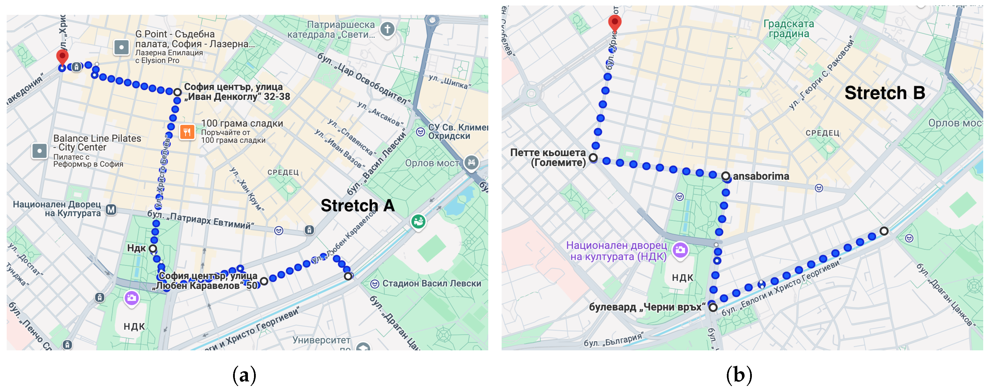
Mobile measurements were conducted along two routes with identical starting and ending points but different paths through the city center. As illustrated in Figure 2, Stretch A follows smaller residential streets and passes through a park area, while Stretch B follows dedicated cycling lanes and runs closer to multi-lane boulevards and bigger interconnections. Both routes traverse areas within and outside the LEZ. Mobile measurements are taken in both directions (start point–finish point and finish point–start point) to avoid bias.

A direct comparison of PM_2.5 values measured by the mobile sensors and the stationary European Environment Agency (EEA) reference station in Sofia is presented in

Table 5. Comparison of PM_2.5 concentrations (μg/m³) between mobile sensors and the stationary EEA monitoring station.

Route	Min	Max	Mean	Stationary (EEA)
Stretch A—rush hour	17	40	21	21.76
Stretch B—rush hour	17	51	25	21.76
Stretch A—low traffic	12	28	16	15.11
Stretch B—low traffic	11	36	17	15.11
Stretch A—weekend	6	14	9	9.39
Stretch B—weekend	7	14	9	9.39

. Measurements were taken simultaneously, allowing for an assessment of how pollution levels varied spatially across different road types and traffic conditions.

The results highlight significant variability in PM_2.5 concentrations across different traffic conditions. During heavy traffic periods (rush hour), the mobile sensor measurements recorded higher peaks than the stationary reference station, reflecting localized pollution spikes due to vehicle emissions. However, during low-traffic hours and weekends, PM concentrations measured along the mobile routes were closer to those recorded by the EEA station, suggesting that background pollution levels dominate in the absence of heavy traffic.

Spatial analysis indicated that pollution spikes were particularly pronounced on major highways, while smaller streets and residential areas exhibited lower PM levels. Pedestrian areas, parks, and designated low-emission zones (LEZs) did not show statistically significant differences in pollution levels; however, further investigation is required to confirm the long-term impact of LEZ policies on air quality. These findings suggest that traffic emissions remain the primary contributor to urban air pollution, with localized variations depending on road type and vehicle density.

The results of this study align with previous findings by [14], who conducted mobile PM measurements in Sofia using a different but comparable sensor system. Although their study focused on different research objectives, both investigations demonstrate the efficacy of mobile sensing in capturing real-time pollution variations at a fine spatial resolution. Notably, no other studies using mobile PM devices have been reported for Sofia, making this research one of the first to provide high-frequency traffic-related pollution insights for the city.

3.4. Spatial Distribution of PM Concentrations

The HSGNN described in the methodology was implemented to analyze pollution dispersion patterns across Sofia’s urban environment. The model integrated data from three sources, mobile sensors, Sofia Municipality low-cost stations, and European Environment Agency reference stations, creating a comprehensive representation of the urban air quality landscape.

The HSGNN successfully captured complex spatiotemporal relationships in PM concentrations by leveraging its multi-scale architecture. The model’s spatial attention mechanism (Equation (4)) was particularly effective at identifying pollution hotspots along major traffic corridors, with the highest attention weights consistently assigned to nodes representing intersections and multi-lane boulevards. This finding aligns with the understanding that these locations experience the highest traffic volumes and, consequently, the greatest emissions from mobile sources.

Temporal analysis revealed that the model’s attention patterns varied significantly between peak and off-peak hours, with a stronger focus on traffic-related nodes during rush hours (8:00 AM–9:30 AM). During low-traffic periods, the attention distribution became more uniform across the urban graph, suggesting that background pollution and non-traffic sources gained relative importance.

Source attribution analysis, performed by backtracking the highest gradient paths in the attention maps, provided insights into pollution origins.

Table 6. Estimated contribution of pollution sources.

Location	Traffic Emissions	Resuspension	Other Sources
Multi-lane Boulevard	65%	25%	10%
Residential Street	30%	50%	20%
Pedestrian Zone	15%	35%	50%
Intersection	70%	20%	10%
Park Area	10%	20%	70%
Underpass	55%	30%	15%

presents the estimated contribution of different emission sources to PM_2.5 concentrations across various urban zones, as determined by the HSGNN model.

The HSGNN model identified significant variations in pollution source contributions across different urban environments. High-traffic areas such as multi-lane boulevards and intersections showed vehicle emissions as the dominant contributor (65–70%), while residential streets exhibited higher contributions from road dust resuspension (50%). In contrast, parks and pedestrian zones showed a more balanced distribution of sources, with greater influence from background and natural sources. Wind speed emerged as a critical factor in pollution dispersion, with the model revealing a strong inverse relationship ($R^2$ = 0.72) between wind speed and PM_2.5 concentrations. The spatial attention mechanism identified that areas with restricted airflow, particularly street canyons and underpasses, tended to accumulate higher pollutant levels even during periods with moderate traffic.

To quantify the value added by mobile sensors, we conducted an ablation study comparing the full HSGNN model against a version trained only on stationary data. The inclusion of mobile sensor data reduced prediction error (RMSE) by 32% and improved hotspot identification precision by 28%, highlighting the importance of high-resolution mobile measurements in capturing fine-grained pollution patterns.

The model’s analysis of urban features revealed that pedestrian zones, parks, and smaller streets exhibited significantly lower PM pollution levels compared to high-traffic areas. Green spaces demonstrated a consistent 30% reduction in PM_2.5 concentrations relative to the surrounding roads, supporting their role in improving urban air quality. Statistical analysis using paired t-tests revealed a moderate but statistically insignificant reduction in PM concentrations within low-emission zones compared to similar road types outside these zones (10% reduction, p = 0.12), though longer-term data will be needed to fully assess their impact. The observed 10% reduction (95% CI: −3% to 22%) is not statistically distinguishable from zero. We cannot conclude with confidence that LEZs produced measurable air quality improvements during our study period.

Figure 3 illustrates the distribution of PM_2.5 concentrations across different urban zones based on the HSGNN model’s predictions, clearly demonstrating the significant variations in pollution levels between high-traffic and low-traffic areas.

3.5. Effectiveness of Low-Emission Zones (LEZs)

Low-emission zones (LEZs) were included in both examined routes; however, the analysis revealed that particulate matter (PM) levels did not differ significantly between areas inside and outside these zones. Instead, the differences in pollution levels were more pronounced between small streets and major boulevards, emphasizing the role of local traffic density rather than the presence of LEZ regulations.

The current LEZ in Sofia enforces restrictions on high-emission vehicles, banning diesel cars registered before 1 January 2007 and gasoline cars registered before 1 January 1998. Violators of this regulation face fines starting at EUR 25. In the three months following the zone’s implementation, 2991 administrative and criminal procedures were initiated, see Figure 4. Before the introduction of the restriction, approximately 20,000 vehicles from the lowest two eco categories (categories 1 and 2) entered the city center daily. On the first day of enforcement (1 December 2024), 4243 violations were recorded. Although the number of violations gradually decreased after initial fines were imposed, more than 2000 high-emission vehicles per day continued to enter the LEZ by the end of February 2025. The highest number of daily violations in this period was recorded on 14 February 2025. However, the relatively low number of fines issued in comparison to the recorded violations raises questions regarding enforcement effectiveness.

Table 7. Comparison of PM_2.5 concentrations (μg/m³) between mobile sensor measurements in the LEZ, non-LEZ areas, and the stationary EEA monitoring station.

Route	Mean LEZ	Mean Non-LEZ	Stationary
Stretch A—heavy traffic	21	21	21.76
Stretch B—heavy traffic	24	25	21.76
Stretch A—low traffic	15	16	15.11
Stretch B—low traffic	16	17	15.11
Stretch A—weekend	9	9	9.39
Stretch B—weekend	9	9	9.39

shows that the reduction in PM levels within the LEZ was minor and statistically insignificant when compared to non-LEZ areas. Although PM concentrations inside the LEZ showed slight improvements, these reductions were insufficient to ensure compliance with all legal air quality standards, particularly on days with high PM levels recorded by stationary monitoring stations. In contrast, studies in cities such as Berlin, Munich, and Madrid have demonstrated that LEZs can significantly lower PM₁₀ and PM_2.5 concentrations, particularly when accompanied by stricter emissions policies and additional measures such as heavy-duty vehicle transit bans [15,16]. For example, in Madrid, the implementation of an LEZ led to measurable declines in PM pollution, although these reductions also fell short of achieving full compliance with air quality regulations [16].

4. Discussion

The twin-based digital framework of this study provides valuable insights into the dynamics of urban mobile emissions in Sofia, Bulgaria. We developed a comprehensive approach to monitoring and analyzing particulate matter concentrations across the urban landscape by integrating multiple data sources with varying degrees of spatial and temporal resolution.

4.1. Main Findings

Our investigation generated some important discoveries. The two-step machine learning calibration approach enhanced the accuracy of low-cost municipal sensors, raising $R^2$ values from 0.29 to 0.87–0.95 following calibration. This demonstrates the potential of employing calibrated low-cost sensors to expand monitoring networks while preserving measurement accuracy.

Second, the mobile sensor program revealed significant geographical and temporal variability in PM concentrations that would have gone undetected with solely stationary monitoring equipment. PM_2.5 levels ranged up to 300% over short distances, with the highest concentrations measured in large multi-lane boulevards during peak traffic hours. This research highlights the limits of typical monitoring networks in detecting localized pollution incidents and exposure dangers.

The GNN model successfully characterized pollution dispersion patterns and identified primary emission sources. Vehicle emissions account for approximately 65% of PM_2.5 concentrations along high-traffic corridors, while road dust resuspension plays a more significant role in residential areas. The observed 30% reduction in PM levels in urban green spaces indicates vegetation’s moderating effect on air pollution.

Fourth, our evaluation of the effectiveness of low-emission zones found that they had no impact on air quality during the initial implementation period. The small difference in PM concentrations between LEZ and non-LEZ locations shows that the current enforcement procedures and scope may be insufficient to accomplish significant air quality improvements.

4.2. Contextual Relevance

Our findings align with several key studies in the field of urban air quality monitoring. The significant spatial variability in PM concentrations observed in our study corroborates research by [17], who similarly documented substantial heterogeneity in urban pollution levels using mobile monitoring systems. The calibration approach we employed builds upon the methodologies developed by [13], who achieved comparable improvements in measurement accuracy through machine learning techniques.

However, our results diverge from those reported by [18], who found more substantial air quality improvements following LEZ implementation in several European cities. This discrepancy may be attributed to differences in enforcement stringency, zone size, or baseline vehicle fleet composition. Our findings more closely resemble those of [19], who observed the modest impacts of Madrid’s LEZ during its initial implementation phase. The observed relationship between green infrastructure and reduced PM concentrations supports an emerging consensus on the role of urban vegetation in mitigating air pollution. Our quantification of this effect (30% reduction) falls within the range reported by [20], who documented PM reductions of 20–40% in various urban green spaces.

4.3. Limitations

Despite the robust methodology used, several limitations warrant consideration. First, the mobile measurement campaign was conducted relatively briefly (10 February to 1 March 2025), which may not capture seasonal variations in pollution patterns. Winter conditions in Sofia typically feature higher pollution levels due to additional residential heating emissions, potentially obscuring the specific contribution of mobile sources.

Second, while our sensor network provided extensive spatial coverage of the city center, peripheral areas and industrial zones were underrepresented. This sampling bias may affect the generalizability of our findings to the broader urban area. Additionally, the mobile routes primarily covered daytime hours (8:00 AM–12:00 PM), limiting our understanding of nighttime pollution dynamics.

Third, the calibration approach was based on co-location with reference equipment at only three sites, which may not account for spatial changes in sensor performance across diverse microenvironments.

Fourth, while the GNN model is effective at capturing spatial relationships, it is fundamentally restricted by the quality and completeness of the input data. Traffic density estimates are based on municipal traffic monitoring systems that may not account for all vehicle kinds or temporary traffic situations.

Finally, our assessment of LEZ effectiveness was conducted only three months after its introduction, which may be insufficient to detect long-term behavioral changes or changes in fleet composition in response to the policy.

4.4. Clinical and Practical Usefulness

The findings from this study have several important implications for urban planning, environmental policy, and public health. First, the significant variation in PM exposure along different urban routes highlights the need for more nuanced approaches to transportation planning. For example, the placement of cycling infrastructure along major roads may inadvertently increase cyclist exposure to harmful pollutants, suggesting that alternative routes through lower-traffic areas could produce health benefits.

Second, the demonstrated effectiveness of urban vegetation in reducing PM concentrations provides empirical support for green infrastructure initiatives. Urban planners can use these findings to strategically integrate parks and street trees in areas of high pollution to mitigate exposure risks.

Third, the limited effectiveness of the current LEZ implementation provides useful lessons for policy refinement, and additional policies and infrastructure improvements should be considered to achieve greater effectiveness. Currently, the city lacks a stationary air quality monitoring station to assess long-term air pollution trends and there are insufficient public charging stations for electric vehicles in key parking areas and few incentives for low-emission vehicle owners. To fill these gaps, we recommend the installation of at least two municipal air quality monitoring stations: one on a major boulevard with heavy traffic within the LEZ and another in a pedestrian area around Vitosha Street. These measures, along with stronger enforcement and incentive-based policies, could significantly enhance the effectiveness of Sofia’s LEZ in reducing air pollution.

Fourth, the calibration framework developed in this study offers a cost-effective approach to expanding air quality monitoring networks using low-cost sensors. This methodology can be readily adapted by municipalities facing budget constraints but seeking comprehensive air quality data.

Finally, the digital twin architecture offers a template for integrating heterogeneous data sources into a cohesive analytical framework. This approach can inform long-term urban development strategies, public health advisories during pollution events, and real-time traffic management decisions.

4.5. Future Research Directions

Several avenues for future research emerge from this study. An extended mobile measurement campaign spanning multiple seasons would provide insights into the temporal stability of the observed pollution patterns. Expanding mobile routes to include industrial areas, suburbs, and varied urban morphologies would enhance the spatial representativeness of the findings. Further refinement of the GNN model to incorporate additional variables, such as building height, street canyon configurations, and detailed vehicle fleet composition, could improve predictive accuracy. The integration of citizen science approaches and personal exposure monitoring would add valuable dimensions to the analysis.

An essential topic for further research is the long-term monitoring of LEZ effectiveness as the composition of the fleet changes and the enforcement improves. Best practices for policy design may be found through comparative studies conducted in several towns with different LEZ implementations.

Lastly, employing epidemiological methods to investigate the connection between simulated pollution exposure and health consequences would increase this research framework’s applicability to public health.

5. Conclusions

This study introduced a digital twin-based framework for the real-time monitoring and analysis of urban mobile-source emissions. The digital twin in this context is defined as a dynamic, data-driven representation of the urban air quality system, integrating real-time data from various sources, advanced computational models, and machine learning algorithms to simulate and predict air quality conditions.

The digital twin framework proposed in this study consists of several key components, including real-time data integration that incorporates information from environmental sensors, meteorological forecasts, traffic flow patterns, and industrial emission outputs; advanced computational models that utilize machine learning algorithms and simulation tools to process and analyze the integrated data; predictive modeling that generates models capable of anticipating future air quality trends and potential hazards; and decision support that provides actionable insights for policymakers, urban planners, and environmental regulators to make informed decisions.

The real prototype of the digital twin in this study is the urban air quality monitoring system deployed in Sofia, Bulgaria, which integrates data from fixed reference stations, low-cost municipal sensors, and mobile measuring devices to create a dynamic and accurate representation of the air quality conditions in the city.

Despite its advantages, the framework has certain limitations. The accuracy of predictions depends upon the quality and availability of input data, and computational demands may limit real-time scalability in large urban areas. Future research should focus on optimizing data integration methods, enhancing model interpretability, and expanding the framework’s applicability to various environmental scenarios.

In conclusion, this work contributes to the advancement of digital twin applications in environmental science by providing a robust, data-driven approach for air quality monitoring. Further developments in machine learning, sensor technologies, and cloud computing are expected to refine the system, making it more efficient and accessible for real-world deployment.