Influence of Clouds and Aerosols on Solar Irradiance and Application of Climate Indices in Its Monthly Forecast over China

Abstract

Based on the Clouds and the Earth’s Radiant Energy System (CERES) satellite data from 2001 to 2023 and the climate indices from the National Oceanic and Atmospheric Administration (NOAA), this study analyzes the solar irradiance over mainland China and the impacts of clouds and aerosols on it and constructs monthly forecasting models to analyze the influence of climate indices on irradiance forecasts. The irradiance over mainland China shows a spatial distribution of being higher in the west and lower in the east. The influence of clouds on irradiance decreases from south to north, and the influence of aerosols is prominent in the east. The average explained variance of clouds on irradiance is 86.72%, which is much higher than that of aerosols on irradiance, 15.62%. Singular Value Decomposition (SVD) analysis shows a high correlation between the respective time series of irradiance and cloud influence, with the two fields having similar spatial patterns of opposite signs. The variation in solar irradiance can be attributed mainly to the influence of clouds. Empirical Orthogonal Function (EOF) analysis indicates that the variation in the first mode of irradiance is consistent in most parts of China, and its time coefficient is selected for monthly forecasting. Both the traditional multiple linear regression method and the Long Short-Term Memory (LSTM) network are used to construct monthly forecast models, with the preceding time coefficient of the first EOF mode and different climate indices as input. Compared with the multiple linear regression method, LSTM has a better forecasting skill. When the input length increases, the forecasting skill decreases. The inclusion of climate indices, such as the Indian Ocean Basin (IOB), El Nino–Southern Oscillation (ENSO), and Indian Ocean Dipole (IOD), can enhance the forecasting skill. Among these three indices, IOB has the most significant improvement effect. The research provides a basis for accurate forecasting of solar irradiance over China on monthly time scale.

1. Introduction

With the progress of society, there is a continuous growth in the demand for energy. However, traditional fossil fuels pose environmental hazards and can no longer fully meet the developmental needs of human society [1]. As a zero-emission clean energy source, photovoltaic power generation has been widely developed and utilized. Notably, solar irradiance directly impacts the power generation efficiency of photovoltaic systems [2]. In this study, solar irradiance refers to the all-sky shortwave radiation that reaches the ground, composed of both direct and diffuse components. Its accurate estimation is crucial for solar radiation budget studies and the photovoltaic industry [3,4,5]. The Chinese mainland exhibits exceptional solar energy potential, receiving annual solar irradiance corresponding to 170 billion tons of coal equivalent [6].

Ground-based solar irradiance observation stations in China are sparse and unevenly distributed [7]. When analyzing spatial features of solar irradiance, spatial interpolation is often employed, though the method can introduce significant errors. Satellite observations, with their uniform spatial coverage, can effectively overcome this limitation (e.g., sparse ground stations). This study utilizes high-accuracy irradiance data from the Clouds and the Earth’s Radiant Energy System (CERES) to analyze the spatial patterns of solar irradiance and its interannual variation. The multiple linear regression (MLR) model and Long Short-Term Memory (LSTM) network are used to construct monthly forecast models for solar irradiance.

Variations in irradiance are primarily influenced by cloud cover and aerosols [8], which are affected by atmospheric circulation and other factors. Zhao et al. [9] analyzed the interactions among eight major climate indices and their corresponding climate modes, along with their global climatic impacts. This study selects climate indices from Zhao et al.’s study [9] to forecast irradiance over mainland China. Key climate indices, including ENSO, IOB, and IOD, are incorporated to account for their known impacts on East Asian climate anomalies [10]. ENSO, as the strongest interannual climate variability signal, has great impact on the Asian monsoon and global atmospheric circulation. During El Niño years, the South Asian summer monsoon weakens, reducing moisture transport to East Asia and leading to decreased precipitation in northern China [11]. In La Niña development years, anomalous East Asian summer monsoons can trigger flooding events in the Yangtze and Yellow River basins, as well as in South Korea and Japan [12]. Sea surface temperature variations in the Indian Ocean are mainly characterized by two independent modes: the basin-wide uniform anomaly pattern (IOB) and the east–west dipole pattern (IOD) [13]. The IOB can induce a secondary warming effect, exciting an anomalous anticyclone over the northwestern Pacific, which delays the onset of the South China Sea monsoon but intensifies it, thereby increasing precipitation in southern China [14]. The IOD can enhance precipitation north of the Yangtze River while causing drier conditions in southern China [15] and also affect precipitation along a diagonal zone spanning from Yunnan Province to the Korean Peninsula [16]. Abnormal precipitation patterns can lead to anomalous cloud cover, ultimately impacting solar irradiance. Including climate indices in the predictive models of solar irradiance over China can potentially enhance the forecasting skill of these models.

Current irradiance forecasting methods primarily include statistical approaches based on historical irradiance data [17] and physical approaches relying on atmospheric variables such as cloud cover and temperature [18]. These methods typically focus on short-term forecasts (hours to days) or synoptic time scale forecasts (7–10 days). Monthly irradiance forecasting would greatly benefit long-term power grid scheduling and planning. This study applies key climate indices as predictors, focusing on monthly forecasting.

Based on CERES satellite data and climate indices from 2001 to 2023, this study quantifies cloud and aerosol effects on surface irradiance over mainland China. The multiple linear regression model and Long Short-Term Memory network are used to forecast monthly solar irradiance and analyze the impact of climate indices on the forecast. After the introduction, Section 2 describes the data and methodology. Section 3 examines the spatial characteristics of solar irradiance over China and quantifies the impact of clouds and aerosols on solar irradiance, using Empirical Orthogonal Function (EOF) analysis to extract the time coefficient of the first EOF mode for the monthly forecast. Section 3 also compares LSTM and multiple linear regression models in terms of monthly irradiance forecasting and investigates the influence of climate indices when included in these forecast models. Section 4 discusses some limitations of our research, and Section 5 summarizes our research.

2. Data and Methods

2.1. Data

The irradiance data used in this study were obtained from the CERES_SYN1deg_Edition4.1 dataset, acquired by the National Aeronautics and Space Administration (NASA) through CERES sensors aboard the Terra and Aqua environmental satellites (http://ceres.larc.nasa.gov/order_data.php, accessed on 26 October 2024) [19], with a spatial resolution of 1° × 1°. Monthly surface irradiance data for mainland China from January 2001 to December 2023 were extracted from the dataset, which includes irradiance values under clear-sky (no clouds), all-sky, clear-sky and no-aerosol, and all-sky no-aerosol conditions. Compared to other satellite data and reanalysis datasets, CERES data are closer to ground station observations [20,21].

Six climate indices were selected based on their established roles in modulating precipitation and cloud cover over China, which are critical drivers of solar irradiance variability (Table 1). These include the ENSO, IOD, Atlantic Meridional Mode (AMM), and Pacific Meridional Mode (PMM), obtained directly from monthly datasets provided by NOAA (https://psl.noaa.gov/data/climateindices/list/, accessed on 11 October 2024). The remaining two indices (IOB and SIOD) were derived from NOAA’s Extended Reconstructed SST V5 dataset [22], with a global monthly mean SST at 2° × 2° resolution. All indices span the period from January 2001 to December 2023.

Table 1. Climate indices used for their potential impact on monthly solar irradiance forecast over China.

Index	Definition
IOD	SST anomaly difference between the western (50–70° E, 10° S–10° N) and eastern (90–110° E, 10–0° N) tropical Indian Ocean
SIOD	SST anomaly difference between the south-central (65–85° E, 25–10° S) and southeastern (90–120° E, 30–5° S) Indian Ocean
IOB	Area-averaged SST anomaly over the Indian Ocean (20° S–20° N, 40–110° E)
ENSO	SST anomaly in the Niño 3.4 region (5° N–5° S, 120–170° W)
AMM	Leading mode of maximum covariance analysis for SST and 10 m winds over the Atlantic (21° S–32° N, 74° W–15° E)
PMM	Analogous to AMM but for the Pacific basin

This study utilizes rigorously quality-controlled CERES SYN1deg Edition 4.1 satellite radiation data and NOAA climate index datasets. Prior to release, these datasets underwent systematic quality assurance procedures at the source institutions, including standardized processing such as outlier detection, spatiotemporal consistency checks, and cross-validation [19,22].

2.2. Quantifying the Influence of Cloud and Aerosol on Solar Irradiance

Following Ramanathan’s definition [23], cloud-induced irradiance attenuation is calculated as the difference between clear-sky and all-sky irradiance. Similarly, aerosol-induced attenuation is computed as the difference between pristine and clear-sky irradiance. Both definitions are explicitly specified in the CERES dataset documentation (https://ceres.larc.nasa.gov/documents/DQ_summaries/CERES_SYN1deg_Ed4A_DQS.pdf, accessed on 26 October 2024). Consequently, the difference between pristine and all-sky irradiance equals the combined effects of clouds and aerosols on irradiance:

$$F_{cloud}=F_{clear}-F_{all}$$

(1)

$$F_{aerosol}=F_{pristine}-F_{clear}$$

(2)

where $F_{cloud}$ is cloud-induced irradiance attenuation; $F_{aerosol}$ is aerosol-induced irradiance attenuation; $F_{clear}$ represents solar irradiance under clear-sky conditions; $F_{all}$ represents solar irradiance under all-sky conditions; and $F_{pristine}$ represents solar irradiance under pristine conditions. All variables have units of W/m².

2.3. Conventional Statistical Method

The study employed the Pearson correlation coefficient (r) and root mean square error (RMSE) to evaluate the prediction model’s accuracy, calculated as follows:

$$r={\displaystyle \frac{{\displaystyle \sum _{\mathrm{t}=1}^N(P_{forecasting}-\overline{P_{forecasting}})(P_{true}-\overline{P_{true}})}}{\sqrt{{\displaystyle \sum _{\mathrm{t}=1}^N{(P_{forecasting}-\overline{P_{forecasting}})}^2{\displaystyle \sum _{t=1}^N{(P_{true}-\overline{P_{true}})}^2}}}}}$$

(3)

$$RMSE=\sqrt{{\displaystyle \frac{{\displaystyle \sum _{\mathrm{t}=1}^N{(P_{forecasting}-P_{true})}^2}}{N}}}$$

(4)

where $P_{forecasting}$ is the predicted value at time t; $P_{true}$ is the observed value at time t; $\overline{P_{forecasting}}$ and $\overline{P_{true}}$ represent the mean values of predicted and observed data; and N is the total number of data samples.

2.4. Random Forest

This study adopted the random forest (RF) algorithm to assess the importance of key factors affecting solar irradiance. As an ensemble learning method, random forest quantifies feature contributions by constructing multiple decision trees and calculating the mean decrease in impurity (Gini importance) during node splitting across all trees, as well as the model accuracy decline after randomly permuting feature values (permutation importance) [24]. Using solar irradiance and six climate indices as input features, we trained a random forest model containing 100 decision trees to output importance scores for each climate index, thereby evaluating the relative contribution of each climate index.

2.5. Singular Value Decomposition

The Singular Value Decomposition (SVD) method essentially performs generalized diagonalization of the cross-covariance matrix between two physical fields. This approach effectively extracts mutually independent coupled modes from the left and right fields, revealing the spatial correlation characteristics of spatiotemporal relationships between the two fields. The decomposed heterogeneous spatial fields clearly demonstrate the association between expansion coefficients of the left (or right) field and temporal variations of the right (or left) field [25]. In this study, the SVD method employs all-sky solar irradiance as the left singular vector and cloud/aerosol effects on radiation as the right singular vector, investigating dominant cloud and aerosol modes influencing solar irradiance over China.

2.6. Empirical Orthogonal Function

Empirical Orthogonal Function (EOF) decomposition was employed to examine interannual variability characteristics of solar irradiance over mainland China and adjacent seas, with the most representative continental time coefficient selected as the predictand for subsequent forecasting. EOF is a widely used multivariate data analysis tool that simplifies complex datasets, first introduced to meteorological research in 1956 and now extensively applied in climate studies [26]. EOF analysis decomposes climate variable fields into products of spatial modes and temporal coefficients. The eigenvectors characterize spatial distribution patterns (spatial modes) that reveal the field’s spatial organization, while principal components represent temporal variations (time coefficients) describing sequential changes of corresponding spatial modes. Linear combinations of different spatial modes and their associated time coefficients can reconstruct the original data field and explain its variance characteristics.

2.7. Long Short-Term Memory Network

The Long Short-Term Memory (LSTM) network is adopted for its demonstrated effectiveness in modeling temporal dependencies in climate data [27]. The key innovation of LSTM lies in its gating mechanism, which effectively addresses the vanishing/exploding gradient problems inherent in traditional RNNs while capturing long-term dependencies in sequential data. For this study, the LSTM model was implemented using the LSTM module from Python’s TensorFlow.Keras. layers, with historical irradiance and climate indices serving as input features.

Within the LSTM unit architecture (Figure 1), there exist three fundamental gating mechanisms that collectively regulate information retention: the input gate, forget gate, and output gate. The input gate selectively determines which input values should be stored in the subsequent cell state. The forget gate modulates the retention of historical state information by identifying obsolete memory content. The output gate controls the propagation of internal state information to external outputs. Figure 1 illustrates the structural composition of these gating mechanisms, where $i$, $f$, and $O$ denote the input gate, forget gate, and output gate, respectively. The symbol $C_{\mathrm{t}}$ represents the current cell state, while $\overline{C}$ indicates the candidate state for subsequent updates.

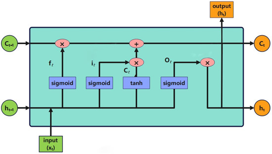
Figure 1. Schematic illustration of LSTM unit.

The LSTM unit computations are governed by the following equations:

$$f_t=\sigma (W_f\ast [h_{t-1},x_t]+b_f)$$

(5)

$$i_t=\sigma (W_i\ast [h_{t-1},x_t]+b_i)$$

(6)

$${\overline{C}}_t=\tanh (W_c\ast [h_{t-1},x_t]+b_c)$$

(7)

$$C_t=f_t\ast C_{t-1}+i_t\ast {\overline{C}}_t$$

(8)

$${\mathrm{o}}_t=\sigma (W_o\ast [h_{t-1},x_t]+b_o)$$

(9)

$$h_t=o_t\ast \tanh (c_t)$$

(10)

where $h_{t-1}$ is the previous unit’s output; $x_t$ is the current unit’s input; $W_i$, $W_f$, $W_o$, and $W_c$ are weight matrices; $b_i$, $b_f$, $b_o$, and $b_c$ are bias vectors; ∗ denotes element-wise matrix multiplication; σ is the sigmoid activation function; and $\tanh$ represents the hyperbolic tangent activation function.

In our previous work, the LSTM method was successfully applied to short-term photovoltaic power prediction. The results demonstrated that incorporating meteorological variables into LSTM models can enhance prediction accuracy [17]. Building upon previous experience for photovoltaic power forecasting, an optimal 8:2 ratio was maintained for training (80%) and test (20%) set division, which had been demonstrated to deliver reasonable performance without significant overfitting.

In this study, the first 18 years of irradiance and climate index data were selected as the training set, while the last 5 years served as the test set. The LSTM network was configured with the mean squared error as the loss function. Various input lengths (1, 3, 6, 9, and 12 months) were tested. The architecture consisted of 2 stacked LSTM layers (50 neurons each), with a dropout layer (rate = 0.2) between them to prevent overfitting. Training proceeded for 50 epochs using the Adam optimizer [28].

When constructing an LSTM model for monthly forecasting, significant dimensional differences among the input variables may adversely affect model training efficiency and prediction accuracy. We performed min–max normalization on all variables prior to model development. The normalization procedure rescales all features to the interval [0, 1] using the following transformation:

$$X_{\mathrm{b}}={\displaystyle \frac{X_a-X_{\min }}{X_{\max }-X_{\min }}}$$

(11)

where $X_a$,$X_{\mathrm{b}}$ represent the original and normalized values, and $X_{\max }$,$X_{\min }$ represent the maximum and minimum values of the variable.

3. Results

3.1. Spatial Characteristics of Solar Irradiance

The spatial distribution of annual mean solar irradiance over mainland China during 2001–2023 shows clear regional differences (Figure 2a), with a pattern of higher values in the northwest and lower values in the southeast. The higher solar irradiance intensities (>200 W/m², peaking at 246 W/m²) are observed in Xinjiang Province and the Tibetan Plateau, attributable to the high altitude, thin atmosphere, and consequently reduced attenuation by clouds and aerosols [29]. Conversely, the Sichuan Basin exhibits the lowest solar irradiance levels (mostly around 140 W/m², with a minimum around 120 W/m²), resulting from its enclosed topography and persistent overcast conditions due to the convergence of warm and cold air masses, which enhance atmospheric scattering and absorption. For better interpretation of the spatial patterns, the corresponding topographic data of China (1:16,000,000 scale) supervised by the Ministry of Natural Resources (Available at: http://bzdt.ch.mnr.gov.cn/index.html, accessed on 3 May 2025) can be referenced to correlate terrain features with the observed solar irradiance distribution.

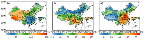
Figure 2. The 2001 to 2023 averaged downward surface shortwave all-sky irradiance over China and the influence of clouds and aerosols on irradiance: (a) all-sky solar irradiance (W/m²); (b) the influence of clouds (W/m²); and (c) the influence of aerosols (W/m²).

Figure 2b quantifies cloud-induced irradiance attenuation, showing a distinct south-to-north decreasing gradient (23–123 W/m²). The strongest attenuation occurs in the precipitation-rich Sichuan Basin and southern coastal regions, while northern areas experience minimal cloud effects (~30 W/m²).

Figure 2c delineates the annual mean spatial distribution of aerosol-induced irradiance attenuation (ranging from 5 to 55 W/m²), exhibiting distinct spatial heterogeneity with elevated values in southeastern regions and diminished values in both western and northern areas. The Tibetan Plateau has minimal attenuation attributable to its elevated topography and low aerosol loading, whereas regions such as the central part of China and eastern China, which are the economically developed and densely populated regions of China, have higher attenuation due to aerosols.

To compare these three components (solar irradiance, influence of clouds, and influence of aerosols), Figure 3 presents their distributions at four representative sites selected from the spatial patterns in Figure 2: point A (29.5° N, 84.5° E) in Tibet with maximum irradiance, point B (28.5° N, 107.5° E) in the Sichuan Basin showing minimum irradiance and maximum cloud effect, point C (40.5° N, 92.5° E) in Xinjiang with minimum cloud effect, and point D (32.5° N, 114.5° E) in eastern China exhibiting maximum aerosol effect.

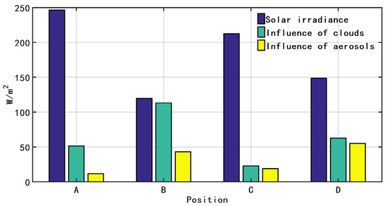
Figure 3. Comparison of solar irradiance, influence of clouds, and influence of aerosols at four representative sites in China (W/m²).

3.2. Influence of Clouds and Aerosols on Solar Irradiance

To elucidate the distinct impacts of clouds and aerosols on solar irradiance, this section quantifies their respective contributions through variance explained analysis. As shown in Figure 4, which uses anomaly data with the climatological seasonal cycle removed, clouds dominate irradiance variability across most regions, explaining 86.72% of the variance on average and exhibiting obvious spatial heterogeneity. While the Bohai Rim region shows relatively lower explained variance of clouds, its explained variance still exceeds 58% (Figure 4a). In contrast, aerosol effects are considerably weaker, with a mean of explained variance of only 15.62% (maximum 52.8%). The explained variance of aerosols is relatively higher in economically developed, densely populated, and heavily industrialized regions, especially North China and the Bohai Rim (Figure 4b). Notably, negative explained variance values over Tibet and Qinghai suggest that aerosols cannot account for irradiance variability. Overall, clouds exert a far greater influence on irradiance than aerosols do.

Figure 4. The explained variance of anomalous solar irradiance by clouds and aerosols: (a) explained variance by clouds (%); (b) explained variance by aerosols (%).

The dominant spatial modes of clouds and aerosols influencing solar irradiance over China were analyzed through Singular Value Decomposition (SVD) analysis, with solar irradiance anomalies selected as the left field and the influence of clouds and aerosols on irradiance as the respective right fields. As the first SVD mode was found to represent the primary variability pattern, accounting for 46.24% and 70.66% of the total variance for cloud and aerosol fields, respectively, the analysis was focused exclusively on this mode.

The SVD spatial modes between solar irradiance and the influence of clouds (Figure 5a,b) show consistent irradiance variation over most of China, except in the northeastern and southwestern regions (Figure 5a). The spatial pattern of the influence of clouds on irradiance (Figure 5b) resembles the irradiance pattern (Figure 5a) but with opposite signs. The temporal expansion coefficients of the left and right fields exhibit a high temporal correlation coefficient of 0.93 (Figure 5c). This further confirms the significant role of cloud effects in irradiance variability.

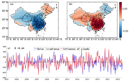
Figure 5. The first mode of Singular Value Decomposition (SVD) analysis of solar irradiance and the influence of clouds on irradiance: (a) irradiance; (b) the influence of clouds; and (c) the temporal expansion coefficients of the two fields.

The SVD analysis of solar irradiance and aerosol influence (Figure 6) demonstrates that aerosol impacts are primarily concentrated in eastern China, particularly the Bohai Rim region. The spatial patterns of irradiance anomalies (Figure 6a) and the influence of aerosols on irradiance (Figure 6b) show opposite signs. The correlation coefficient between their temporal coefficients is only 0.63 (Figure 6c). Notably, all correlation coefficients in Figure 5c and Figure 6c are significant at the 95% level. The SVD results are consistent with the variance explained analysis.

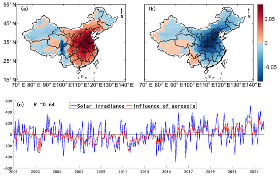
Figure 6. The first mode of SVD analysis of solar irradiance and the influence of aerosols on irradiance: (a) irradiance; (b) the influence of aerosols; and (c) the temporal expansion coefficients of the two fields.

3.3. EOF Analysis of Solar Irradiance

To investigate the interannual variability characteristics of solar irradiance over mainland China and construct monthly forecast models, EOF analysis was performed on solar irradiance anomalies. The EOF analysis of solar irradiance over mainland China reveals that the first five modes collectively account for 53.67% of the total variance (Table 2). The leading mode explains 19.67% of the total variance, significantly exceeding other modes, and passes the North test [30]. Therefore, our analysis focuses on the leading mode, with its temporal coefficients selected as the predictand for monthly-scale forecasting.

Table 2. Variance contribution of the top 5 modes in EOF analysis of solar irradiance over mainland China.

EOF Modes	Variance Contribution/%	Cumulative Variance%
1	19.67	19.67
2	11.87	31.54
3	8.15	36.96
4	7.34	47.03
5	6.65	53.67

The spatial pattern of the first EOF mode for irradiance (Figure 7) exhibits uniform signs over most of China, except for opposite-sign regions in southwestern Tibet, Yunnan Province, and northeastern China. This coherent pattern indicates same-sign irradiance variability over China in the first mode. To test monthly forecast models of solar irradiance instead of irradiance at a particular location, the time coefficient of the first EOF (Figure 7b) is used.

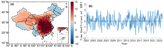
Figure 7. The first mode of EOF analysis of solar irradiance anomalies over China: (a) spatial pattern; (b) time coefficient of the first mode of EOF.

3.4. Monthly Forecast of Solar Irradiance

3.4.1. Application of Climate Indices

The analysis in Section 3.2 indicates that irradiance anomalies are predominantly controlled by clouds, which are closely linked to precipitation. Building on established knowledge of climate indices’ influences on precipitation patterns in China [11,12,14,15,16], this section performs correlation analysis, concurrent multiple linear regression, and random forest assessment (Table 3) between the time coefficient of the first EOF mode of irradiance and representative climate indices to systematically examine their relationships. The multiple linear regression model significantly reproduces the temporal variations of the first EOF mode, which is formulated as:

$$Irradianc{e}_{EOF1}=0.13-0.73\times IOB+0.19\times ENSO+0.14\times IOD+0.1\times AMM+0.08\times SIOD-0.12\times PMM$$

where the intercept (0.13) represents the baseline irradiance level independent of climate influences, and each coefficient quantifies the relative contribution of the corresponding climate index. The correlation coefficient of the predicted time coefficient and the original time coefficient is significant at the 95% level.

Table 3. Correlation coefficients (r), regression coefficients, and importance scores between the time coefficient of the first EOF mode of solar irradiance and the climate indices.

	r	Regression Coefficients	Importance Score
IOD	−0.0059	0.14	0.176
SIOD	0.0495	0.08	0.140
IOB	−0.1802 *	−0.73	0.198
ENSO	−0.0316	0.19	0.177
AMM	0.0949	0.10	0.167
PMM	0.0049	−0.12	0.141

* Significant, with p < 0.05.

The regression coefficients above confirm the dominant influence of IOB, consistent with its top-ranked importance score in random forest analysis. Both multiple linear regression and random forest analyses consistently identified IOB, ENSO, and IOD as the top three influential indices for irradiance (Table 3). Therefore, these three indices were selected to be included as predictors to analyze the influence of climate indices in monthly solar irradiance forecasting.

3.4.2. Comparison of Forecasting Skill

This section systematically evaluates the impacts of climate indices on monthly irradiance forecasting skill. Forecast models were developed using both MLR and LSTM methods, with the preceding time coefficient of the first EOF mode and climate indices as predictors. The potential contributions of the IOB, ENSO, and IOD indices to the forecasting skill were independently quantified by applying them separately in forecasting. Two forecasting schemes were designed: one using only time coefficients as predictors and the other incorporating both time coefficients and climate indices. By comparing these schemes, the impact of introducing different climate indices on irradiance forecasting was investigated. The Pearson correlation coefficient (r) and root mean square error (RMSE) were employed to quantify the discrepancies between model forecasts and actual values.

When the MLR method was applied for forecasting, time coefficients from the preceding 1, 3, 6, 9, and 12 months were selected to forecast the value of the current month. We examined the impacts of different input lengths and predictor combinations on forecasting skill. For instance, when the input length is 3, data from months t − 3, t − 2, and t − 1 are used to construct the MLR model for predicting the irradiance in month t. For the LSTM method, the dataset was split into training and testing sets at an 8:2 ratio. To maintain chronological integrity, the first 18 years of irradiance and climate indices data were designated as the training set, while the last 5 years served as the testing set. Input lengths of 1, 3, 6, 9, and 12 months were tested to explore the predictability of solar irradiance and influence of climate indices.

To assess potential overfitting in the LSTM model with the 8:2 split, a test case was conducted using a 3-month input length and irradiance as the sole predictor (Table 4). Under these conditions, the training set yielded an r of 0.82 and an RMSE of 0.62 between predicted and actual values, while the testing set has an r of 0.83 and an RMSE of 0.69. The negligible difference between training and testing sets indicated no overfitting in this configuration.

Table 4. Performance comparison of LSTM models with 3-month irradiance-only input under different training–testing split ratios.

	8:2		7:3		6:4
	r	RMSE	r	RMSE	r	RMSE
Training set	0.82	0.62	0.81	0.68	0.83	0.65
Testing set	0.83	0.69	0.82	0.73	0.83	0.70

To find out the optimal data partitioning scheme for a monthly time scale, we systematically compared the 8:2, 7:3, and 6:4 splitting ratios. As shown in Table 4, the 8:2 partitioning consistently demonstrated superior performance across all evaluation metrics, exhibiting both a higher r and relatively lower RMSE. It is interesting to note that for short-term forecasting, the 8:2 ratio is also more suitable [17].

Table 5 and Table 6 present the forecasting skill of the MLR and LSTM models, respectively, with varying input lengths and different combinations of climate indices. The relative difference in the r and RMSE between the MLR and LSTM models were calculated and averaged. On average, the r showed a relative improvement of 59.76%, while the RMSE exhibited a relative reduction of 13.12% for LSTM models. Notably, with a 6-month input length, the inclusion of the IOD index alongside irradiance yielded the most significant improvement, with the r increasing from 0.25 to 0.61 (a 144% relative enhancement). For a 3-month input length, the RMSE was reduced from 0.92 to 0.63. Figure 8 compares the forecasts of the LSTM and MLR models with a 1-month input length, with the LSTM model demonstrating higher forecasting skill than the MLR model.

Table 5. Forecasting skill in terms of correlation coefficient and RMSE of the time coefficient of the first EOF mode using MLR model with different input lengths and climate indices.

	Irradiance		IOB and Irradiance		ENSO and Irradiance		IOD and Irradiance
Input Length/Month	r	RMSE	r	RMSE	r	RMSE	r	RMSE
1	0.73	0.68	0.74	0.72	0.67	0.75	0.64	0.78
3	0.51	0.86	0.56	0.86	0.47	0.88	0.38	0.92
6	0.34	0.94	0.44	0.92	0.34	0.94	0.25	0.98
9	0.29	0.95	0.40	0.94	0.27	0.96	0.24	0.97
12	0.28	0.96	0.40	0.94	0.26	0.96	0.23	0.98

Table 6. Forecasting skill in terms of correlation coefficient and RMSE of the time coefficient of the first EOF mode using LSTM model with different input lengths and climate indices.

	Irradiance		IOB and Irradiance		ENSO and Irradiance		IOD and Irradiance
Input Length/Month	r	RMSE	r	RMSE	r	RMSE	r	RMSE
1	0.99	0.55	0.99	0.56	0.98	0.62	0.95	0.62
3	0.83	0.69	0.84	0.63	0.84	0.70	0.84	0.63
6	0.59	0.95	0.66	0.88	0.62	0.93	0.61	0.93
9	0.42	1.05	0.54	1.00	0.51	1.00	0.49	1.00
12	0.37	1.09	0.40	1.08	0.38	1.06	0.27	1.08

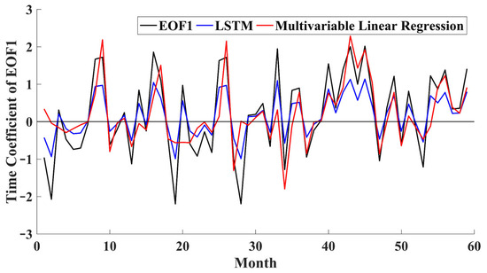
Figure 8. Comparison of forecasts from the LSTM model and the multiple linear regression (MLR) model against the time coefficient of the first EOF mode with 1-month input.

Analysis of both the MLR and LSTM models revealed that as the input length was increased, both forecasting schemes—using irradiance alone or combining climate indices with irradiance—exhibited a gradual decline in the r and a rise in RMSE. This suggests that current irradiance is closely tied to recent historical data (e.g., 1 or 3 months). Both the MLR and LSTM models can effectively capture short-term temporal dependencies [31]. However, when longer input lengths were involved, the introduction of climate indices can improve forecasting skill compared to using irradiance alone.

For the LSTM method, all three climate indices—IOB, ENSO, and IOD—were found to contribute to improved forecasting skill to varying degrees. Compared to the irradiance-only model, the model with both IOB indices and irradiance achieved an average relative r improvement of 9.95% and an average RMSE reduction of 3.99%. By including the ENSO index, the LSTM model can improve the forecasting skill for input lengths of 6, 9, and 12 months, delivering an average relative r increase of 9.74% and an average RMSE decrease of 3.21%. By including the IOD index, the LSTM method exhibited improvements for input lengths of 3, 6, and 9 months, with an average relative r increase of 7.08% and an average RMSE reduction of 5.19%.

4. Discussion

4.1. CERES Data Validation

The spatial characteristics of the influence of clouds on irradiance (Figure 2b) corroborate Qin’s research [32]. While Qin’s research has utilized irradiance data from the CERES_SYN dataset (2001–2018) [32], this research employs the latest updated version (released April 2021) and quantifies the influence of clouds and aerosols on solar irradiance.

Extensive validation has confirmed that although CERES data have a spatial resolution of 1°, their radiation retrieval accuracy in China is significantly better than that of other available data sources [20,21]. Systematic validation studies show that obtaining high-quality ground-based radiation observations faces numerous challenges: national-level radiation observation stations (such as the 91 CMA stations used in [21]) are sparsely distributed, and acquiring continuous multi-year complete observation data encounters administrative and technical barriers. The validation by [21] during 2011–2018 demonstrated that the CERES SYN1deg product achieves a correlation coefficient of 0.955 (RMSE = 20.042 W/m²) with ground observations at monthly scales, indicating its accuracy fully meets the requirements for regional climate research. Particularly in key regions like the Tibetan Plateau, CERES data effectively overcome the limitation of scarce ground stations by providing reliable regional average estimates. These results provide solid scientific justification for applying CERES data in regional radiation flux studies [20,21].

4.2. Comparison with Previous Studies

The spatial distribution characteristics of cloud-induced radiation attenuation in this study align well with the cloud cover patterns reported by Lyu et al. [33] using observational data from over 2400 meteorological stations (1985–2005) across China, demonstrating a consistent north–south gradient with higher cloud amounts in the Sichuan Basin, southeastern Tibet, and southern provinces compared to northern regions (e.g., Mongolia, Xinjiang, and Qinghai). Similarly, the aerosol optical depth (AOD) distribution derived from MODIS data by Li et al. [34] (2003–2018) shows spatial coherence with our results, where elevated AOD values predominantly occur in densely populated central and eastern China, including the Sichuan Basin, while remaining relatively low in northwestern and southwestern areas. These consistencies with independent observational datasets validate the reliability of using CERES data to indirectly estimate radiative attenuation through both clouds and aerosols.

Our findings show both consistency with previous works and novel contributions. The observed spatial distribution of solar irradiance (Figure 2a) agrees well with the ground-based measurements of Tan et al. [35], showing minimum values of 100 W/m² in the Sichuan Basin and maximum values of 240 W/m² in the Tibetan Plateau.

For the EOF analysis, our results over the Tibetan Plateau match those of Yu et al. [36], with negative values in the southwestern region and positive values in the northeast. However, the SVD analysis of cloud/aerosol impacts and the evaluation of climate indices’ predictive contributions using both multiple linear regression and LSTM approaches represent completely original methodological developments without direct precedent in the existing literature.

The LSTM model’s demonstrated superiority over traditional regression methods (59.76% improvement in correlation coefficients) and the quantified contributions of different climate indices (IOB, ENSO, and IOD) at varying lead times constitute significant advances in irradiance forecasting capability. These novel aspects of our work provide new tools for understanding and predicting solar irradiance variability over China.

4.3. Physical Mechanisms of Cloud and Aerosol Influence on Solar Irradiance

Variations in solar irradiance are primarily modulated by cloud cover and aerosol concentration, with their respective mechanisms exhibiting distinct characteristics. Clouds significantly influence surface irradiance through shortwave solar radiation reflection, wherein low-level clouds (stratus, stratocumulus, and nimbostratus) demonstrate the most pronounced radiative forcing effect. For instance, stratocumulus can generate shortwave radiative forcing as strong as −100 W/m². Medium-level clouds (altostratus and altocumulus) exhibit radiative forcing ranging from −20 to −50 W/m², while high-level clouds (cirrus, cirrostratus, and cirrocumulus) exert minimal influence, with cirrus producing only approximately −2 W/m² of shortwave radiative forcing [37]. This explains the predominant impact of low-level clouds on irradiance attenuation. Southern China, dominated by low-level stratus clouds, shows significant irradiance reduction [38], whereas western high-altitude regions are primarily covered by high-level cirrus clouds [39]. These observations align perfectly with our calculated south–high/north–low and east–high/west–low gradient distribution of cloud radiative effects (Figure 2b).

Conversely, aerosols affect irradiance through scattering and absorption processes. Solid aerosols (e.g., black carbon) exhibit strong absorption capacity, effectively attenuating solar radiation, while liquid aerosols (e.g., sulfate and nitrate) predominantly demonstrate scattering effects [40]. Mixed-phase aerosols simultaneously absorb and scatter solar radiation. The aerosol optical depth in eastern China averages 0.45, contrasting sharply with the western region’s level of 0.25 [41]. This spatial heterogeneity corresponds precisely with the east–high/west–low spatial distribution pattern of aerosol radiative effects illustrated in Figure 2c.

The present work has focused on quantitative characterization of cloud and aerosol effects over China using CERES satellite data, while the underlying physical mechanisms and ground-based validation using in situ aerosol and cloud measurements remain to be explored in future studies. Future research will also consider the impacts of different cloud and aerosol types on irradiance variability. These aspects represent important directions for advancing the accuracy and physical foundation of irradiance forecasting.

Notably, the temporal coefficients of aerosol-induced irradiance attenuation (red curve in Figure 5c) exhibit distinct cyclical fluctuations. Due to limitations in the existing literature data for our study region, we cannot definitively identify the specific drivers of this periodicity. However, this phenomenon may be associated with seasonal variations, anthropogenic emission activities, agricultural production cycles, and natural sources (e.g., dust events and sporadic volcanic activities). Future studies incorporating ground-based aerosol composition measurements (e.g., AERONET data) would help elucidate these underlying driving factors.

4.4. Methodological Considerations and Limitations

The 8:2 split for training and testing (first 18 years vs. last 5 years) was chosen to maintain chronological integrity and align with the previous work [19]. While our results show no overfitting (e.g., consistent performance difference between training and testing sets), we acknowledge two key limitations: first, given the non-stationarity of climate systems under global warming, the latter 5 years may not fully represent historical patterns, and long-term climate shifts could alter predictor–irradiance relationships; second, although the LSTM model has demonstrated competent forecasting performance, its inherent limitations, including computational complexity and input sequence sensitivity, suggest opportunities for improvement through hybrid approaches combining statistical and physical models. Future studies should explore these hypotheses using alternative time splits, climate adjusted datasets, or enhanced modeling frameworks to better assess robustness under changing conditions.

The current research framework, while systematically examining the impacts of clouds, aerosols and climate indices on irradiance, could be expanded to include additional meteorological parameters such as temperature, humidity, and wind speed to establish more comprehensive forecasting models.

5. Conclusions

This study analyzed 2001 to 2023 solar irradiance over mainland China and the impacts of clouds and aerosols on irradiance using CERES satellite data. Both the multiple linear regression model and the LSTM network were employed to analyze the influence of climate indices on irradiance forecasts.

The spatial distribution of solar irradiance over mainland China exhibits higher values in the western regions and lower values in the southeastern regions. The influence of clouds on irradiance decreases from south to north, while aerosol effects are relatively pronounced in the southeastern China. The influence of clouds on irradiance has a greater influence on irradiance than aerosols, accounting for an average of 86.72% of the explained variance compared to merely 15.62% for aerosols. SVD analysis reveals that irradiance and cloud impacts show similar spatial patterns with opposite signs, whereas irradiance and aerosol impacts are centered in the eastern China, particularly around the Bohai Sea region. EOF analysis of irradiance anomalies indicates that the first EOF mode reflects a consistent irradiance variation pattern across most of China.

Both the traditional multiple linear regression method and the LSTM network are used to construct monthly forecast models, with the preceding time coefficient of the first EOF mode and different climate indices as input. Compared with the multiple linear regression method, LSTM has a better forecasting skill, achieving an average 59.76% improvement in correlation coefficients and a 13.12% reduction in the RMSE. The LSTM model showed the highest accuracy with a 1-month input length, with gradually decreasing performance at longer input lengths (3, 6, 9, and 12 months). When the input length increases, the forecasting skill decreases, and the inclusion of the climate indices (such as IOB, ENSO, and IOD) can effectively improve the forecasting skill. Among these indices, IOB exhibited the most notable improvement, increasing correlation coefficients by 9.95% and reducing the RMSE by 3.99% compared to irradiance-only models. The ENSO index contributed to improvements only at 6-, 9-, and 12-month input lengths (9.74% higher correlation coefficients, with 3.21% lower RMSE), while IOD showed forecast accuracy enhancement at 3-, 6-, and 9-month input lengths (7.08% higher correlation coefficients, with 5.19% lower RMSE).

References

- Li, H.; Dong, L.; Duan, H.X. On comprehensive evaluation and optimization of renewable energy development in China. Resour. Sci. 2011, 33, 431–440. [Google Scholar] [CrossRef]
- Sun, J. Analysis of grid connection control technology for distributed photovoltaic power plants. Sci. Technol. Innov. 2024, 7, 13–16. [Google Scholar] [CrossRef]
- Huang, J.; Yu, H.; Guan, X.; Wang, G.; Guo, R. Accelerated dryland expansion under climate change. Nat. Clim. Change 2016, 6, 166–171. [Google Scholar] [CrossRef]
- Wang, K.C.; Dickinson, R.E. Contribution of solar radiation to decadal temperature variability over land. Proc. Natl. Acad. Sci. USA 2013, 110, 14877–14882. [Google Scholar] [CrossRef]
- Zhang, X.; Liang, S.; Zhou, G.; Wu, H.; Zhao, X. Generating global land surface satellite incident shortwave radiation and photosynthetically active radiation products from multiple satellite data. Remote Sens. Environ. 2014, 152, 318–332. [Google Scholar] [CrossRef]
- Zhong, S.M. Brief description for solar energy resources, and the prediction for photovoltaic power generation. J. Shenyang Inst. Eng. (Nat. Sci.) 2012, 8, 294–299. [Google Scholar] [CrossRef]
- Jin, Z.; Yezheng, W.; Gang, Y. Estimation of daily solar radiation in China. Chin. J. Agrometeorol. 2005, 26, 165–169. [Google Scholar] [CrossRef]
- Stanhill, G.; Cohen, S. Global dimming: A review of the evidence for a widespread and significant reduction in global radiation with discussion of its probable causes and possible agricultural consequences. Agric. For. Meteorol. 2001, 107, 255–278. [Google Scholar] [CrossRef]
- Zhao, S.; Jin, F.-F.; Stuecker, M.F.; Thompson, P.R.; Kug, J.-S.; McPhaden, M.J.; Cane, M.A.; Wittenberg, A.T.; Cai, W. Explainable El Niño predictability from climate mode interactions. Nature 2024, 630, 891–898. [Google Scholar] [CrossRef]
- Huang, G.; Hu, K.M.; Qu, X.; Tao, W.C.; Yao, S.L.; Zhao, G.J.; Jiang, W.P. A review about Indian Ocean Basin Mode and its impacts on East Asian summer climate. Chin. J. Atmos. Sci. 2016, 40, 121–130. [Google Scholar] [CrossRef]
- Kumar, K.K.; Rajagopalan, B.; Cane, M.A. On the weakening relationship between the Indian monsoon and ENSO. Science 1999, 284, 2156–2159. [Google Scholar] [CrossRef] [PubMed]
- Fu, C.; Jiang, Z.; Guan, Z.; He, J.; Xu, Z. Interannual variability of summer climate of China in association with ENSO and the Indian Ocean Dipole. In Regional Climate Studies of China. Regional Climate Studies; Fu, C., Jiang, Z., Guan, Z., He, J., Xu, Z., Eds.; Springer: Berlin/Heidelberg, Germany, 2008; pp. 119–154. [Google Scholar] [CrossRef]
- Wang, W.; Guan, Z.; Xu, Q.; Wang, Y. A further look at the relationship between Indian Ocean Basin-wide Mode and the Maritime Continent precipitation anomalies during boreal summer. J. Meteorol. Sci. 2017, 37, 709–717. [Google Scholar] [CrossRef]
- Xie, S.-P.; Hu, K.; Hafner, J.; Tokinaga, H.; Du, Y.; Huang, G.; Sampe, T. Indian Ocean capacitor effect on Indo-Western Pacific climate during the summer following El Nino. J. Clim. 2009, 22, 730–747. [Google Scholar] [CrossRef]
- Zhang, Y.; Zhou, W.; Wang, X.; Chen, S.; Chen, J.; Li, S. Indian Ocean Dipole and ENSO’s mechanistic importance in modulating the ensuing-summer precipitation over Eastern China. Clim. Atmos. Sci. 2022, 5, 48. [Google Scholar] [CrossRef]
- Zhang, Y.; Zhou, W.; Wang, X.; Wang, X.; Zhang, R.; Li, Y.; Gan, J. IOD, ENSO, and seasonal precipitation variation over Eastern China. Atmos. Res. 2022, 270, 106042. [Google Scholar] [CrossRef]
- Gao, H.X.; Yuan, Z.Q.; Zhang, S.T.; Wang, X.C.; Zhang, H.Q.; Geng, H. Short-term photovoltaic power prediction based on LSTM model. Acta Energiae Solaris Sin. 2024, 45, 376–381. [Google Scholar] [CrossRef]
- Liu, Z.H. Evaluation and Improvement of Solar Radiation Prediction Methods Based on Weather Forecast Information. Master’s Thesis, University of Information Science and Technology, Nanjing, China, 2023. [Google Scholar]
- Wielicki, B.A.; Barkstrom, B.R.; Harrison, E.F.; Lee, R.B., III; Smith, G.L.; Cooper, J.E. Clouds and the Earth’s Radiant Energy System (CERES): An Earth Observing System experiment. Bull. Am. Meteorol. Soc. 1996, 77, 853–868. [Google Scholar] [CrossRef]
- Zhang, X.; Lu, N.; Jiang, H.; Yao, L. The data fusion of multi-source downward surface solar radiation and evaluation. Remote Sens. Technol. Appl. 2018, 33, 850–856. [Google Scholar] [CrossRef]
- Zhang, J.; Shen, R.; Shi, C.; Bai, L.; Liu, J.; Sun, S. Evaluation and comparison of downward solar radiation from new generation atmospheric reanalysis ERA5 across mainland China. J. Geo-Inf. Sci. 2021, 23, 2261–2274. [Google Scholar] [CrossRef]
- Huang, B.; Thorne, P.W.; Banzon, V.F.; Boyer, T.; Chepurin, G.; Lawrimore, J.H.; Menne, M.J.; Smith, T.M.; Vose, R.S.; Zhang, H.-M. Extended reconstructed sea surface temperature, version 5 (ERSSTv5): Upgrades, validations, and intercomparisons. J. Clim. 2017, 30, 8179–8205. [Google Scholar] [CrossRef]
- Ramanathan, V. The role of Earth Radiation Budget studies in climate and general circulation research. J. Geophys. Res. Atmos. 1987, 92, 4075–4095. [Google Scholar] [CrossRef]
- Zounemat-Kermani, M.; Batelaan, O.; Fadaee, M.; Hinkelmann, R. Ensemble machine learning paradigms in hydrology: A review. J. Hydrol. 2021, 598, 126266. [Google Scholar] [CrossRef]
- Ding, Y.G.; Jiang, Z.H. Generality of singular value decomposition in diagnostic analysis of meteorological field. Acta Meteorol. Sin. 1996, 54, 365–372. [Google Scholar] [CrossRef]
- Lorenz, E.N. Empirical Orthogonal Functions and Statistical Weather Prediction; Massachusetts Institute of Technology, Department of Meteorology: Cambridge, UK, 1956. [Google Scholar]
- Hochreiter, S.; Schmidhuber, J. Long short-term memory. Neural Comput. 1997, 9, 1735–1780. [Google Scholar] [CrossRef]
- Kingma, D.P.; Ba, J. Adam: A method for stochastic optimization. arXiv 2014, arXiv:1412.6980. [Google Scholar] [CrossRef]
- Zhao, S.Q.; Wang, M.Y.; Hu, Y.Q.; Liu, C.L. Prediction of solar radiation values considering uncertainty of cloud cover and aerosols. Adv. Technol. Electr. Eng. Energy 2015, 34, 41–46. Available online: https://ateee.iee.ac.cn/EN/Y2015/V34/I5/41 (accessed on 9 April 2025).
- North, G.R.; Bell, T.L.; Cahalan, R.F.; Moeng, F.J. Sampling errors in the estimation of empirical orthogonal functions. Mon. Weather Rev. 1982, 110, 699–706. [Google Scholar] [CrossRef]
- Wang, M.M.; Zou, B.; Shi, L.J.; Zeng, T.; Zhang, Y.; Lu, D.W. Research on multi-step prediction strategies of Arctic sea ice extent based on Long Short-Term Memory. Mar. Forecast. 2025, 42, 11–22. [Google Scholar] [CrossRef]
- Qin, F.; Li, D.X.; Ding, H.; Zhou, H. Characteristics of surface solar radiation and cloud fraction in China based on CERES. Acta Energiae Solaris Sin. 2022, 43, 8–14. [Google Scholar] [CrossRef]
- Lyu, W.Y.; Chen, D.P.; Hu, H.; Li, Y.; Liu, L.H.; Zhang, Y.K.; Yao, F.; Chen, P.L.; Qing, Z.X.; Guo, X. Preliminary analysis of cloud cover characteristics in major land areas of China based on optical engineering applications. J. Atmos. Environ. Opt. 2023, 18, 445–457. [Google Scholar] [CrossRef]
- Li, Y.C.; She, L.; Li, Q.M.; Wang, J.R.; Zhang, H.X. Spatiotemporal variation and influencing factors of aerosols over mainland China. J. Green Sci. Technol. 2020, 18, 4–9. [Google Scholar] [CrossRef]
- Tan, Q.; Liu, Y.; Song, X.; Pan, T. Spatiotemporal changes of solar radiation and the adaptability comparison of Ångström-Prescott calibration parameters at different temporal scales in China. Resour. Sci. 2022, 44, 287–298. [Google Scholar] [CrossRef]
- Yu, H.; Zhang, J.; Liu, S.M. Variation Characteristics of Effective Radiation over the Tibetan Plateau Based on CERES Satellite Data. Plateau Meteorol. 2018, 37, 106–122. [Google Scholar] [CrossRef]
- Hang, Y. The Effect of Cloud Type on Earth’s Energy Balance. Master’s Thesis, University of Wisconsin-Madison, Madison, WI, USA, 2016. [Google Scholar]
- Li, Y.Y.; Yu, R.C.; Xu, Y.P.; Zhang, X.H. The formation and diurnal changes of stratiform clouds in southern China. Acta Meteorol. Sin. 2003, 61, 733–743. [Google Scholar] [CrossRef]
- Cai, H.K.; Feng, X.; Chen, Q.L.; Sun, Y.; Wu, Z.M.; Tie, X. Spatial and temporal features of the frequency of cloud occurrence over China based on CALIOP. Adv. Meteorol. 2017, 2017, 4548357. [Google Scholar] [CrossRef]
- Mao, Q.J.; Yang, K.Y. Study on optical scattering characteristics of core-shell particles and particle groups. Laser Optoelectron. Prog. 2024, 61, 514–521. [Google Scholar] [CrossRef]
- Zheng, X.B.; Luo, Y.X.; Zhao, T.L.; Chen, J.; Kang, W.M. Geographical and climatological characterization of aerosol distribution in China. Sci. Geogr. Sin. 2012, 32, 265–272. [Google Scholar] [CrossRef]
Disclaimer/Publisher’s Note: The statements, opinions and data contained in all publications are solely those of the individual author(s) and contributor(s) and not of MDPI and/or the editor(s). MDPI and/or the editor(s) disclaim responsibility for any injury to people or property resulting from any ideas, methods, instructions or products referred to in the content. |
© 2025 by the authors. Licensee MDPI, Basel, Switzerland. This article is an open access article distributed under the terms and conditions of the Creative Commons Attribution (CC BY) license (https://creativecommons.org/licenses/by/4.0/).