1. Introduction
Mediterranean tropical-like cyclones (TLCs), known as medicanes (derived from Mediterranean–Hurricanes), are intense low-pressure systems that exhibit distinct features of tropical cyclones, such as a cloud-free area at their center (the ‘eye’), spiral bands with deep convection around it, intense surface winds, and a warm-core symmetric structure [
1,
2]. These systems occasionally pose a threat to islands and coastal regions. Despite the significant geographical differences between the Mediterranean and tropical oceans, their genesis mechanisms, based on the thermodynamic imbalance between the sea and the atmosphere, are similar. They form over the sea mainly in the autumn, and their characteristics are akin to explosive cyclogenesis: warm air presence in the lower atmospheric layers with a cloud-free area around the center (eye), surrounded by a zone of strong surface winds and spirally arranged cloud layers consisting of clouds with strong vertical development, often accompanied by severe phenomena such as torrential rainfall, violent gusts, and intense thunderstorms, which can lead to flash flooding, coastal damage, and significant disruption to human activities [
3,
4,
5,
6,
7,
8,
9,
10].
More specifically, factors playing a crucial role in the initiation of a TLC include the following: Enhanced baroclinicity in the lower tropospheric layers [
11], the release of latent heat [
9,
12], heating of the lower layers due to the warmer sea compared to the adjacent colder air [
13,
14], and weak static stability [
15,
16]. Additionally, the phenomenon is supported by the dynamics of the upper tropospheric layers through various processes that often interact [
17,
18,
19,
20,
21,
22].
Regarding the vertical extent of the warm core, this varies from the lower to the upper troposphere [
3,
23,
24], characterizing the duration of the tropical phase [
25]. Miglietta et al. [
26] link the vertical structure of the warm core with the lower and upper-level potential vorticity (PV) anomalies associated with TLCs, particularly dry PV associated with dry air intrusion into the stratosphere and moist PV generated by latent heat release due to condensation. Latent heat released in the lower tropospheric levels tends to extend to higher levels only in long-duration cyclones. Other authors have concluded that in some cases, the warm core of TLCs results from the isolation of warm air in the cyclone core [
27,
28].
A TLC is a unique phenomenon with relatively low frequency, as it is estimated that, on average, 1.6 TLCs occurred annually during the period 1948–2011 [
29], showing intense annual variability and peaking during the autumn season. In the study by Nastos at al. [
30], examining the period of 1969–2014, the authors also concluded that TLCs show the highest frequency in September and October and primarily develop in the western Mediterranean and the broader Ionian Sea region.
Cyclone Ianos has been identified as the most intense TLC ever recorded, according to Lagouvardos et al. [
31]. It caused heavy rainfall, strong thunderstorms, intense wind gusts, coastal flooding, flash floods, and landslides [
32,
33,
34,
35,
36,
37,
38,
39,
40]. Consequently, Ianos had significant socio-economic impacts on areas of southern Italy and western and central Greece, with total damage costs amounting to 700 million euros [
35], causing four deaths in Greece [
31].
This study aims to investigate the dynamics of the Mediterranean cyclone Ianos in both upper and lower tropospheric levels, initially appearing as a shallow barometric low and then transforming into a TLC, finally becoming an intense cyclone in the last phase. Specifically, it will address the critical question of when and why the system underwent these changes along its trajectory.
2. Materials and Methods
The dataset used in this study originates from the European Centre for Medium-Range Weather Forecasts (ECMWF) Reanalysis version 5 (ERA5). It is the latest time series of the ECMWF Reanalysis data, with a grid resolution of 0.25° × 0.25° in regular latitude-longitude coordinates. The database includes meteorological data from various sources and countries, including information from satellites [
41]. According to the evaluations and initial reports of the ECMWF, the ERA5 reanalysis time series improves upon the previous ERA-Interim in several aspects. One of the most significant improvements of the ERA5 time series is the much higher spatial and temporal resolution.
The data include analyses of meteorological parameters necessary for the study of the system, with a 6 h time step, for the period from 15 September 2020, 00:00 UTC to 19 September 2020, 18:00 UTC. To capture the minimum central pressure of the system, a temporal resolution of 3 h was applied, in order to more accurately determine the time of occurrence of the minimum value. The data were analyzed at mean sea level, on isobaric surfaces, on isentropic surfaces, and at the level of the dynamic tropopause (2 PVU). The study area extends from 25° N to 57° N and from 5° W to 42° E. Additionally, images from the EUMeTrain ePort Pro database were used, combining MSG RGB satellite images in the 6.2 μm water vapor channel, the 10.8 μm infrared channel, and the Airmass index, provided by the Hellenic National Meteorological Service (HNMS) for the same period. The Airmass Index is a satellite-derived product used to identify areas with specific atmospheric characteristics, such as warm, cold, dry, or moist airmasses. It is particularly useful for monitoring cyclogenesis and severe weather development.
For data analysis, we utilized the Integrated Data Viewer (IDV) and Panoply. These are two open-source software tools developed by the Unidata Program Center at the University of Colorado (IDV) and NASA (National Aeronautics and Space Administration) (Panoply). They allow for the visualization and analysis of large volumes of data from various sources, such as forecasting models and satellite images. They support various data formats, including NetCDF, GRIB, HDF, and GeoTIFF.
The methodological framework follows a phase-based analysis:
Phase 1 (Pre-formation): Assessment of the upper-level environment and identification of pre-existing baroclinic structures using satellite imagery and upper-tropospheric PV and temperature fields.
Phase 2 (Cyclone Development): Investigation of barotropic transition processes, low-level diabatic contributions, surface convergence, and divergence fields. The distribution of relative humidity and vertical wind structure was analyzed to assess thermodynamic support for cyclone intensification.
Phase 3 (Mature and Dissipation Stage): Tracking of structural symmetry, warm-core characteristics, and potential vorticity gradients during the cyclone’s weakening phase.
Additionally, dynamic temperature distributions along the 2 PVU surface were used to identify cold and warm anomalies associated with tropopause interactions. Divergence profiles were calculated from the surface to 100 hPa to assess vertical motion and convective activity.
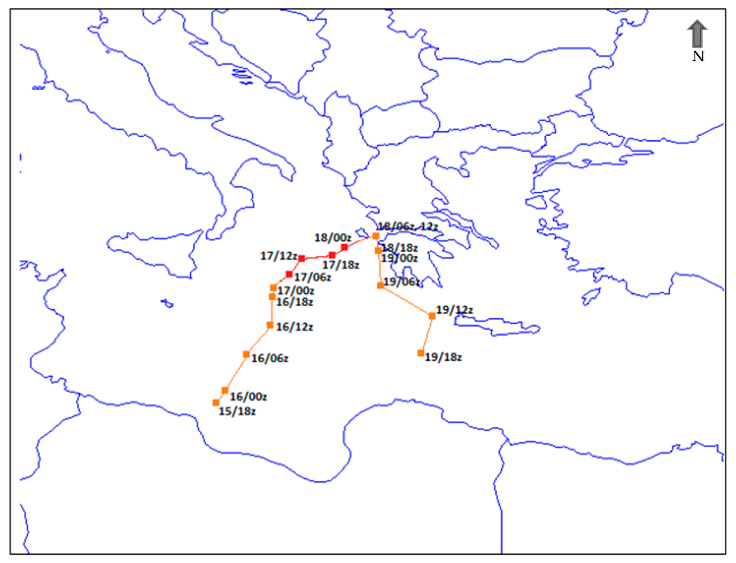
The system under study was formed on 14 September 2020, in the Gulf of Sidra, where the sea surface temperature ranged from 27 to 28 °C. From 15 September, it began to intensify. During 16 September, it traveled a considerable distance (
Figure 1), moving north–northeast. On 17 September, the day it acquired tropical characteristics and was considered a Mediterranean cyclone, it changed its course from north to west toward Greece. Throughout 18 September, it remained trapped in the sea area between Kefalonia, Zakynthos, Aetolia–Acarnania, and Achaia, losing its tropical characteristics but exhibiting the most intense phenomena. Finally, on 19 September, it followed a south–southeast course, reaching southwest of Crete by 18:00 UTC.
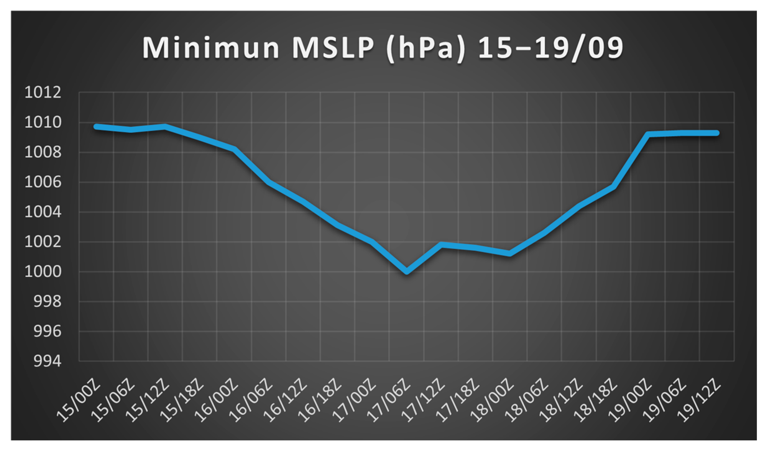
The chart in
Figure 2 shows the minimum central pressure at mean sea level from 15/09 00 UTC to 19/09 18 UTC. Initially, until 16/09 00 UTC, the central pressure decreases at a slow rate. From early morning, it shows a rapid decrease, reaching its lowest minimum value of 999.8 hPa on 17/09 06 UTC at position 37.2° N 18° E. This is also the first time at which it is considered a Mediterranean cyclone with tropical characteristics. From 18/09 06 UTC, the pressure increases rapidly until 19/09 00 UTC, when it starts a steady trend with a value around 1009 hPa.
3. Summary Analysis
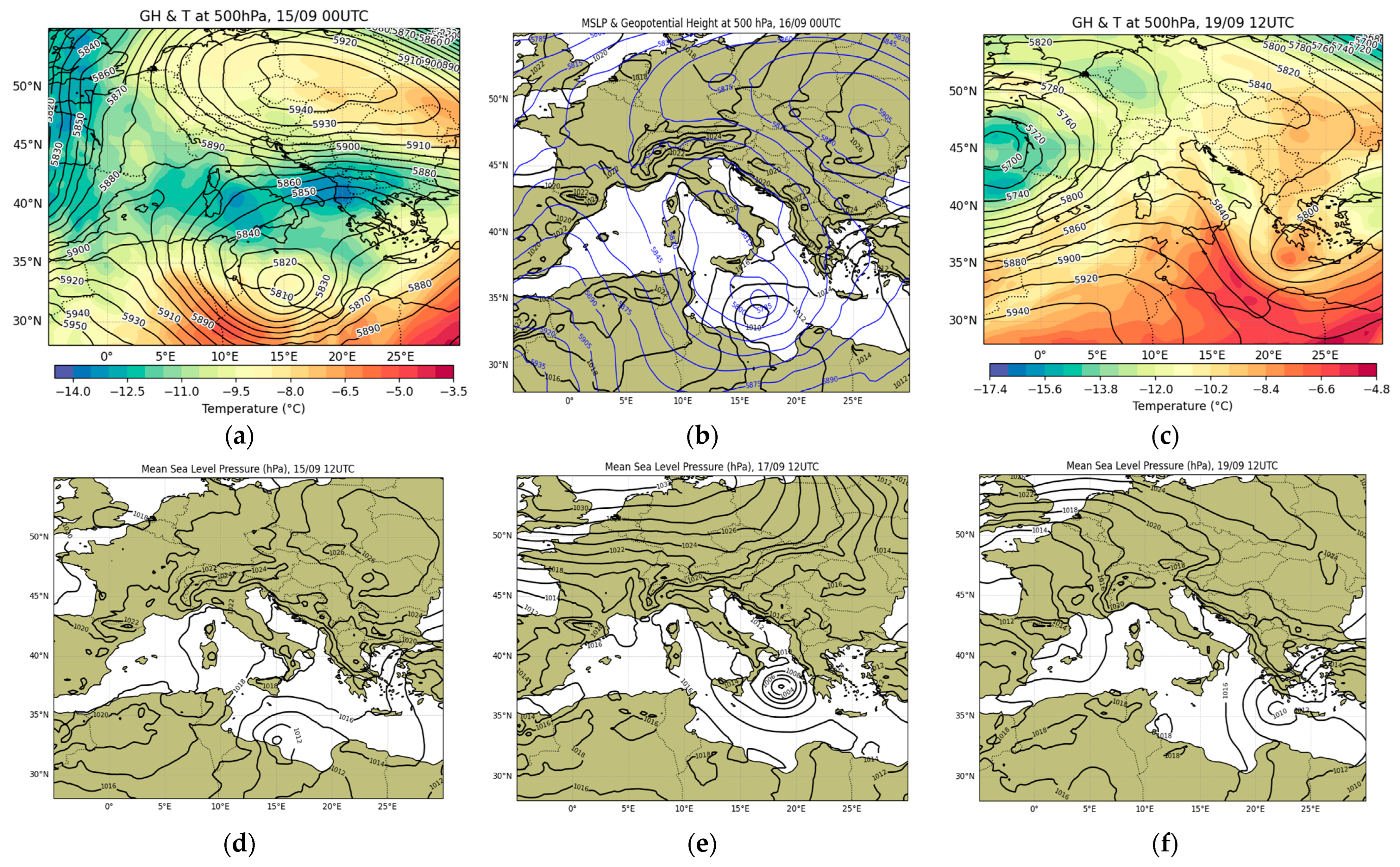
The summary analysis of the upper troposphere on 15 September 2020 is of particular interest as a blocking anticyclone (Rex Block) has established itself over central Europe, while an extensive cut-off low-pressure system is swirling in the Mediterranean (
Figure 3a). This low has isolated colder air masses, creating a cold pool (Dor) in the Balkan-central Mediterranean region with temperatures around −15 °C. This synoptic situation plays a significant role in the initial phase of the phenomenon, as it increases baroclinicity in the lower layers, particularly around the 850 hPa level.
As of 12 UTC on 15 September, the development of the depression had begun without significant changes in atmospheric pressure at the center (~1010 hPa). It remained in the area of the Gulf of Sidra throughout 15 September (
Figure 3d). By 12 UTC on 16 September, it had moved north–northeast and was located at 35.5° N 17.5° E (as well as at 850 hPa, with a geopotential height of 1415 gpm at the center). The pressure at the center continuously decreased, reaching 1005 hPa.
The presence of a cold pool in the middle and upper troposphere, as previously mentioned, is characteristic of an occluded front with a bent-back front structure, as described by the convergence zones (conveyor belts) that characterize a well-formed frontal depression. The center of the low-pressure system at 500 hPa on 16 September at 00 UTC is recorded at 35° N 17° E with 5665 gpm, located west of the surface center (
Figure 3b). The fact that the vertical tilting between the centers of the upper and lower layers is negative (tilting from SE to NW) implies an increase in baroclinicity and an enhancement of the surface pressure drop rate over the next six hours (as observed), based on the quasi-geostrophic approach and the baroclinic model for the development of mid-latitude systems.
On 17 September at 00 UTC, the system had taken the form of a Mediterranean cyclone with tropical characteristics (Mediterranean Tropical Like Cyclone—TLC). The surface low, deepening further to 1002 hPa, was located at 36.7° N 17.5° E (
Figure 4a). One of the notable characteristics at this time is that the center of the system is located at the same geographical area up to the mid-troposphere, indicating the strong barotropic nature of the system, a key feature of TLCs. Therefore, at the 500 hPa isobaric surface, the center is at 36.7° N 17.5° E with a value of 5605 gpm, while simultaneously, the temperature over Greece temporarily rises to −6 °C from −8 °C (
Figure 4a).
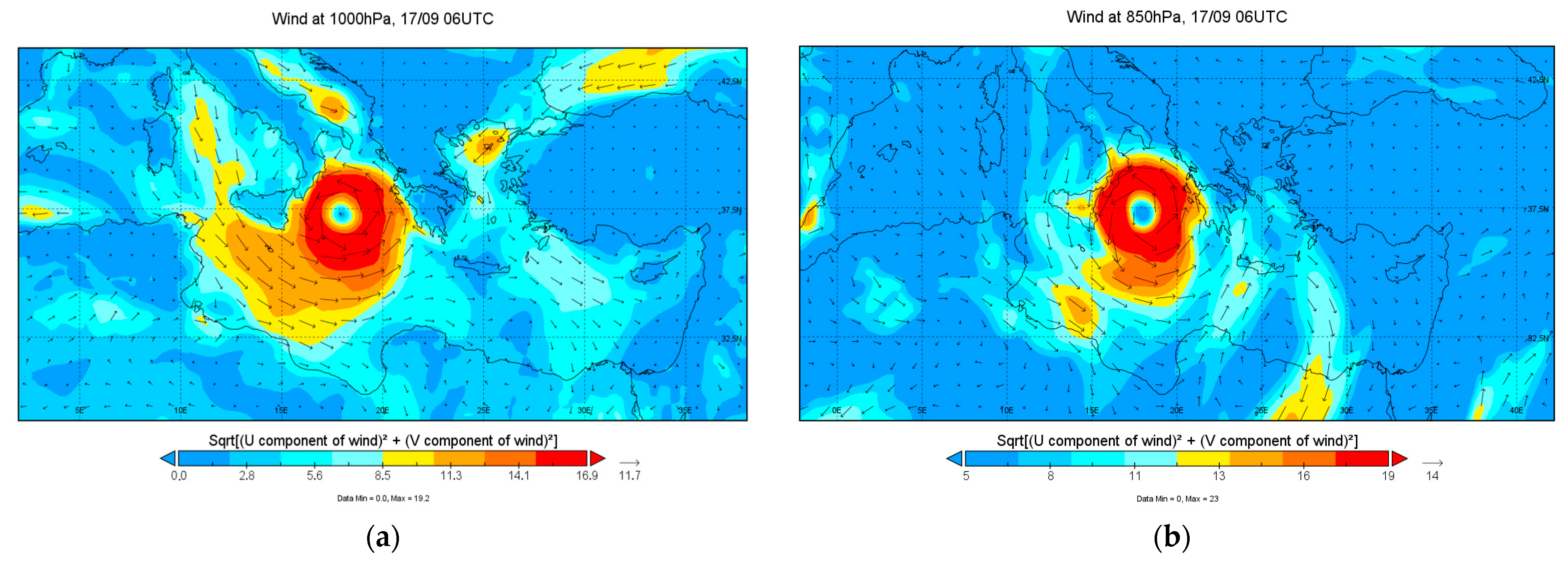
At 06 UTC on 17 September, the system recorded its lowest sea level pressure, reaching 999.9 hPa. Surface winds further intensified, moving cyclonically around the center with speeds reaching 18.5 m/s. Consequently, strong southern winds were initially observed in the central Ionian Sea and subsequently on the islands of Kefalonia, Zakynthos, and Ithaca (
Figure 5a). Symmetry around the center was also evident in the wind field at 850 hPa with a strength of 22 m/s (
Figure 5b). The surface conditions remained largely unchanged six synoptic hours later, at 12 UTC on 17 September (
Figure 3e).
On 18 September at 12 UTC, the phenomena peaked, with heavy rains and thunderstorms occurring until late afternoon in the Ionian, Central Greece, Thessaly, and western Peloponnese. By this time, the center of the surface low remained in the same exact location, but the pressure increased to 1004.4 hPa. At the 850 hPa isobaric surface, the center of the system had a value of 1410 gpm and was located at the same position as the surface low.
At both the 500 hPa and 300 hPa levels, an increase in geopotential heights had begun, indicating the dissipation of the system in the upper layers. Additionally, a branch of the polar jet stream encompassed the disturbance (
Figure 4b,c).
By 12 UTC on 19 September, the surface low continued its southward movement (center at 35.5° N 23° E (
Figure 3f)) without significant changes in sea level pressure. At the 500 hPa level, the convergence trough shifted slightly southeastward, maintaining the NE-SW orientation (
Figure 3c). It no longer exhibited a cyclonic shape, and geopotential heights were rising, with values ranging from 5680 gpm in the east to 5695 gpm in the west over the Greek area. Additionally, a temperature increase of approximately 2 °C was observed.
4. Objective Diagnostic of the Medicane Formation and Evolution
In order to classify a barometric system as a Mediterranean cyclone, a detailed analysis of specific structural characteristics is required. According to [
43], this can be achieved through phase space diagrams, which are based on the B parameter (representing thermal symmetry/asymmetry) and thermal wind. These diagrams enable the assessment of both the frontal nature (lower-tropospheric thickness asymmetry) and the thermal structure (warm or cold core) of a cyclonic system within two layers defined by equal pressure intervals.
This evaluation is carried out using the B parameters (thermal symmetry/asymmetry) and the thermal wind, respectively. Specifically, the B parameter is calculated as the difference between the mean geopotential thicknesses on the right and left sides of the low, relative to its motion, at each time step and for two isobaric layers: the upper layer (600–300 hPa, B
U) and the lower layer (900–600 hPa, B
L). In addition, the thermal wind is computed within these layers, namely V
TL and V
TU. Although a 500 km radius was used in the study of tropical cyclones by [
43], a 200 km radius was considered more appropriate in this work, given that Mediterranean tropical-like cyclones are smaller in scale, and using a larger radius could potentially smooth out their distinguishing features [
44,
45].
The scaled thermal wind magnitude parameters are defined as follows:
where Δ
Z is the difference between a maximum and minimum value of geopotential height at the specific isobaric level within the employed circle with a radius of 200 km around the minimum MSLP of the low every 6 h.
In order to avoid extrapolation into sub-surface levels or within the atmospheric boundary layer, pressure levels below 900 hPa were excluded from the calculation of the relevant parameters. Similarly, levels above 300 hPa were omitted to eliminate potential interference from stratospheric influences, which often exhibit behavior contrary to that of the troposphere. Consequently, the analysis of cyclone characteristics focuses on the 900–600 hPa range for the lower troposphere and the 600–300 hPa range for the upper troposphere, consistent with methodologies adopted in earlier research [
5,
43,
44,
46].
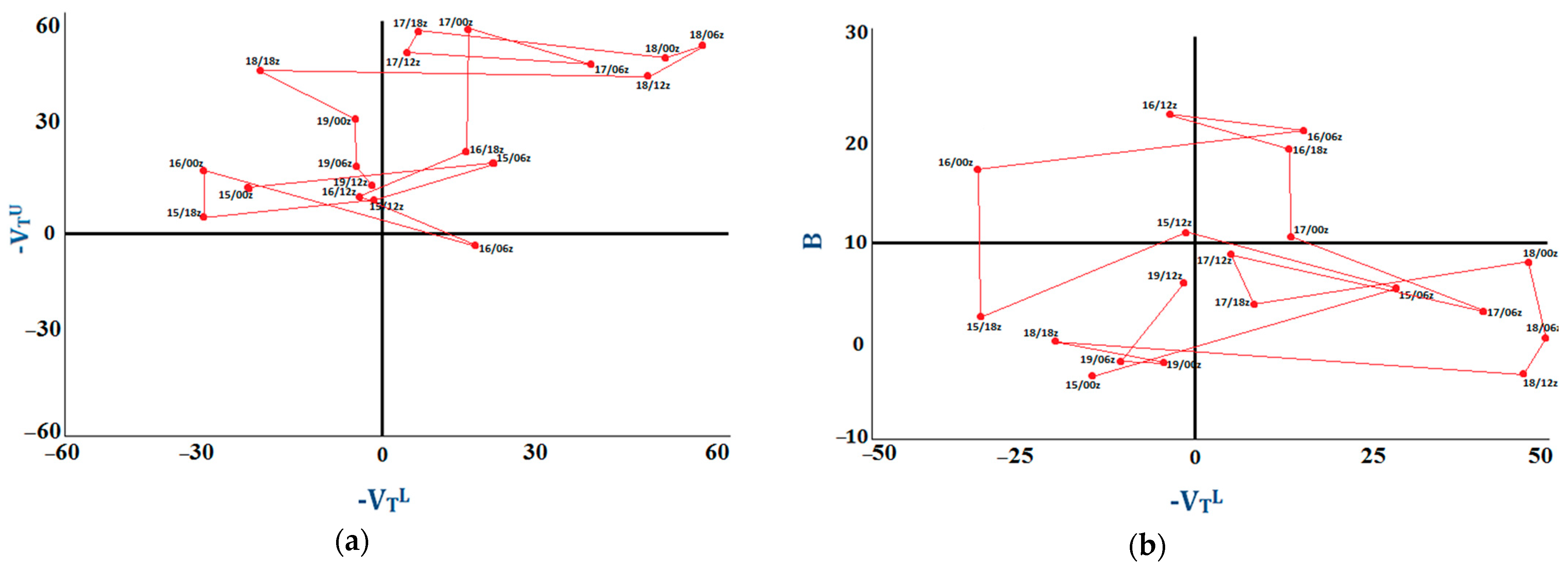
Low values of the B parameter (B < 10 m) indicate a thermally symmetric system, similar to tropical cyclones. The thermal wind determines whether the system has a warm or cold core. When the values of −VTL and −VTU are positive (−VTL > 0, −VTU > 0), the core is considered warm. Therefore, for a cyclone—whether tropical or a Mediterranean medicane—to be classified as warm-core and symmetric, the following criteria must be met: B < 10 m, −VTL > 0, and −VTU > 0.
According to
Figure 6, which presents the B parameter, −V
TL, and −V
TU every 6 h, the system’s warm-core structure began to form at 18 UTC on 16 September. However, by 00 UTC on 17 September, it had not yet developed a symmetric structure. The deep, symmetric warm-core structure observed throughout the troposphere from 06 UTC on 17 September to 12 UTC on 18 September indicates the transition to a tropical-like Mediterranean cyclone (medicane). From 18 UTC on 18 September, the cyclone’s core became cold at lower levels while remaining warm at upper levels, maintaining its symmetric structure. After 12 UTC on 19 September, the system no longer exhibited the structure of a medicane and attained characteristics of an extratropical cyclone.
5. Dynamic Study
5.1. First Phase
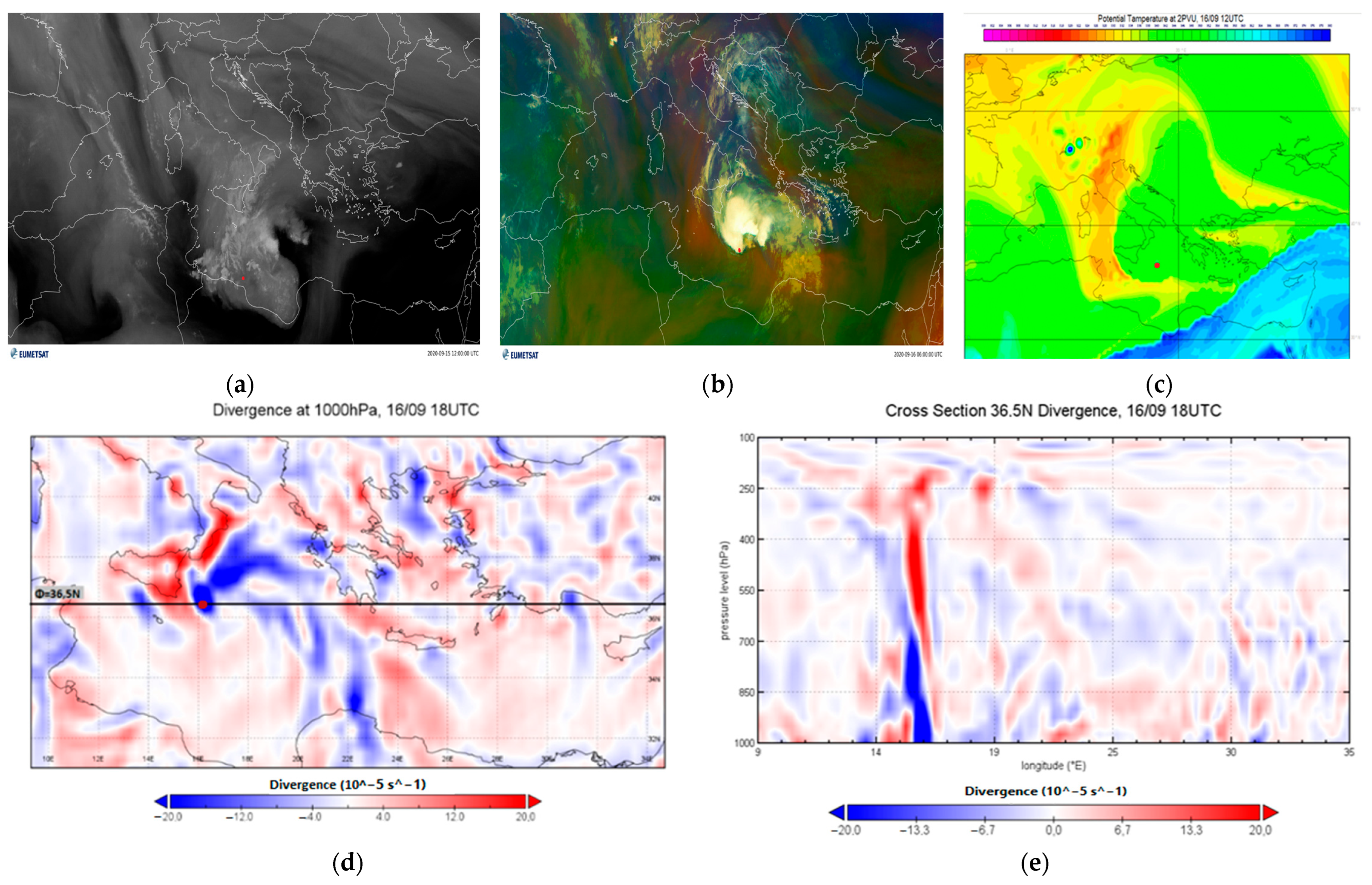
At 12 UTC on 15 September, the satellite image in the water vapor channel (
Figure 7a) showed the presence of an extensive cloud layer over the area of Northern coastal Libya and Southern Italy, which resembles the characteristics of a baroclinic leaf. This is also reflected in the corresponding infrared spectrum image (
Figure 7b) and marks the beginning of the creation of a baroclinic zone in the lower layers of the troposphere. It also indicates the possible onset of surface frontogenesis to the east of a barometric trough in the upper layers [
47], suggesting the presence of a PV anomaly along it, characterizing the area with significant moisture or substantial cloud cover. A critical aspect of the upper-level dynamics is the appearance of a moisture gradient (or high PV values) south and west of the baroclinic leaf (intense dark area), as depicted in the satellite image in the water vapor channel at this time. This indicates the presence of an upper-level jet streak in this region.
At 06 UTC on 16 September, based on the satellite image of the Airmass index, a branch of the jet stream is located south of the disturbance (yellowish colors in
Figure 7b), feeding it with dry and cold air masses. Additionally, the blue and green colors in the broader Mediterranean region indicate air masses with different thermo-hygrometric characteristics and, consequently, the formation of frontal surfaces.
The analysis of dynamic temperature distribution on constant potential vorticity surfaces helps in identifying baroclinic zones and the jet stream, as well as the maxima or minima of dynamic temperature over an area, which are referred to as cold or warm anomalies, respectively [
48,
49]. The distribution of dynamic temperature at the 2 PVU surface for 12 UTC on 16 September (
Figure 7c) shows a cold anomaly in a zone west of the examined depression. This indicates that stratospheric air has descended into the upper troposphere and constitutes a stratospheric intrusion or tropopause folding, according to Hoskins et al. [
49].
The cross-section shows the vertical distribution of divergence from the 1000 hPa level up to the 100 hPa level (
Figure 7e). The divergence is multiplied by 10
5, so its unit of measurement is 10
−5 s
−1. Positive values indicate divergence, while negative values indicate convergence. Throughout 16 September, convergence was intense in the system’s area (
Figure 7d), with the zero divergence point continuously located at a lower altitude (approximately 3000 m). At 18 UTC, the zero divergence point is found at the 700 hPa isobaric surface, along the 16° E meridian. For the system, this day is a development day on which the upward motion at the surface was triggered primarily by the low-level convergence.
5.2. Second Phase
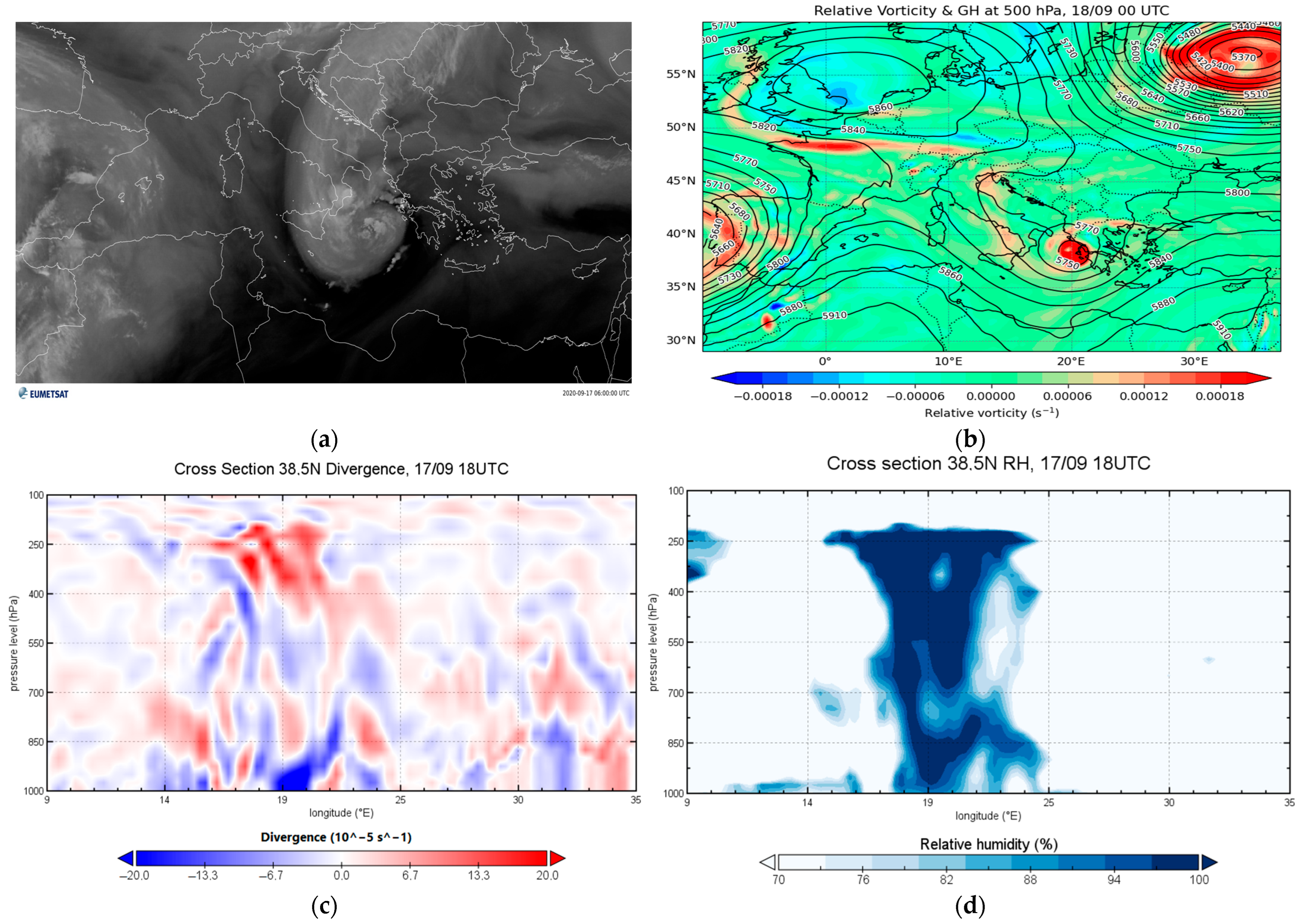
At 06 UTC on 17 September, the system had taken the form of a Mediterranean cyclone with tropical characteristics (from 03 UTC). The cyclonic disturbance continued to be accompanied by a branch of the jet stream associated with stratospheric air intrusion into the mid-troposphere, as confirmed by the MSG satellite image in the water vapor channel 6.2 μm (
Figure 8a).
In this situation, it is useful to examine the distribution of divergence and relative humidity at latitude 38.5° N. It is evident that at 18 UTC on 17 September (
Figure 8c,d), the trend in the distribution of divergence remains unchanged compared to previous observations (
Figure 7d,e). Convergence persists at the surface and lower levels, while divergence is present at upper levels. Meanwhile, relative humidity is greater than 100% with a vertical zone from the 950 hPa level up to 210 hPa, indicating an over-saturated atmosphere. All of this occurs between longitudes 18.5° E and 20° E, which is quite close to the cyclone’s center.
At 00 UTC on 18 September, at the 500 hPa level, as the center of the TLC approaches the islands of the central Ionian Sea, positive vorticity is observed with the maximum value at the center, i.e., at 37.7° N 20° E (
Figure 8b). The corresponding surface low is also recorded at the exact same position, indicating that the system is characterized by zero vertical tilt (barotropic).
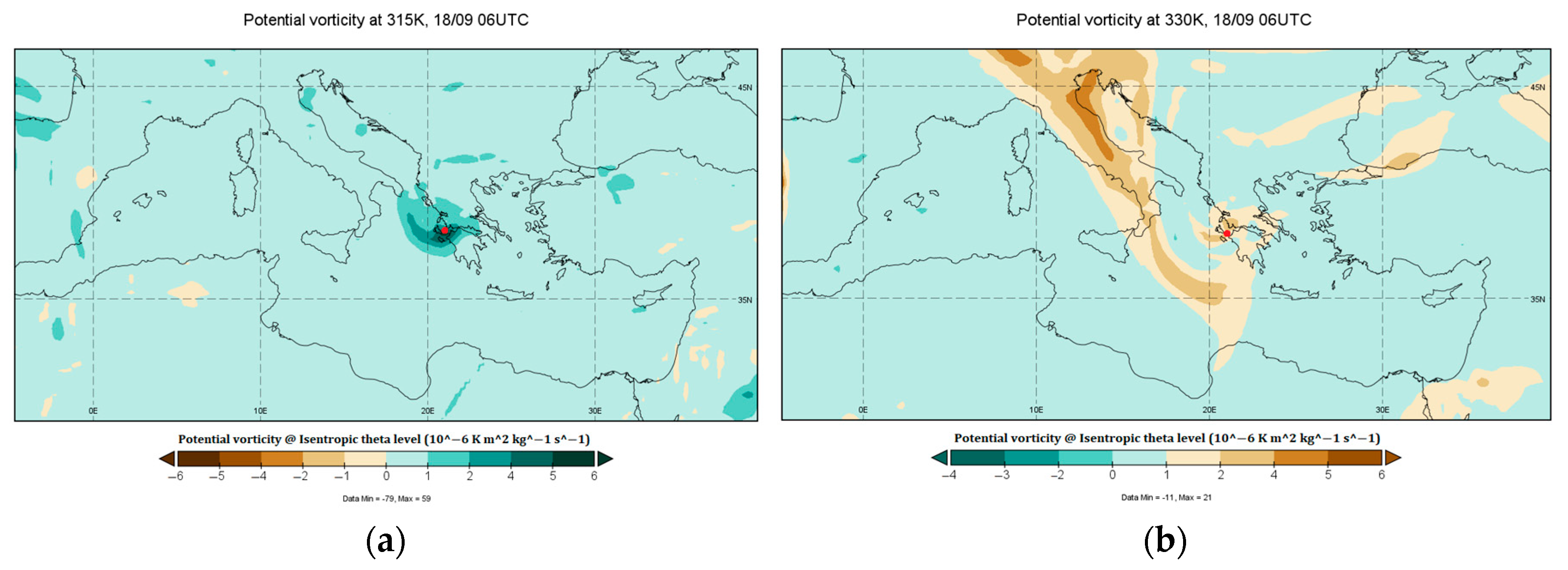
Analysis of the 315 K and 330 K isentropic surfaces (
Figure 9)—which approximately represent the tropopause—revealed potential vorticity values exceeding 2 PVU to the west and south of the cyclone at 06 UTC on 18/09. These findings indicate the presence of a tropo-pause fold, which peaked shortly after that time.
5.3. Third Phase
From midday on 18 September, the system loses its tropical characteristics and evolves into a strong extratropical barometric low, swirling with its center over the sea area between Kefalonia, Zakynthos, and Achaea.
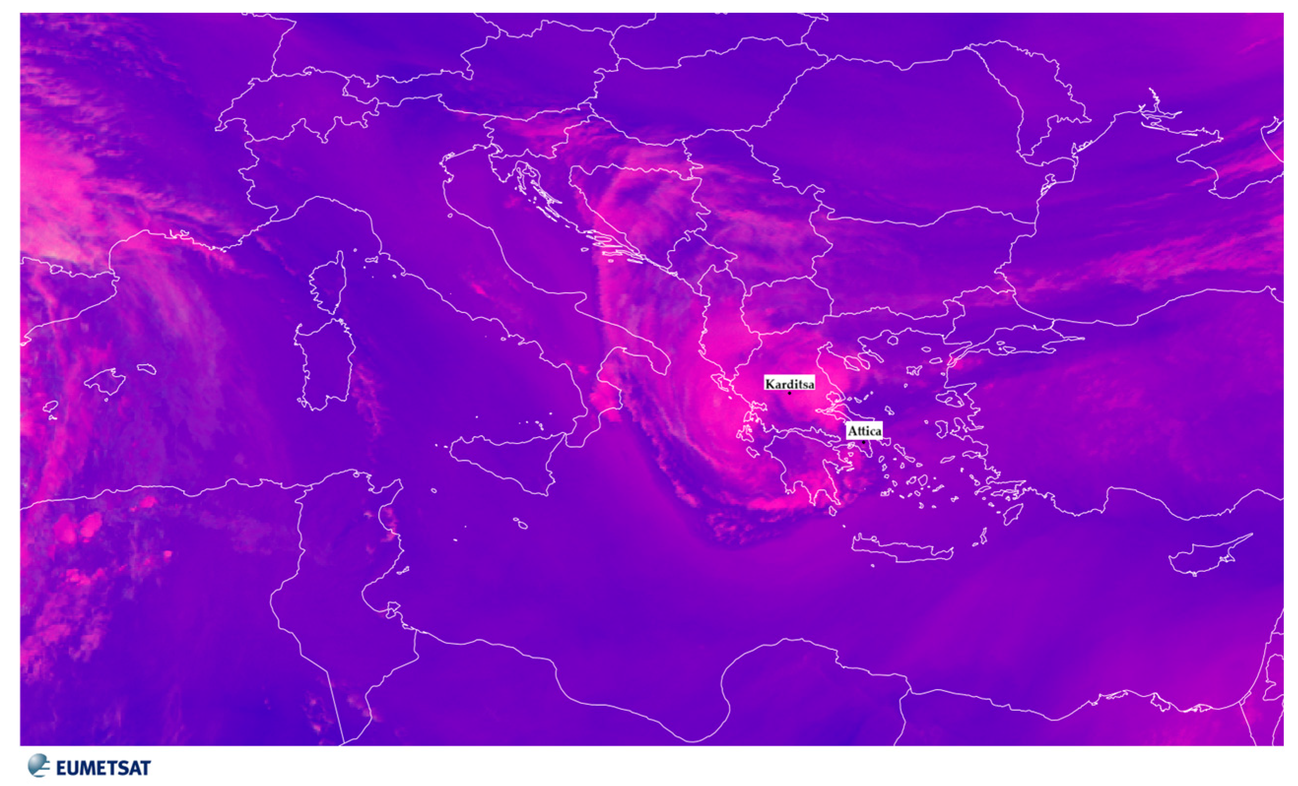
Shortly after 12 UTC on 18 September, the vertical development of cumulonimbus clouds began in the Thessaly region (
Figure 10). This phenomenon was triggered by the intensification of southeasterly to northeasterly winds, which created convergence in the broader Karditsa area, resulting in strong rainfall and thunderstorms.
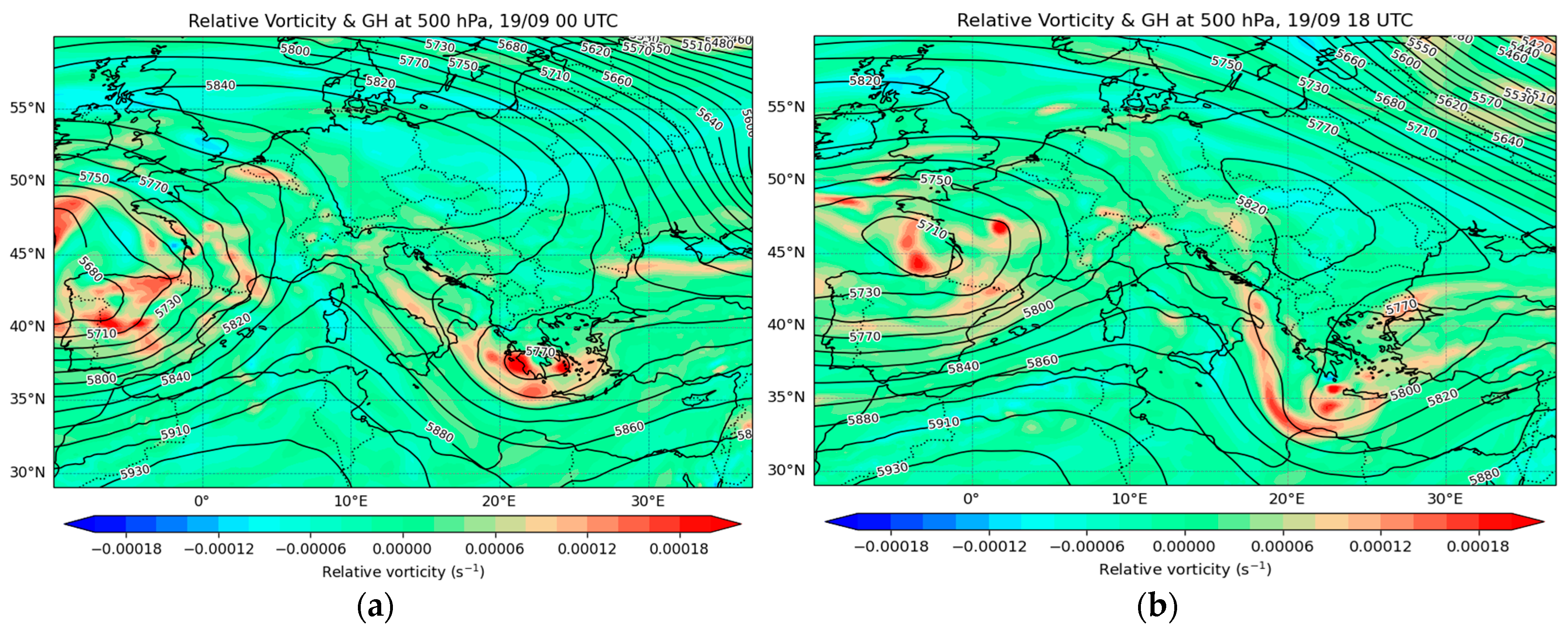
At 00 UTC on 19 September, relative vorticity was detected over the Greek region at the 500 hPa isobaric surface (
Figure 11a), with maximum values again over the surface low located at 37.7° N 21.2° E. Significant values were also observed in the sea area east of Attica, where some phenomena are occurring. However, these values were lower as the system had transitioned from the strengthening phase to the weakening phase.
By 18 UTC on 19 September, the values of relative vorticity at the 500 hPa isobaric surface had decreased significantly (
Figure 11b), indicating a weakening of the dynamics in the upper layers and further degeneration of the surface low. Despite this, rainfall persisted between the Peloponnese and Crete.
6. Dynamics of Lower Strata
It has now been proven that the formation and development of Mediterranean cyclones are favored by marginally positive anomalies in Sea Surface Temperature [
30]. The study of surface fluxes also includes a detailed examination of sea surface temperature.
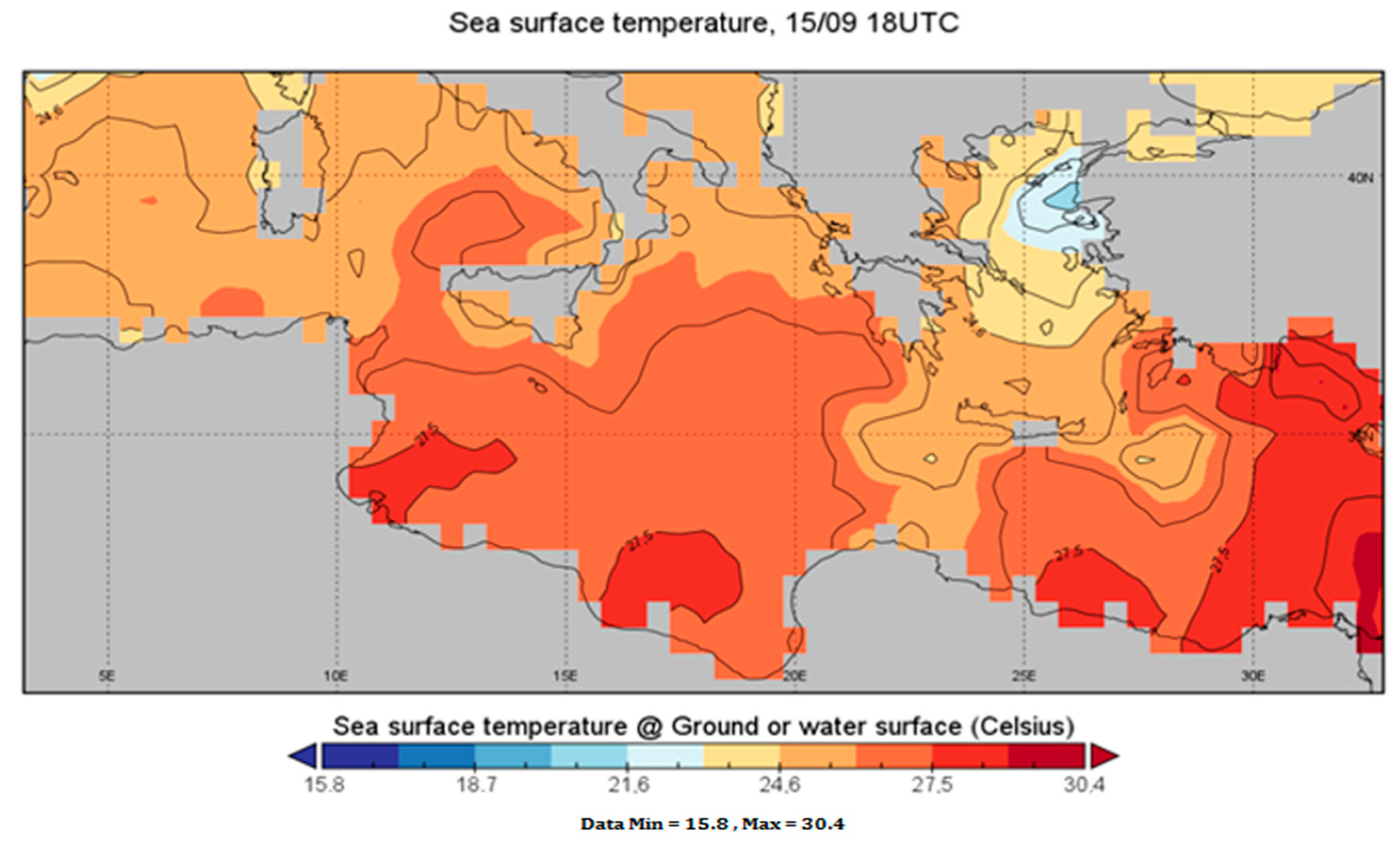
As early as 15/09, the surface temperature in the area of the Gulf of Sirte was notably high. At 18:00 UTC on 15/09 (
Figure 12), the temperature variation from the coasts of Libya to the coasts of western Greece was significant, around 4 °C, with areas in the Gulf of Sirte reaching between 27.5 °C and 28 °C.
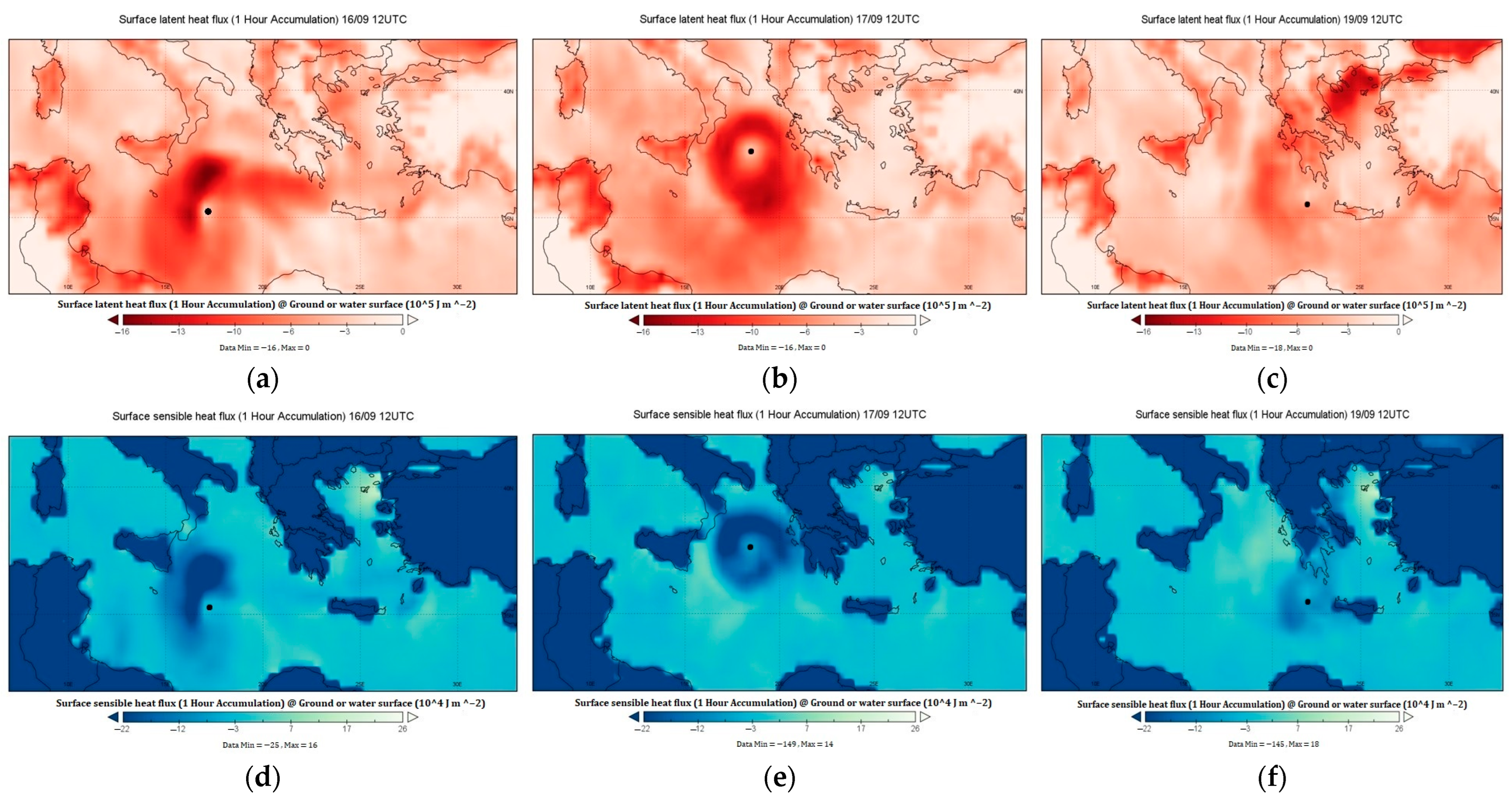
The absolute values of the heat fluxes are particularly high in the region in which the phenomenon develops. Negative latent and sensible heat flux values indicate fluxes from the surface to the atmosphere, promoting the convection process. On 16/09, the negative surface heat fluxes intensified in the western and northwestern parts of the depression (
Figure 13a,d), areas where, during the morning of 16 September, the maximum wind intensity—with a clearly northwesterly direction—was observed. This behavior is typical, as both types of surface heat fluxes are linearly dependent on wind intensity [
50].
Throughout 17 September, negative heat fluxes—both latent and sensible—were observed, uniformly distributed around the system’s center (
Figure 13b,e), gradually weakening in magnitude until the system reached its minimum atmospheric pressure.
On 17/09 at 18 UTC, when the surface heat fluxes were at their strongest, surface winds reached 8–9 Beaufort, primarily in the southern Ionian Sea, where the maximum wave height of 9 m was also recorded. In general, very high waves, ranging from 6 to 7 m, dominated the rest of the Ionian Sea.
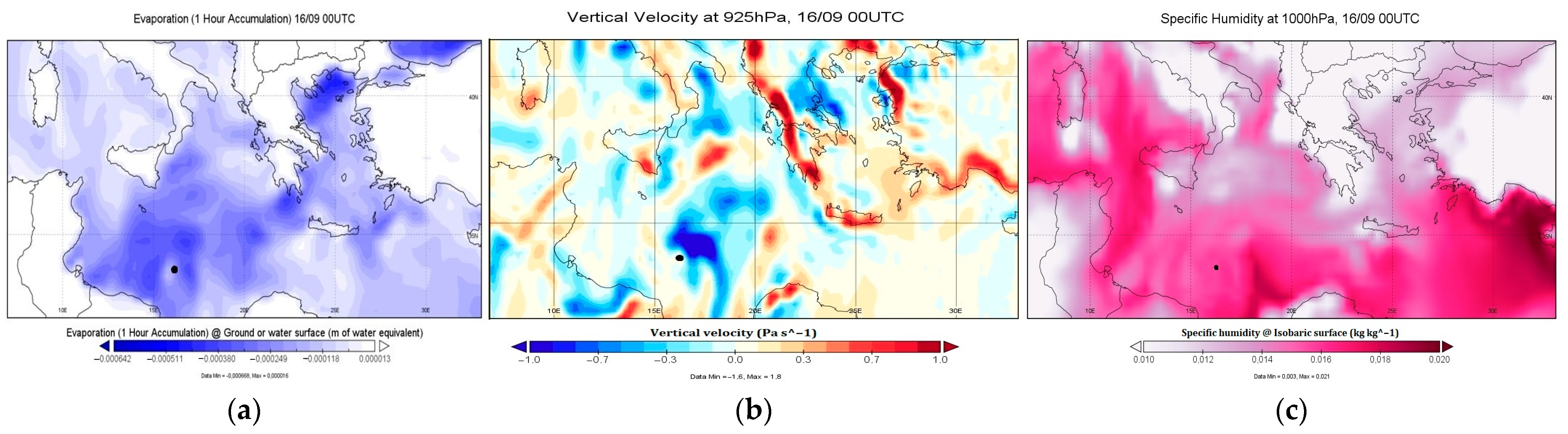
The increased evaporation in the area, from the coasts of Libya to the coasts of Sicily, combined with the upward movements prevailing in the lower atmosphere, is indicative of diabatic processes at the level of the barometric low (
Figure 14a). In terms of vertical atmospheric motions, negative values of the ω component of the wind indicate upward movements, measured in Pa/s. Simultaneously, the maxima of these upward motions in the lower atmosphere are located in the same region of increased evaporation (
Figure 14b), further highlighting the role of diabatic processes in the development and evolution of the depression. Evaporation involves the absorption of latent heat, which is released when water vapor condenses as the air mass is forced to rise into higher atmospheric layers.
Due to evaporation, specific humidity at the sea surface increased during the early stages of the depression. The highest values, observed on both 15th and 16th September, were concentrated in the Gulf of Sirte, which also corresponded to areas with the highest surface temperatures. A sharp increase in specific humidity was noted at 00 UTC on 16/09 (
Figure 14c), approximately 30 h before the minimum atmospheric pressure at mean sea level was recorded. This suggests that the moisture in the lower layers was “absorbed” by the air masses as the depression passed over the warm sea surface. This process led to the condensation of water vapor, releasing latent heat. Hence, the condensation of water vapor preceded the deepening of the system. This observation indicates that the higher sea surface temperatures were a key factor in the explosive deepening of the depression.
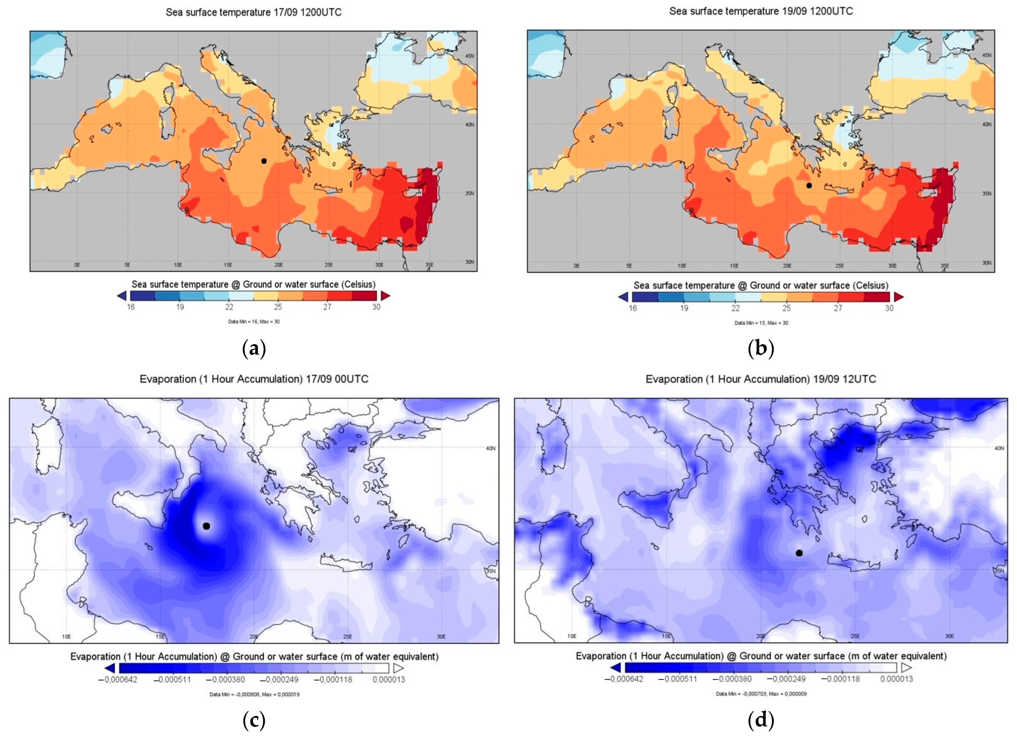
By 12 UTC on 19/09, as the system had significantly weakened and was slowly moving south (positioned west of Crete as shown by the black dot), the enhanced negative heat fluxes showed a marked weakening. This was due to reduced temperature differences affecting the transfer of sensible heat. Due to sea surface cooling from intense evaporation (
Figure 15a,b), the flow of sensible heat also decreased. This was caused by the significant reduction in temperature differences (
Figure 16). Additionally, as the system made landfall (in the Peloponnese), its moisture and energy supply were cut off, while frictional forces increased. As a result, latent heat values declined.
The changes in heat fluxes are also reflected in the evaporation patterns. High evaporation rates were observed at 00 UTC on 17/09 (
Figure 15c), from the southern coasts of Italy to the central Ionian Sea, coinciding with the area covered by the Mediterranean cyclone. By 12 UTC on 19/09 (
Figure 15d), a significant decrease in sea surface evaporation was observed. This decline is attributed to the re-evaporation of precipitation, which progressively diminished the subsaturation of the cyclone’s circulation, thereby reducing the efficiency of surface evaporation. Additionally, the reduction in evaporation is linked to changes in wind intensity, as evaporation is strongly associated with wind gradients.
7. Conclusions
This study examined the genesis, evolution, and dynamic and thermodynamic characteristics of a depression in the central Mediterranean from 15 to 19 September, which exhibited Mediterranean cyclone characteristics with tropical features for approximately 30 h. Data for various meteorological variables were sourced from the new and improved ERA5-Interim time series of ECMWF reanalysis products, on a regular 0.25° × 0.25° latitude–longitude grid.
A three-phase framework was adopted to analyze the cyclone’s evolution, initially defined through Hart phase diagrams and subsequently confirmed through dynamic analysis. During the first phase (15 September), the structures of the upper troposphere began to strengthen, contributing to the reconstruction of the parent barometric low in the Gulf of Sirte, which had been present since 13 September. This strengthening was mainly due to dynamic processes in the upper layers of the atmosphere. During this phase, the system began moving northeastward, heading toward Greece. In the second phase, during which the Mediterranean cyclone formed, diabatic processes at the lower levels, such as latent heat, dominated, without significant support from baroclinic processes in the upper troposphere. In this phase, the system is characterized as barotropic, as it evolved independently of the upper layers, and it was the phase when the system approached the western regions of Greece, bringing heavy rains, thunderstorms, and gale-force winds. Finally, in the third phase, the system maintained its barotropic character (as it began moving southward), but it showed a continuous weakening tendency, reflected in the gradual increase in sea surface pressure. This three-phase evolution highlights the complex interaction between dynamic and thermodynamic processes in the life cycle of Mediterranean cyclones with tropical characteristics.
The general atmospheric setup during this period was characterized by an anticyclone over central Europe and a detached low in the central Mediterranean (Rex Block). From its initial phase, the system displayed baroclinic wave characteristics, as indicated by the strong baroclinicity aloft, evident in the westward tilt of the low centers (negative slope from the surface to the upper troposphere). This baroclinic structure contributed to increasing the system’s available potential energy during its intensification.
In the Gulf of Sirte, sea surface temperatures were notably high (SST~28 °C), creating significant thermal gradients that promoted baroclinicity in the lower layers. Simultaneously, the transport of cold air masses in the upper troposphere over the central Mediterranean facilitated cyclogenesis. Surface heat fluxes played a critical role in the system’s development, with increased wind speeds intensifying these fluxes.
The central pressure of the low began to decrease on the afternoon of 15 September, reaching its lowest at 06 UTC on 17/09 (999 hPa). By 00 UTC on 17/09, the centers of the system had vertically aligned across all isobaric surfaces (no vertical tilt), indicating that the system had entered its most efficient phase.
The divergence in the upper troposphere over the system’s center was crucial throughout its intensification phase, especially when it was classified as a Mediterranean cyclone. Based on divergence distribution, the maximum divergence was located directly above the system’s center.
As the system moved northward, acquiring tropical cyclone characteristics, warmer air at its center became encircled by cooler air in the mid and upper troposphere, creating a well-defined warm core. A compressed front with spiraling cloud bands also developed around the system.
Moreover, a tropopause fold was observed in the study area, peaking shortly after 06 UTC on 18/09. This was evidenced by high potential vorticity values (pv ≥ 2 PVU) on the 315 K and 330 K isentropic surfaces, low potential temperatures on the pv = 2 PVU isentropic surface, and airmass satellite imagery. These factors, in line with the theory of dynamic vorticity by Hoskins et al. [
49], favored the development of updrafts east of the upper troposphere downdraft zone.


