Development of Surface Data Assimilation Using Simplified Extended Kalman Filter in AROME Model in Hungary

Abstract

Accurately representing land–atmosphere interactions is essential for numerical weather prediction models, as they have a significant effect on forecasted near-surface meteorological parameters. We used the SURFEX soil model, coupled with the AROME non-hydrostatic numerical weather prediction model at HungaroMet Hungarian Meteorological Service. Land data assimilation techniques are employed to provide the most accurate initial conditions for the AROME-SURFEX system. Initially, the Optimal Interpolation (OI) method was applied to determine the initial conditions for soil temperature and moisture. This study focuses on implementing the more complex and advanced Simplified Extended Kalman Filter (SEKF) for surface data assimilation. The SEKF corrects the soil temperature and soil moisture content using screen-level observations (2-m temperature and relative humidity), offering improvements over OI. We highlight the advantages of the SEKF across different seasons, noting that it is a more physically-based approach with dynamically varying Jacobians. We demonstrate how outlier Jacobians can be filtered using linearity check to handle system nonlinearity. The tuning of appropriate data assimilation parameters, such as observational and background errors, is also crucial for achieving optimal results. We evaluate the impact of the SEKF by conducting forecast verification against in situ atmospheric observations, comparing its performance with that of OI. Our results indicate a significant improvement in winter forecasts. Additionally, a moderate improvement is observed in spring, highlighting the seasonal dependency of the efficiency of the SEKF.

1. Introduction

For the accurate forecasting of meteorological conditions in the near-surface atmospheric layers, it is crucial to describe the surface–atmosphere interaction as comprehensively and precisely as possible. Based on the reliability of the observations and the previous model forecast (background or first guess), they are combined in a statistically optimal way using data assimilation (DA) techniques in numerical weather prediction models (NWP). Recently, several types of algorithms have been widely used, including optimal interpolation (OI) [1,2,3], which minimizes the expected mean squared error between analysis and the truth; variational methods, which are based on the minimization of the cost function that measures the misfit between the analysis and the background and between the analysis and the observations [4]; and the Kalman Filter, which captures the flow dependence of the background error covariance. Land surface assimilation most commonly uses OI [1], although the extended Kalman Filter (EKF) and the Simplified Extended Kalman Filter (SEKF) versions are becoming increasingly popular [5,6].

In ALADIN (Aire Limitée Adaptation dynamique Développement InterNational), which was one of the earliest NWP models run in Hungary, the initial conditions for the soil were interpolated from the analysis fields of the ARPEGE (Action de Recherche Petite Echelle Grande Echelle) global model. Since 2008, we have used CANARI (Code for the Analysis Necessary for Arpege for its Rejects and its Initiation) optimal interpolation [7,8], which determines soil temperature and moisture analysis based on the relationship between soil and near-surface variables.

The AROME (Application of Research to Operations at Mesoscale) model consists of the non-hydrostatic dynamic core of ALADIN, the atmospheric physical parameterization of the Meso-NH research model, and the SURFEX (SURface EXternalized) surface model [9]. Initially, the surface analysis from the 10 km resolution ALADIN model was interpolated onto the 2.5 km resolution grid of AROME, and then since 2016 the improved version of OI has been directly used on the AROME grid [10,11]. The surface assimilation based on OI consists of the quality control of the observations, the analysis of the 2-m temperature and relative humidity, and the corresponding correction of the surface and soil parameters (temperature and water content) [2]. At the same time, experiments began with the SEKF, opening the door to the use of new monitoring techniques—such as remote sensing data.

The SEKF enables the assimilation of conventional (measured at 2 m) and non-conventional (e.g., satellite) observations. The advantages of the assimilation of MetOp ASCAT soil moisture and SPOT/VGT leaf area index (LAI) satellite data were verified by running only the soil model for a long period, regardless of the atmospheric model [12,13,14]. In their experiments, the SURFEX model was run with prognostic vegetation, allowing the state of the vegetation to adapt to changing environmental conditions. The model is able to describe photosynthesis and plant death. It has been shown that the results can be further improved by assimilating the LAI (available every 10 days) and soil moisture (daily) measurements, the variability of the vegetation within the year, and the beginning and length of the growing season, and the maximum of the biomass within the year can also be further specified. By using a multi-layer soil scheme [15], the description of heat and moisture transport between the 14 soil layers is also more accurate and detailed. Ref. [16] showed that the upper 60 cm layer of the soil is sensitive to the assimilation of soil moisture, and below that no effect can really be detected. The description of aboveground biomass, evapotranspiration, and the carbon cycle is significantly improved, and extreme events such as droughts can be well monitored even on a global scale.

In addition to the above, the SEKF can also be used in the surface data assimilation of operational forecasting models. It has been used in the ECMWF (European Centre for Medium-Range Weather Forecasts) since 2010 in the global operative (Integrated Forecasting System—IFS) model. Initially, only the 2-m temperature and relative humidity were assimilated with the SEKF [5], then the MetOp-B and MetOp-C satellites ASCAT and soil moisture measurements made with the SMOS neural network were also included in the assimilation cycle [17]. Since 2019, the Jacobian members of the SEKF have been produced by the ensemble spread of the 2-m variables and soil moisture, thereby enhancing the description of the relationship between the atmosphere and the land [18].

The Met Office also uses the SEKF in its global model surface data assimilation system, using screen-level temperature and relative humidity and ASCAT soil moisture measurements [19]. For the global model experiments, results were presented separately for the Northern and Southern Hemispheres. In winter, in the Southern Hemisphere, the ASCAT assimilation has led to an approximately 2% improvement in the temperature forecast. Whereas in the Northern Hemisphere in summer, using ASCAT data, approximately 1% deterioration was observed, but this could also be improved by including the 2-m observations into the surface data assimilation. In contrast, in the Southern Hemisphere, the positive impact came from the incorporation of ASCAT soil moisture observations. In addition, there has been a significant improvement in hydrological forecasting across the United Kingdom.

The Australian Bureau of Meteorology, in collaboration with the Met Office, also operationally applies the SEKF to 2-m variables and ASCAT and SMOS satellite soil moisture surface data assimilation in the ACCESS model [20]. When the Jacobians were investigated, they found a strong relationship between the temperature at 2-m observations and the moisture in the upper layer of the soil. During the day, the sign is negative, while at night it is positive. The connection between the relative humidity of the 2-m observations and the moisture of the deeper soil layers is determined by the transpiration of the plants, which is stronger during daylight hours and also depends on the thickness of the root zone. While the link between the 2-m parameters and soil temperature is high near the soil surface, it rapidly decreases further down.

The Indian National Center for Medium-Range Prediction found that ASCAT soil moisture assimilation significantly improved the analysis and prediction of tropical cyclones [21]. The prediction of the position and strength of the cyclone was also improved by using ASCAT data, the amount of precipitation and the location of maxima, and even the stability indices became more accurate.

This study demonstrates the advantage of using the Kalman Filter method for surface data assimilation, compared to the OI in the operational environment at the HungaroMet (Hungarian Meteorological Service). The assimilation of screen-level observations (2-m temperature and relative humidity) indicates the correction of the soil temperature and moisture content by the SEKF in AROME. In Section 2, the AROME model and the used surface data assimilation methods are described. In Section 3, we present the results, with a special focus on the evaluation of the Jacobians, how to correct the nonlinearity in the system, the study of the analyses increments, and the verification of model forecasts. Finally, a summary of the recent results and further potential research are provided.

2. Materials and Methods

The land surface analysis is performed independently and in parallel with the atmospheric 3D-Var analysis, because the two systems operate on different physical principles and time scales and require different types of observations. Performing them separately ensures optimal assimilation of surface and atmospheric data. These two analyses then provide the initial conditions for the short-range forecast of the AROME-SURFEX system. In this section, the AROME numerical weather prediction model and the coupled land model, SURFEX, are presented (Section 2.1).

In this study, two land data assimilation methods are applied: OI-MAIN and the SEKF. OI-MAIN (Optimal Interpolation for MAIN Initialization) is a relatively simple and computationally efficient technique based on Optimal Interpolation. The SEKF, on the other hand, is a more advanced method that takes into account the nonlinearities in the observation operator and uses local sensitivities of the model, offering improved performance in certain situations. These methods are discussed in more detail in Section 2.2 and Section 2.3, respectively.

2.1. AROME Model

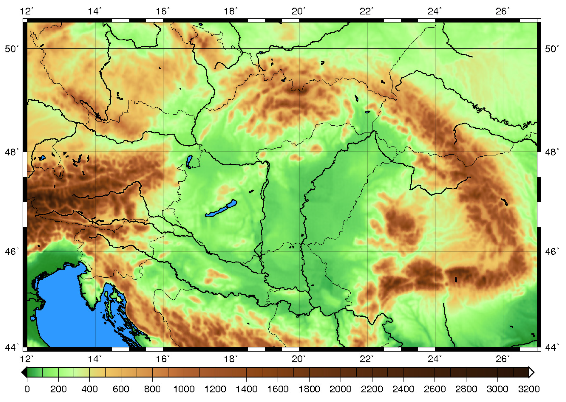
The AROME cy43t2 non-hydrostatic forecast model was run at HungaroMet eight times a day (at 0, 3, 6, 9, 12, 15, 18, and 21 UTC), 48 h ahead. The domain covers the Carpathian Region with a horizontal resolution of 2.5 km and a vertical resolution of 60 level (Figure 1). In the upper air, 3D-Var is used with a 3-hourly cycle and a 3-hourly assimilation window [10,11]. We assimilate measurements from synoptic stations (2-m temperature and relative humidity, 10-m wind, and station level pressure), radiosondes (temperature, humidity, wind, and geopotential height), AMDAR and Mode-S MRAR aircraft observations (wind, temperature, and humidity), and GNSS-ZTD data. The soil model of the AROME is the SURFEX 8.0 model [22], which can be used directly coupled (online) to the atmospheric model as well as independently in offline mode. SURFEX describes the transport of heat and moisture between the atmosphere and the soil, and between different layers of the soil.

In the SURFEX system, each surface grid point is separated into 4 different tiles: nature, sea, lake, and urban. The model handles each tile independently, solves the prognostic equations for soil moisture and temperature and calculates the surface fluxes separately for the different tiles.

The nature tile is simulated with the ISBA (Interaction Soil-Biosphere-Atmosphere) scheme, which computes the exchanges of energy and water between the continuum soil–vegetation–snow and the atmosphere above [23,24]. In ISBA, a 3-layer soil scheme is used (surface 0–1 cm, root zone 0–2 m, and deep soil 2–3 m). The soil prognostic variables (temperature and water content) are calculated using the force–restore method. The force terms represent the external forcing on the system, e.g., radiative fluxes, precipitation, and latent and sensible heat flux. The restore term describes how the system reaches equilibrium and relaxes the soil to return to the mean temperature or water content.

Surface parameters are defined by physiographic databases: GMTED2010 for orography [25], ECOCLIMAP-II for surface covers [26], and HWSD for soil texture [27].

2.2. Surface Data Assimilation in AROME: Optimal Interpolation

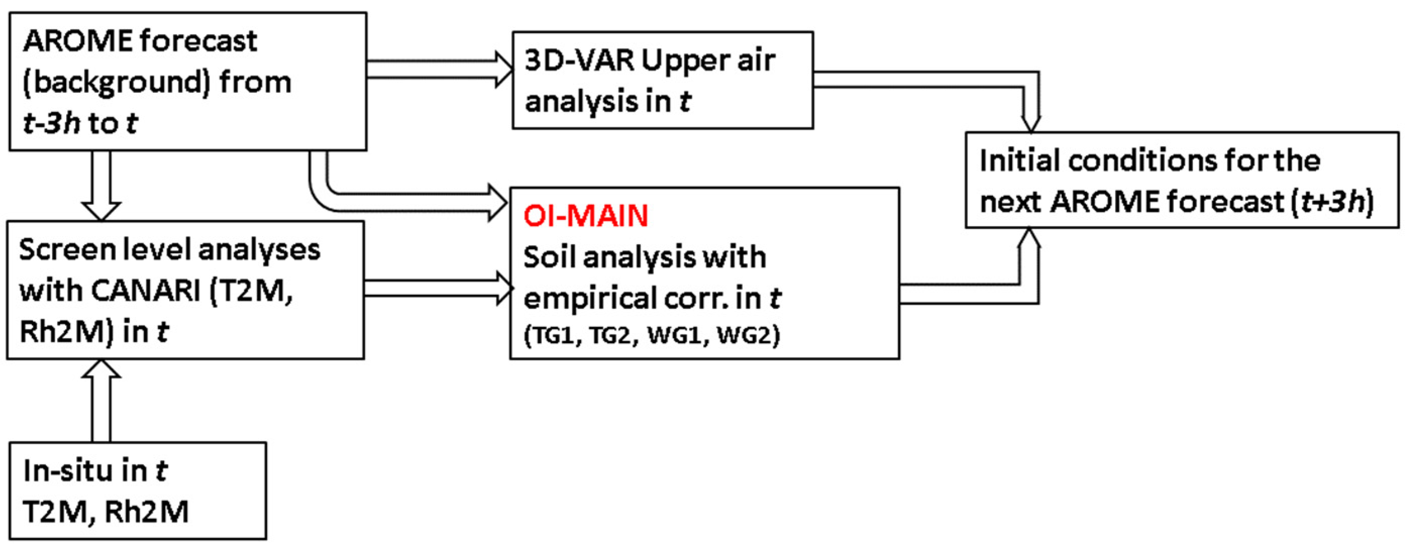
Optimal Interpolation (OI) is a widely used data assimilation technique that combines model background information with observational data to improve the initial state of a system. The surface assimilation based on OI consists of the following steps:

• Background state preparation: The AROME model forecast is run from t − 3h to t to provide the background land surface state.
• Observation processing: Quality control of the observations and interpolation and analysis of the 2-m temperature (T2M) and relative humidity (Rh2M) on a grid using CANARI (Code d’Analyse Nécessaire á ARPEGE pour ses Rejets et son Initialization), which is a univariate OI scheme [2,7].
• Surface and soil variables corrections: The corresponding correction of the surface and soil variables (temperature and water content) is done, which is called OI-MAIN [10]. This analysis is obtained independently at each grid point using the innovation between the pseudo-observations and the first guess of the screen-level elements.
• Initialization of the soil variables: The soil temperature and moisture are initialized using these innovations, taking advantage of the indirect impact between the 2-m elements and the soil variables.

Figure 2 shows the processing flow of the data assimilation of AROME using OI-MAIN for surface data assimilation.

In CANARI, several configuration parameters need to be defined. The background error standard deviations are set to 1.6 K for T2M and 18% for Rh2M. The observation error standard deviations are 1 K for T2M and 10% for Rh2M. The correlation length is set to 80 km for T2M and 85 km for Rh2M. In OI-MAIN, the background errors of soil temperatures (TG1 and TG2) are set to 2 K and 0.1 m³/m³ for soil water content (WG1 and WG2). We used the same configuration as presented in [6].

The effect and effectiveness of the method can vary greatly depending on the weather conditions. For a clear sky situation in a stable atmosphere, the assumptions of OI are valid, and the method improves the surface variables. On the other hand, under complex conditions, such as precipitation or a strong wind situation, OI struggles to apply properly due to spatial heterogeneity.

2.3. Surface Data Assimilation in AROME: Simplified Extended Kalman Filter

To further improve the representation of land surface processes, a more physically consistent approach is applied through the SEKF. When analyzing the soil variables, it is important to create the most accurate initial condition possible; therefore, dynamically changing coefficients are used during the SEKF. The analysis equation and the Kalman gain matrix (K) calculation using the Extended Kalman Filter are as follows:

$$x_a=x_b+\mathbf{K}{\left(y-\mathcal{H}{x}_b\right)}^{-1}$$

(1)

$$\mathbf{K}=\mathbf{B}{\mathbf{H}}^{\mathbf{T}}(\mathbf{H}\mathbf{B}{\mathbf{H}}^{\mathbf{T}}+\mathbf{R})$$

(2)

where x_a is the analysis (e.g., soil temperature and soil moisture, the so-called control variables), x_b is the result of a previous model run (first guess or background), y is the observations (e.g., 2-m temperature and relative humidity), and $\mathcal{H}$ is the nonlinear observation operator, which transforms the control variables from model space to observation space. By linearizing $\mathcal{H},$ we obtain the linearized observation operator H. K, the so-called gain matrix, which represents how much weight is given to observations versus the first guess when updating the analysis. B and R are the covariance matrices of background errors and observation errors, respectively.

In this study, we use the SEKF, a simplified version of the EKF, which means that the background error covariance matrix (B) does not change over time and R is constant. The elements of H (the so-called Jacobi matrix) are calculated using the finite difference method by perturbing each component x_j of the control vector x. The elements of the matrix H at a given time (i) can be written as follows:

$${\mathbf{H}}_{ij}={\displaystyle \frac{\partial y_i}{\partial x_j}}$$

(3)

The control variables we use are the TG and WG values at two levels: in the 0–1 cm thick layer close to the surface and in the root zone (0–2 m layer), while the observation variables are T2M and Rh2M. The Jacobian matrix can therefore be written as follows:

$$\mathbf{H}=\left[\begin{array}{cccc}{\displaystyle \frac{\partial \mathrm{T}2M}{\partial \mathrm{T}\mathrm{G}1}}& {\displaystyle \frac{\partial \mathrm{T}2M}{\partial \mathrm{T}\mathrm{G}2}}& {\displaystyle \frac{\partial \mathrm{T}2M }{\partial \mathrm{W}\mathrm{G}1}}& {\displaystyle \frac{\partial \mathrm{T}2M}{\partial \mathrm{W}\mathrm{G}2}}\\ {\displaystyle \frac{\partial \mathrm{R}\mathrm{h}2M}{\partial \mathrm{T}\mathrm{G}1}}& {\displaystyle \frac{\partial \mathrm{R}\mathrm{h}2M}{\partial \mathrm{T}\mathrm{G}2}}& {\displaystyle \frac{\partial \mathrm{R}\mathrm{h}2M}{\partial \mathrm{W}\mathrm{G}1}}& {\displaystyle \frac{\partial \mathrm{R}\mathrm{h}2M}{\partial \mathrm{W}\mathrm{G}2}}\end{array}\right]$$

(4)

In practice, the Jacobi expressions are generated by running the SURFEX model multiple times, from t − 3h hours to t for a total of n + 1 times, where n is the number of control variables. That is, in this case, there are 4 control variables plus a reference run, making it 5 runs. Each run starts with a small perturbation (10⁻³ or less) applied to the given control variable, which ensures the linearity of the observation H operator. Perturbation magnitudes in our configuration are set to 10⁻⁴ for WG and to 10⁻⁵ for TG. Since these are offline runs, external forcing files are required for SURFEX runs (i.e., radiation, precipitation, wind, humidity, temperature, and pressure) which are taken from AROME online forecasts at the lowest atmospheric model level of the model, which is currently 9 m above the surface.

For the ideal settings of B and R, several tests were performed, which are presented in Section 3.

Figure 3 shows the processing flow of the data assimilation of AROME using the SEKF for surface data assimilation. The main steps are as follows:

• Background state preparation: The AROME model forecast is run from t − 3h to t to provide the background land surface state.
• Observation processing: quality control of the observations and the interpolation and analysis of the 2-m temperature (T2M) and relative humidity (Rh2M) on a grid using CANARI.
• Calculate the Jacobian matrix: Numerically estimate H by perturbing the control variables and running SURFEX multiple times.
• Compute the gain matrix: K using the covariance matrices B and R in the Kalman Filter equations.
• Update the analysis: Combine the background state, gain matrix K, and the innovation to update the control variables.

3. Results

This section evaluates the performance of the SEKF assimilation. Section 3.1 examines the Jacobians of the observation operator at different analysis times and assesses their diurnal variability. In Section 3.2, a method is proposed to handle outlier Jacobians, thereby ensuring the linearity of the SEKF. Then, a case study is presented in which the soil temperature drops to an extremely low value, emphasizing the importance of properly setting the data assimilation parameters (Section 3.3). In Section 3.4, the examination and comparison of the analysis increments obtained by the SEKF and OI are presented. The forecast evaluation and verification are provided in Section 3.5.

3.1. Jacobians of Observation Operator

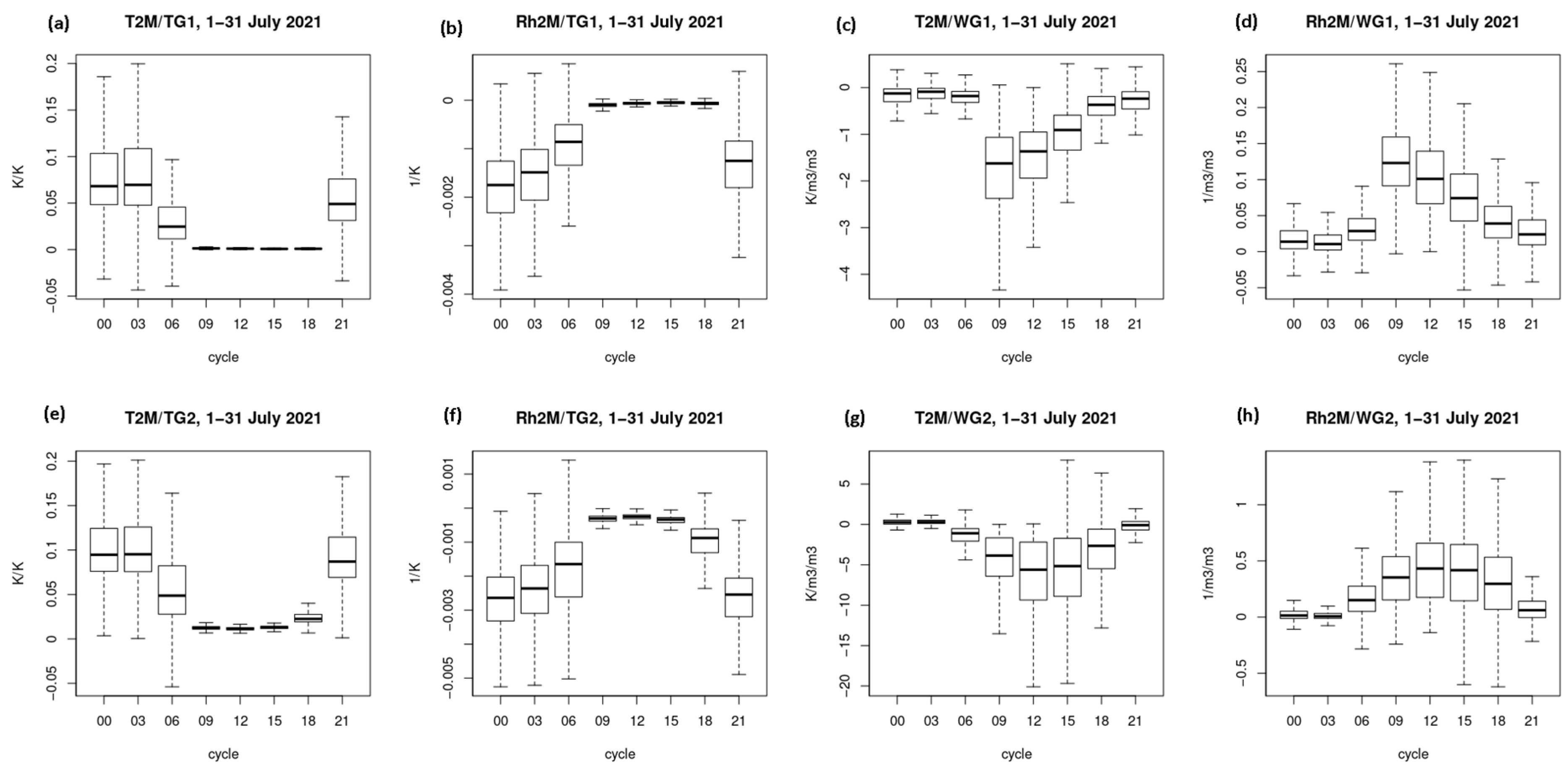
First, the Jacobian elements are calculated within our SEKF configuration, and their spatial variability is examined over the entire domain. Figure 4 shows the boxplots for the Jacobians of the observation operators for ${\displaystyle \frac{\partial T2M}{\partial TG1}}$, ${\displaystyle \frac{\partial T2M}{\partial WG1}}$, ${\displaystyle \frac{\partial Rh2M}{\partial TG1}}$, ${\displaystyle \frac{\partial Rh2M}{\partial WG1}}, {\displaystyle \frac{\partial T2M}{\partial TG2}}$, ${\displaystyle \frac{\partial T2M}{\partial WG2}}$, ${\displaystyle \frac{\partial Rh2M}{\partial TG2}}$, and ${\displaystyle \frac{\partial Rh2M}{\partial WG2}}$ calculated over the whole domain and averaged for July 2021 for the different analyses times (0, 3, 6, 9, 12, 15, 18, and 21 UTC). The top row of Figure 4 shows the Jacobians for the superficial soil layer, while the bottom row indicates the Jacobians for the root zone. Similar but slightly smaller Jacobian coefficients were also obtained for winter.

The response of T2M to soil temperature is mainly positive, meaning that an increase in the soil temperature leads to an enhancement in the 2-m temperature. However, the response of T2M to soil moisture is more complex and can be negative, because an increase in soil moisture often reduces T2M, as increased evapotranspiration through wetter soil decreases the sensible heat flux. In contrast, in very dry conditions, adding soil moisture can initially warm T2M due to enhanced heat conduction in the soil.

The response between Rh2M and soil temperature is negative, while that between Rh2M and soil moisture is positive, indicating the natural interaction between sensible and latent heat flux effects. Both T2M and Rh2M responses exhibit relatively larger temporal variation in the superficial layer, as expected from rapid near-surface thermal and moisture changes.

It is also noticeable that the Jacobians are larger in the root zone than near the surface, which results in a stronger impact on the analysis due to delayed land surface–atmosphere interactions.

Examining the diurnal cycle reveals different responses of screen-level parameters to changes in soil moisture and soil temperature. The influence of soil moisture is more pronounced at night, whereas the effect of soil temperature is stronger during the day. Higher soil moisture provides more water for evaporation, enhancing Rh2M in daytime, and the increased water vapor provides a cooling effect near the surface. At night, however, without solar radiation, the evaporation is reduced. During nighttime, the energy exchange is dominated by sensible heat flux from the soil, which has a strong impact on T2M. In contrast, during the day, the soil temperature has a less indirect influence on T2M, as much of the available energy is consumed by the latent heat flux.

The distinct diurnal effects highlight the importance of a 3-hourly assimilation cycle, in which the Jacobians used in the SEKF are recalculated, as opposed to OI-MAIN, where coupling coefficients are fixed.

3.2. Outlier Jacobians—Checking the Linearity of the SEKF

One of the difficulties of using the SEKF as a data assimilation technique is that the Jacobian elements become excessively large. In these cases, the linear assumption in the SEKF calculation is questionable. To prevent numerical instability and mitigate nonlinear effects, thresholds are imposed on the Jacobians. In the ECMWF, these thresholds are 50 K/m³/m³ for ${\displaystyle \frac{\partial T2M}{\partial WGi}}$ and 500%/m³/m³ for ${\displaystyle \frac{\partial Rh2M}{\partial WGi}}$ [28].

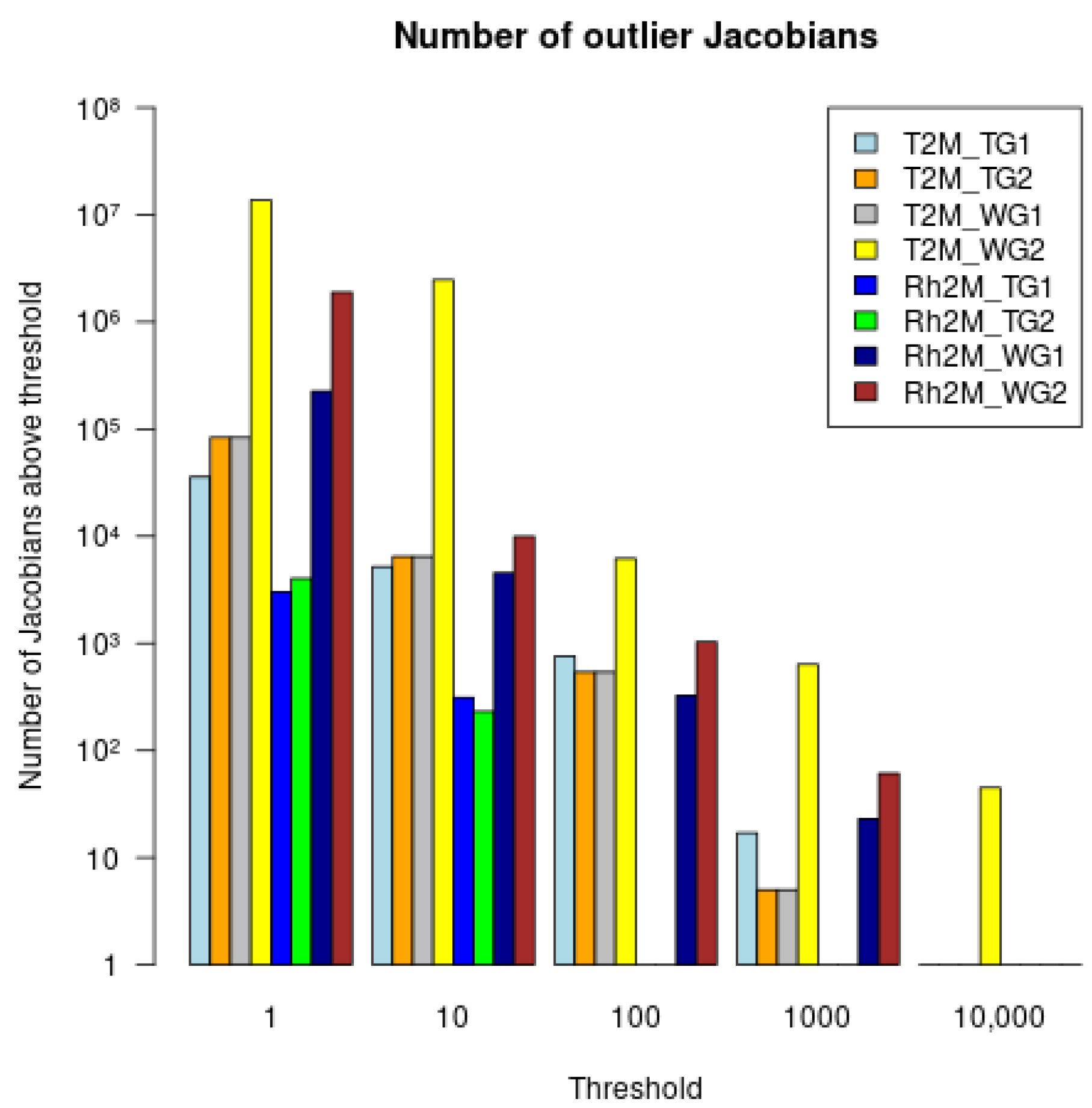
To evaluate the likelihood and severity of nonlinear cases, the number of large Jacobians for all control variables in July 2020 is shown in Figure 5. With Jacobians larger than 1, the linear approximation may already be violated. The highest number of outlier Jacobians was observed for ${\displaystyle \frac{\partial T2M}{\partial WG2}}$, which even reached 10,000 K/m³/m³. Most of the large Jacobi magnitudes are primarily influenced by soil moisture (WG1 and WG2) perturbations, in contrast to soil temperature (TG1, TG2). The differences are likely due to the different physical processes that soil moisture and soil temperature influence in the surface atmosphere system. Soil moisture significantly influences the latent heat flux due to evaporation and transpiration. While soil temperature primarily affects sensible heat flux, it also indirectly influences evapotranspiration, although its impact is less significant compared to that of soil moisture.

Furthermore, regardless of the selected threshold, the number of outliers was orders of magnitude higher for ${\displaystyle \frac{\partial T2M}{\partial WG2}}$ than for any other Jacobians. This indicates that the SURFEX shows a high sensitivity of T2M to the root-zone soil moisture (WG2), and large corrections in soil moisture during the analysis can cause large discrepancies in T2M.

In SURFEX 8.0, it is hard-coded that Jacobians smaller than 1 guarantee the linearity of the system. However, this constraint is very strict: As it reaches the threshold at many points, the SEKF cannot be applied in these cases. In contrast, our target was to keep the large but valid Jacobians. Therefore, positive and negative perturbations for all control variables were calculated, and the linearity of the Jacobians was checked with the following conditions obtained by [29]:

|H⁺ + H⁻| > 0.2·(|H⁺| + |H⁻|)/2.0

(5)

If (5) is true, the system becomes nonlinear, and H must be equal to 0. The Jacobian filtering involves identifying and eliminating Jacobian terms that are considered unreliable or suspect. This process helps improve the stability and accuracy of the calculations.

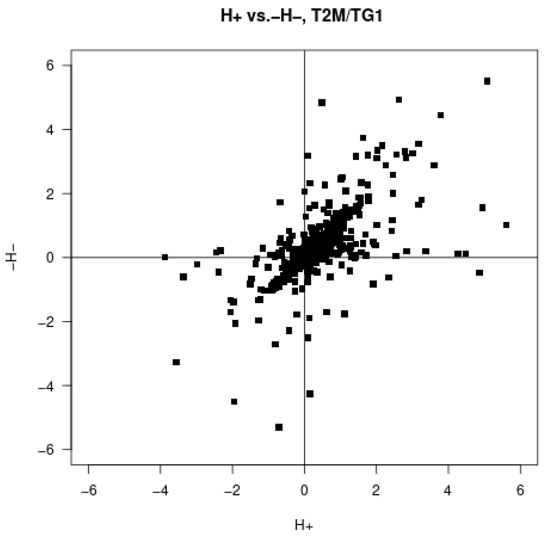
The ratio of positive and negative Jacobians is evaluated for ${\displaystyle \frac{\partial T2M}{\partial TG2}}$ in Figure 6. Elements along the diagonal are considered to be good, even if they are larger than 1, as this indicates acceptable linearity for SEKF assimilation. There are a lot of points where sensitivity of the T2M to the positive and negative perturbations of soil temperature can differ significantly, which can lead to asymmetric responses between the sensible and the latent heat fluxes. The positive perturbation increases the sensible heat flux, which is amplified if the soil is too dry and less energy is used for evaporation, causing T2M to increase. On the other hand, negative perturbation reduces the sensible heat flux, but the latent heat flux remains constrained in the dry soil, and, therefore, T2M may not decrease significantly. This can occur when the soil moisture is close to the wilting point. Similar behavior of the Jacobians was demonstrated by [6]. Under such dry conditions, the Jacobian elements associated with soil moisture become very small or even negligible, reflecting the weak or absent sensitivity of screen-level variables to changes in root-zone soil moisture, and the transpiration remains negligible.

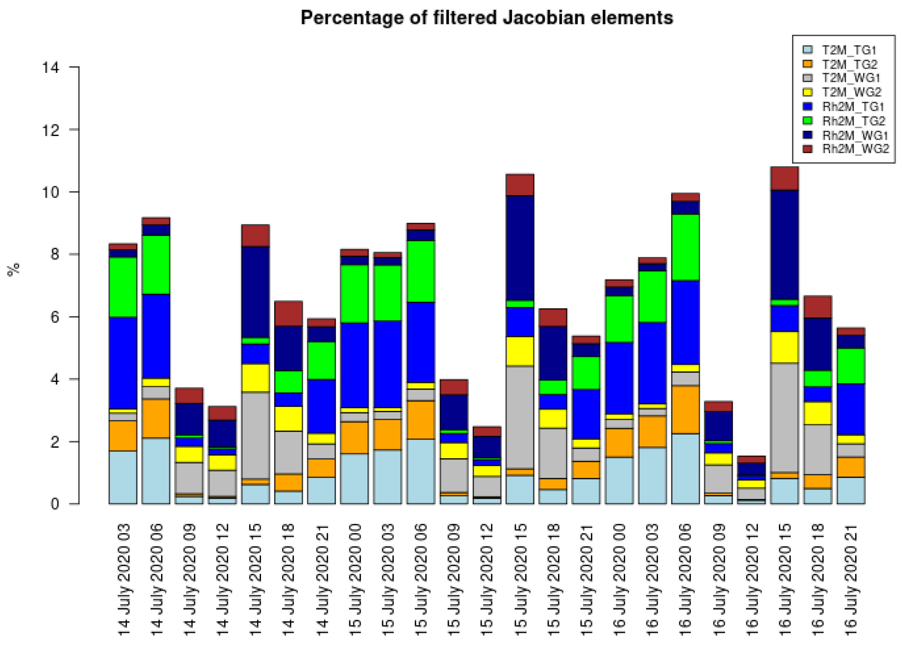
The linearity check ensures that the Jacobians accurately describe the perturbation-based sensitivities and remain valid. With the linearity checking, 2–12% of the Jacobians were dropped (Figure 7). The ratio of the rejected value was lower at middays and higher in the nights and mornings. At midday, the land–atmosphere system behaves more linearly due to stronger turbulence, while at nights, higher rejection happens due to the stable boundary layer and nonlinear radiative cooling. The ratio of rejected Jacobians for relative humidity is higher than for temperature, except at 15 UTC, when they are roughly equal and the highest. Relative humidity has a strong diurnal cycle, being lower in the afternoon as the heating reaches its peak, which leads to strong turbulence or instabilities. This can rapidly change the screen-level parameters, and the linear approximations cannot be valid. Nonlinearity is further amplified in these cases as WG2 has a delayed response to surface forcing, making filtering essential to maintain physical realism.

The filtered points were found randomly in the area of the domain. By using the linearity check, the analyzed total water content could differ by up to 10–20%.

3.3. Soil Temperature Problem in Winter Experiment

A winter experiment was conducted from 20 November to 17 December 2019 (with a spin-up period from 11 November) using the SEKF in the AROME model. Spurious and unrealistic TG1 and TG2 values were detected towards the end of the experimental period. At certain points, these values dropped below 200 K and even reached as low as 1–2 K.

The left map on Figure 8 shows the areas with extremely low (below 198 K) TG2 values, particularly in the Alps, while the diagram on the right illustrates the time evolution of TG2 at the marked point. In the last third of the period, TG2 became unacceptably low.

It was hypothesized that this issue was caused by spurious large Jacobians, prompting a linearity check of the Jacobians in the next experiment. Under snow conditions, Jacobians can increase, causing a strong Kalman gain [28], leading to downward increments in TG2. Although the Jacobians evaluated in a reasonable range, and the new run slightly corrected the TG2 analysis, the values later became false in the target point.

Further investigation continued, but none of them provided a satisfactory solution to this problem. Neither the blacklisting of the neighboring SYNOP stations nor modifications to the SEKF equations (Jacobians, innovations, and increments) produced reliable results. Finally, it turned out that the error was closely related to the assimilation settings, especially the observation errors (XERROBS), background errors (XSIGMA), and the perturbation sizes (XTPRT). The background errors for surface and deep soil moisture content were set to XSIGMA × (WG_fc − WG_wilt), with WG_fc and WG_wilt being the volumetric water content at field capacity and at the wilting point, respectively, both of which depend on soil texture [23].

Several tests were conducted with different assimilation settings for the winter period (

Table 1. Experiments with different assimilation settings.

	EXP1	EXP2	EXP3	DEF	ECM	ECM_B	EXP4
XERROBS (T2M, Rh2M)	0.5 K, 0.2	0.5 K, 0.2	1.0 K, 0.4	1.0 K, 0.1	1.0 K, 0.04	1.0 K, 0.04	1.0 K, 0.07
XSIGMA (WG2, WG1, TG2, TG1)	0.15 m3/m3, 0.1 m3/m3, 2 K, 2 K	0.15 m3/m3, 0.1 m3/m3, 2 K, 2 K	0.15 m3/m3, 0.1 m3/m3, 2 K, 2 K	0.15 m3/m3, 0.1 m3/m3, 2 K, 2 K	0.15 m3/m3, 0.1 m3/m3, 2 K, 2 K	0.01 m3/m3, 0.01 m3/m3, 1 K, 1 K	0.15 m3/m3, 0.1 m3/m3, 2 K, 2 K
XTPRT (WG2, WG1, TG2, TG1)	10−4, 10−4, 10−5, 10−5	10−3, 10−3, 10−4, 10−4	10−4, 10−4, 10−5, 10−5	10−4, 10−4, 10−5, 10−5	10−4, 10−4, 10−5, 10−5	10−4, 10−4, 10−5, 10−5	10−4, 10−4, 10−5, 10−5
TG2 acceptable?	NO	NO	YES	YES	NO	YES	YES

).

From the table, it can be seen that the value of XERROBS is crucial. The only difference between EXP1 and EXP3 was in the XERROBS values, resulting in a very different quality of TG2. In EXP1, the lower observation error for both T2M and Rh2M increased the influence of the observations in the analysis, resulting in an unbalanced surface assimilation of the control variables. In EXP2, the perturbation sizes (XTPRT) were adjusted, while all other settings remained the same as EXP1. However, TG2 still became unacceptable. DEF refers to the experiment using the default values, in which the soil moisture and temperature analysis and forecast were obtained to be acceptable. In EXP4, the XERROBS for Rh2M was tuned a bit compared with DEF, leading to better results. ECM represents the run with XERROBS applied as used in ECMWF, while XISIGMA remained the same as in DEF. On the other hand, ECM_B was similar to ECM in terms of XERROBS, but XSIGMA was reduced to the setting used in ECMWF. While ECM produced false TG2 values, these were resolved in ECM_B. In the following, we focus on the results obtained with the EXP4 settings, as they provided slightly better verification results compared to DEF.

3.4. Examination of the Analysis Increments

Next, we compare the differences between the OI and SEKF analysis increments. Figure 9 shows the analysis minus guess (A-G) increments for soil temperature and soil moisture at different analysis times, averaged for the entire study period and across all grid points within the domain.

The temperature increments were predominantly negative with both methods, with a larger increment occurring at night and smaller during the day. This pattern corresponds with our expectation, as the AROME tends to overestimate the near-surface temperature during the summer period, mainly at night. For OI-MAIN, the TG2 increments were smaller and more consistent compared to the SEKF. In contrast, the TG1 increments presented opposite behavior, as the SEKF had a more limited impact on the superficial soil temperature. This suggests that updating soil temperature by the SEKF may favor deeper layers over the surface.

Regarding soil moisture, the WG1 increments were large and positive during the day in the case of OI-MAIN, likely reflecting a stronger correction of surface drying. On the other hand, the WG2 increments were negative for daytime and positive for nighttime for the SEKF. This behavior indicates that the SEKF is able to more dynamically redistribute moisture corrections between layers, especially by increasing nighttime moisture content while decreasing daytime values.

In winter, the SEKF produced a large negative soil moisture increment, while with OI-MAIN, almost no increment was obtained, particularly for WG2. This suggests that the SEKF responded more actively to the 2-m observations, indicating drier conditions near the surface leading to reduced soil moisture. During winter, when the soil moisture changes are small, the SEKF can still adjust the soil moisture state through the Jacobians, while OI-MAIN is less sensitive to small changes in soil moisture and tends to assume more stable or neutral estimates. We have to note OI-MAIN limiters during strong winds or cloudy conditions. In these situations, its impact is reduced, because it relies on static error matrices, which do not account for dynamic atmospheric changes.

For soil temperature, both methods produced positive increments during the day and negative increments at night for both soil layers. This is consistent with the thermal properties of drier soil, which has lower heat capacity, providing rapid cooling at night and warming during the day.

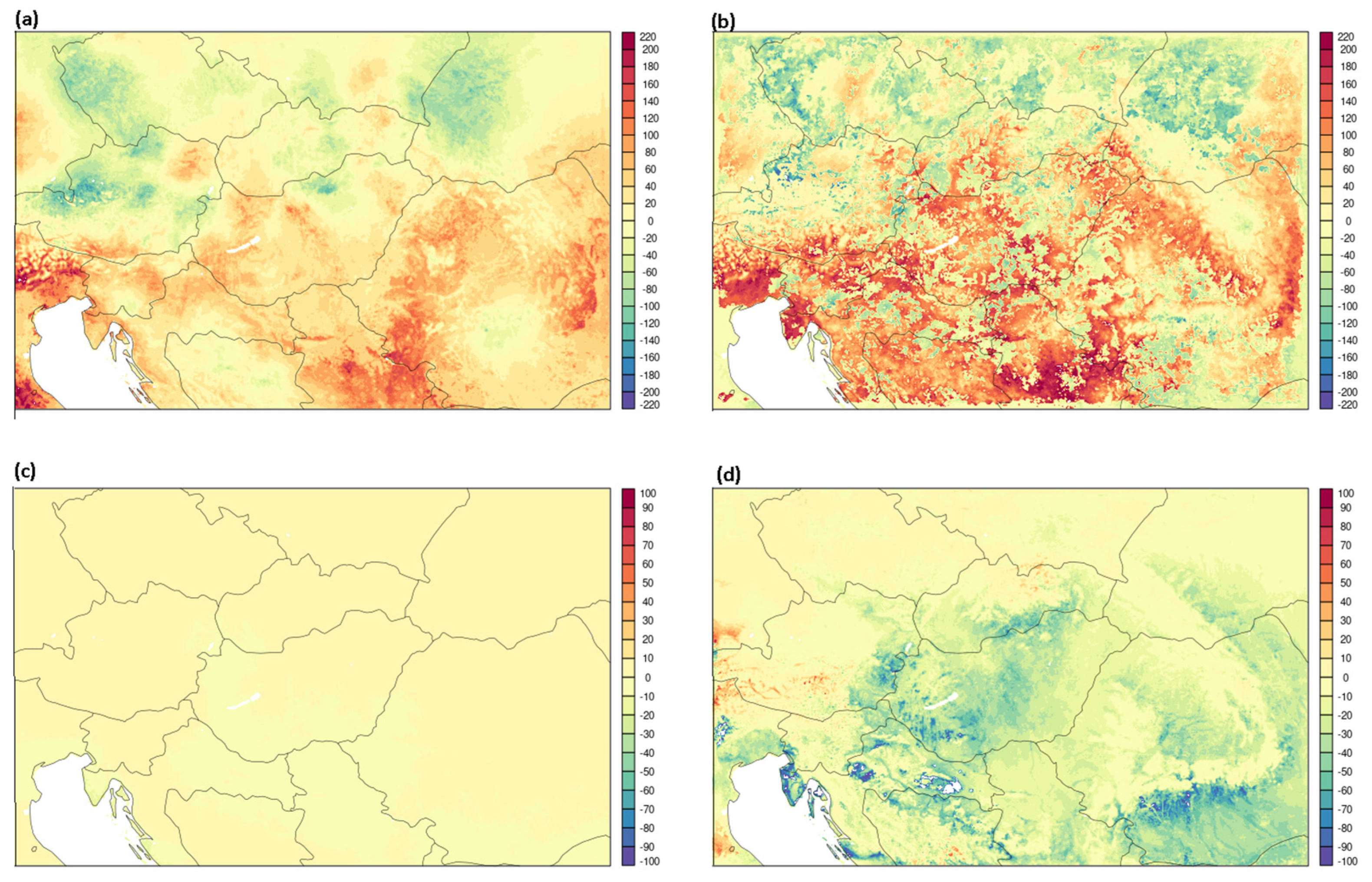
The previously mentioned features in soil moisture increments are also visible spatially (Figure 10), although some variations are climatically controlled combined with soil texture patterns. In summer, the spatial structure of the soil moisture increments was similar for the SEKF and OI-MAIN, as positive increments were experienced in the central and southern part of the area and negative in the northern part. The positive increments reached up to 200 mm in many areas, while the negative ones were more moderate. Compared to the SEKF, the increments produced by OI-MAIN were smoother and smaller. In contrast, the SEKF obtained more fine-scale variability.

In January, the soil moisture increments were significantly lower and more restrained than in July, with values even approaching zero in the case of OI-MAIN. This is in parallel with the results presented in Figure 9, where OI-MAIN showed minimal soil moisture increments in winter. However, the SEKF continued to produce notable increments, which were predominantly negative, indicating drying of the soil.

3.5. Forecast Evaluation

Screen-level parameters were verified for winter (December 2021–February 2022) and spring (March–May 2022) based on model forecasts provided by OI-MAIN and the SEKF. The winter of 2021/2022 was characterized by mild and dry conditions, with frequent cold anticyclonic periods. In these kinds of weather situations, the influence of the ground on the near-surface air layers is mainly strong. In spring, the cool weather continued, resulting in a slightly cooler season than usual. Regarding precipitation, the individual months showed significant variability. There was a significant lack of precipitation in March and May; in contrast, April was rainier than usual.

Point-wise verification was conducted over Hungary using SYNOP observations. Scorecards were generated using the HARP (Hirlam-Aladin R Package for verification version 0.2.2), which is a well-structured tool to compare numerical weather prediction models across different metrics [30]. Additionally, a bootstrap resampling hypothesis was applied to determine which model performs better for different scores and whether the differences are statistically significant [31].

First, the forecast-observation pairs are computed. Then, they are randomly sampled with a replacement to create a bootstrap sample and calculate the performance metric. This resampling process is repeated n times to generate the distribution of the metric. This is followed by computation of the confidence intervals and comparison of the distributions between models to test the statistical significance. However, a potential issue arises in bootstrapping when the data are serially correlated (autocorrelation), either in time or in space [32]. In order to obtain a representative statistic, we need to ensure that the serial correlations are handled. In our case, we mitigated the effect of autocorrelation by using n = 100 iterations and 5-day blocks for resampling to reduce the impact of autocorrelation.

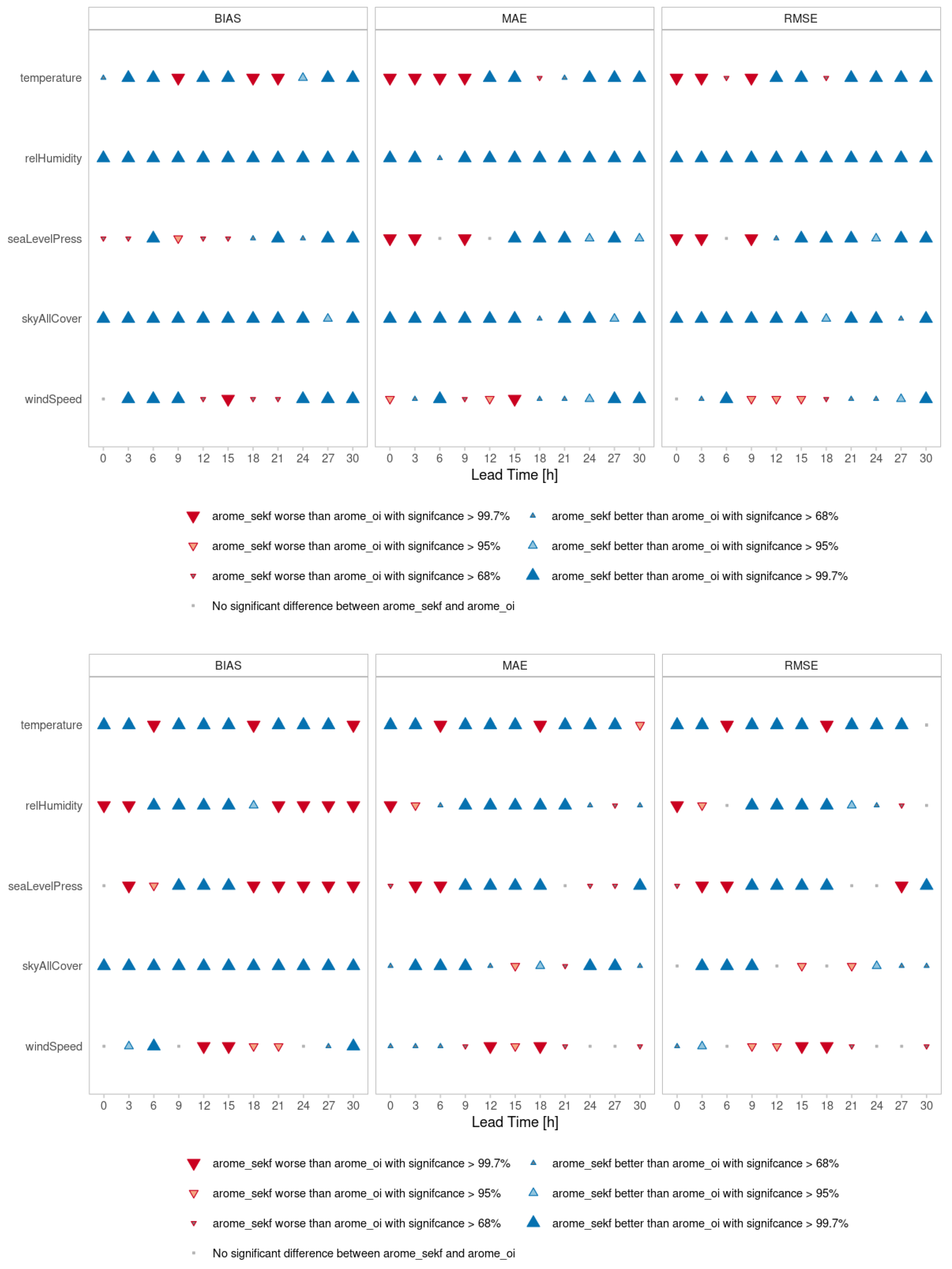
Figure 11 illustrates the scorecards for various statistics of screen-level parameters, including bias, mean absolute error (MAE), and root mean square error (RMSE) for T2M, Rh2M, mean sea level pressure (MSLP), cloud cover, and 10-m wind speed. These metrics were evaluated up to a +30 h lead time, averaged over 3-month periods for winter (top part of Figure 11) and spring (bottom part). The blue triangles indicate improvements for the SEKF compared to OI-MAIN, with their size reflecting the level of statistical significance. Only the 00 UTC runs were evaluated in this study.

In winter, there were notable improvements for the SEKF at the 99% confidence level across various parameters:

• Rh2M and cloud cover showed significant improvements in bias, MAE, and RMSE for all forecast ranges.
• For T2M, the SEKF showed improvements in bias except at +9, +18 and +21 h, while the MAE and RMSE initially deteriorated in the first hours but later improved.
• For the MSLP, the results showed deterioration in the MAE and RMSE in the first hours, followed by improvement later in the forecast period.
• Total cloudiness improved significantly across all metrics, including bias, the MAE, and the RMSE, indicating that the SEKF provided more accurate cloud cover predictions compared to OI-MAIN.
• The 10-m wind speed deteriorated during the day but showed improvement at night.

In spring, the results were slightly worse compared to winter, mainly in terms of bias for Rh2M and in all scores for the 10-m wind speed. Specifically, the improvements observed in winter were not as pronounced in spring.

• Rh2M showed a deterioration in bias at nights and improvements during the day.
• For the T2M and 10-m wind speed, the behavior in spring was similar to that observed in winter. In the case of the 10-m wind speed, the quality of the SEKF declined across all evaluated metrics (bias, MAE, and RMSE) compared to the improvements seen in winter. In contrast, the T2M showed more consistent behavior, maintaining similar levels of accuracy in both winter and spring.
• The bias of total cloudiness was also better, which suggests that the SEKF was effective in producing more accurate forecasts of cloudiness, both in winter and spring.

These results suggest that the seasonal variability in atmospheric conditions might influence the forecasts produced by the SEKF. As mentioned earlier, the winter and spring were dominated by dry and cool anticyclonic weather patterns, during which the soil had a strong impact on the near-surface atmospheric layers. Under these weather conditions, the SEKF improves the forecast of near-surface parameters and their diurnal cycle compared to OI-MAIN. This suggests that the SEKF is particularly effective when land–atmosphere interactions play a dominant role. On the other hand, under different meteorological conditions, the impact of the SEKF is more limited.

4. Discussion

Our study demonstrates that the Simplified Extended Kalman filter (SEKF) method improves the assimilation of 2-m temperature (T2M) and relative humidity (Rh2M) compared to the currently operational OI-MAIN system. These improvements are most pronounced in spring and summer, especially in the root-zone soil moisture variables. The SEKF’s ability to dynamically update sensitivities based on the current state results in more physically consistent corrections, whereas the OI system applies static, climatologically-based increments.

4.1. Diurnal Variability of Jacobians and Sensitivity

Figure 4 shows that the Jacobians in the SEKF exhibit strong diurnal and seasonal variations, reflecting changes in boundary layer depth and land–atmosphere coupling. This time dependence enables the SEKF to apply more accurate corrections during periods of strong coupling (e.g., early morning and mid-afternoon), a feature completely absent in OI-MAIN. The Jacobian filtering behavior, illustrated in Figure 7, shows a peak in filtering activity at 15 UTC, indicating when the system actively suppresses updates due to nonlinearities. This is consistent with the findings of [6,29], who noted these time-dependent sensitivities (both in pattern and magnitude) of SEKF systems, although neither analyzed diurnal Jacobian variability in detail.

This study introduced a linearity check method based on the symmetry of Jacobian responses to positive and negative perturbations (Figure 5 and Figure 6). Linearity was evaluated separately for each variable and soil layer, allowing selective filtering: A Jacobian could be excluded in one layer but retained in another. About 60% of the filtered Jacobians were linked to the superficial layer, while only 20% affected both layers, suggesting that most nonlinearities were layer-specific and localized. Previous studies typically discarded Jacobians exceeding a threshold without testing linearity [5,6,33,34]. Some tried to reduce extreme values either by averaging symmetric perturbations [35] or reducing values by an adaptive method [36] but these methods do not eliminate nonlinear responses.

In [28], various filtering strategies were tested. In the strictest setup, the entire control vector (soil moisture, soil and snow temperature) was discarded if any Jacobian exceeded the threshold. More relaxed approaches applied filtering by variable group (e.g., rejecting only soil moisture). The strict configuration caused local degradation in T2M, especially over data-sparse regions such as Siberia.

4.2. Differences Between SEKF and OI Soil Variable Increments

There are seasonal differences in how the SEKF and OI update soil moisture and temperature variables (Figure 9 and Figure 10). In winter, OI applies minimal increments to soil moisture due to low latent heat fluxes; however, in summer, OI shows strong positive increments. The SEKF contributes more varied and spatially structured increments in both seasons.

For soil temperature in winter, however, OI actively applies larger positive increments in TG1 than the SEKF, while in summer, OI continues to dominate TG1 updates, whereas the SEKF applies stronger cooling in TG2. The SEKF dominates TG2 updates across all seasons, pointing to a stronger coupling with deeper soil variables [5,6,18]. This behavior arises from the fact that the SEKF dynamically evolves the Jacobians, allowing information from 2-m observations to propagate downward into deeper soil layers. In contrast, OI-MAIN relies on static error matrices, which assign greater weights to the surface layers, thereby limiting its capacity to transfer observational information deeper into the soil.

These deeper-layer corrections reflect the SEKF’s ability to adapt based on diurnal and seasonal sensitivity structures, particularly under stronger land–atmosphere coupling conditions.

4.3. Forecast Performance

The forecast evaluation (Figure 11) confirms the SEKF’s advantage for Rh2M and T2M, particularly during nighttime and in winter. In spring, the SEKF maintains its advantage for Rh2M during most hours, although its performance dips around the early morning hours for T2M. For wind speed, the SEKF performs better at night but shows mixed results during midday in spring. These variations align with the observed diurnal Jacobian structure and soil increment behavior. The consistency between diagnostic (Jacobians and increments) and prognostic (forecast scores) indicators validates the SEKF scheme’s process-level advantages.

Seasonal differences in performance can be attributed to shifts in the dominant weather regime and the underlying soil state. The wintertime improvements stem largely from OI’s inactivity, whereas in spring, the SEKF competes with reactivated OI-MAIN tendencies. The daytime forecast performance for the SEKF also reflects its ability to capture peak surface flux periods better than the climatologically fixed OI.

4.4. Improvements over Existing Analysis

Our results confirm earlier findings (e.g., Refs. [5,6,17]) that Kalman-based methods offer a more physically consistent alternative to static OI schemes. However, our implementation is novel in that it uses station-based observations with a 3-hourly cycling frequency and explicit Jacobian filtering. This is not commonly done in operational NWP systems, as typically a 6-h cycle is employed [6,17,18,19,33]. This allows us to examine time-dependent sensitivities in more detail and link them to observed forecast improvements.

Compared to studies like [6], which demonstrated improvements in screen-level variables by using the SEKF in SURFEX, our implementation builds on this by explicitly analyzing the diurnal structure of the Jacobians and extending the comparison to soil variables. Our finding that the SEKF applies stronger corrections to deeper layers than OI, especially under high-coupling conditions, is in line with the sensitivity analyses of [37], though we use deterministic Jacobian filtering rather than ensemble perturbations.

The observation and model errors were also evaluated within our system. The optimal values were found to be consistent with those reported in previous studies [6,33]. In [17], sensitivity analysis was performed with the observation errors approximately doubled, thereby reducing the average step size of root-zone soil moisture analysis by approximately 60%. Furthermore, Ref. [17] demonstrated that tuning of the observation errors was important to create the operational surface assimilation settings at the ECMWF.

4.5. Methodological Limitations and Sensitivities

Despite its advantages, the SEKF’s performance is limited by its use of static background (B) and observation (R) error covariances. These fixed settings can lead to misweighting of updates during rapidly changing surface conditions, especially in spring. Additionally, the size of the perturbation used to compute the Jacobians (XTPRT) and the filtering threshold can significantly affect the stability and realism of increments.

As shown in the parameter tuning tests (Table 1), lowering the background error standard deviation (XSIGMA) can reduce unphysical responses in deeper layers such as TG2. A lower XSIGMA enhances the influence of the background in the analysis. Using XERROBS from the ECMWF (ECM experiment), false TG2 values were observed at the end of the period, proving that both T2M and Rh2M observation errors are crucial in the SEKF. If these values are too low, they can lead to an imbalance in the system. While ECM used XERROBS values similar to the ECMWF and resulted in unstable TG2 behavior, the ECM_B configuration with reduced XSIGMA restored physical consistency. This result indicates that XSIGMA in addition to XERROBS is an important parameter for maintaining system stability and enhancing SEKF accuracy. Similarly, the perturbation size (XTPRT) affects the linearity of Jacobian estimates: If it is too small, numerical precision errors occur; if too large, nonlinearities dominate [38]. These results emphasize the need for balanced parameterization in SEKF design, as it noted by [33].

It should also be noted that the SEKF is ten times slower than OI-MAIN. The increased computational cost of the SEKF, due to its dynamic assimilation process and the calculation of the Jacobians, results in longer processing times compared to the more straightforward static error matrix approach used in OI-MAIN.

5. Conclusions

The SEKF method provides a meaningful improvement over OI-MAIN in the assimilation of 2-m variables and land surface states. Its state-dependent sensitivity updates allow it to capture diurnal and seasonal variability in land–atmosphere coupling more effectively. These advantages translate into improved forecast skill, particularly for Rh2M, and deeper soil moisture states where OI lacks responsiveness.

The SEKF system was implemented into the AROME-Hungary operational chain with full cycling and diagnostic filtering at the HungaroMet Hungarian Meteorological Service in June 2022. Despite its increased computational complexity, the system remained numerically stable and provided consistent improvements without introducing unphysical behavior. Its ability to selectively suppress updates under strong nonlinearity contributes to its robustness.

The next phase of the work will involve MetOp ASCAT-B and C satellite soil moisture measurements [39], which will provide additional observational data to further enhance the accuracy of soil moisture analysis and forecasts [13,16,18,19,21]. The integration of these satellite-based measurements will improve the monitoring of soil moisture conditions, mainly in regions where in situ data are sparse. Additionally, the representativeness of satellite measurements is also better, further enhancing the accuracy of surface analyses and forecasts.