A Novel Approach to Understanding the Complexity of Precipitation

Abstract

One of the most challenging tasks in studying precipitation is quantifying how the complexities of individual components contribute to the overall system complexity. To address this, we employed information measures based on Kolmogorov complexity (KC), specifically the Kolmogorov complexity spectrum (KC spectrum) and the Kolmogorov complexity plane (KC plane). We applied these measures to monthly time series data, both measured and simulated by the EBU POM regional climate model, spanning the period from 1982 to 2005 for Sombor (45.78° N, 19.12° E) in Serbia. The variables analyzed included precipitation—a complex physical system—and its individual components: mean temperature, minimum and maximum temperatures, humidity, wind speed, and global radiation. By applying the listed measures to all time series, we calculated normalized KC spectra for each position in the KC plane, displaying interactive master amplitudes against individual amplitudes. We proposed a simplified four-step method to compute the relative change in complexities within the overlapping area beneath the KC spectra. Our results facilitated a discussion on the relationship between the complexity of precipitation and that of its individual components.

1. Introduction

Understanding precipitation patterns is essential for a wide range of fields, including meteorology, agriculture, and climate science. However, traditional approaches to studying precipitation often depend on linear models and historical data analysis, which can fail to capture the intricate interactions and dynamic complexities inherent in weather systems.

1.1. Preliminaries

Precipitation is a multifaceted phenomenon that exhibits several key characteristics of a complex system: (1) Interconnected processes: Cloud formation is a prime example, where atmospheric conditions, aerosol presence, and temperature gradients interact to influence precipitation development. (2) Atmospheric dynamics: Wind patterns, temperature gradients, and humidity levels are crucial in shaping cloud development and precipitation distribution. These factors interact in complex ways to determine where and when precipitation occurs. (3) Feedback loops: Processes such as evaporation and condensation create feedback loops that significantly affect precipitation intensity and distribution. For instance, increased evaporation can lead to more intense precipitation events. (4) Nonlinearity: Small changes in atmospheric conditions can lead to substantial variations in precipitation patterns, illustrating the system’s sensitivity to initial conditions. (5) Emergence: The collective behavior of atmospheric particles and processes gives rise to emergent properties, such as complex precipitation patterns, which cannot be predicted solely from the characteristics of their components. Note that this emergent behavior is a hallmark of complex systems. (6) Adaptation and sensitivity: Precipitation systems are susceptible to fluctuations in global climate patterns, such as El Niño and the North Atlantic Oscillation. These fluctuations can profoundly impact regional precipitation patterns, leading to significant alterations in local hydrological cycles. (7) Scale and hierarchy: Precipitation phenomena unfold across multiple spatial and temporal scales, ranging from localized thunderstorms to large-scale global climate patterns. To fully grasp precipitation, it is essential to consider these diverse scales and their intricate interactions.

Therefore, precipitation constitutes a complex physical system characterized by interconnected processes, nonlinear dynamics, emergent properties, heightened sensitivity to environmental changes, a hierarchical structure spanning multiple scales, and an inherently interdisciplinary nature that necessitates a comprehensive, multifaceted approach to its study.

1.2. Complexity Versus Randomness

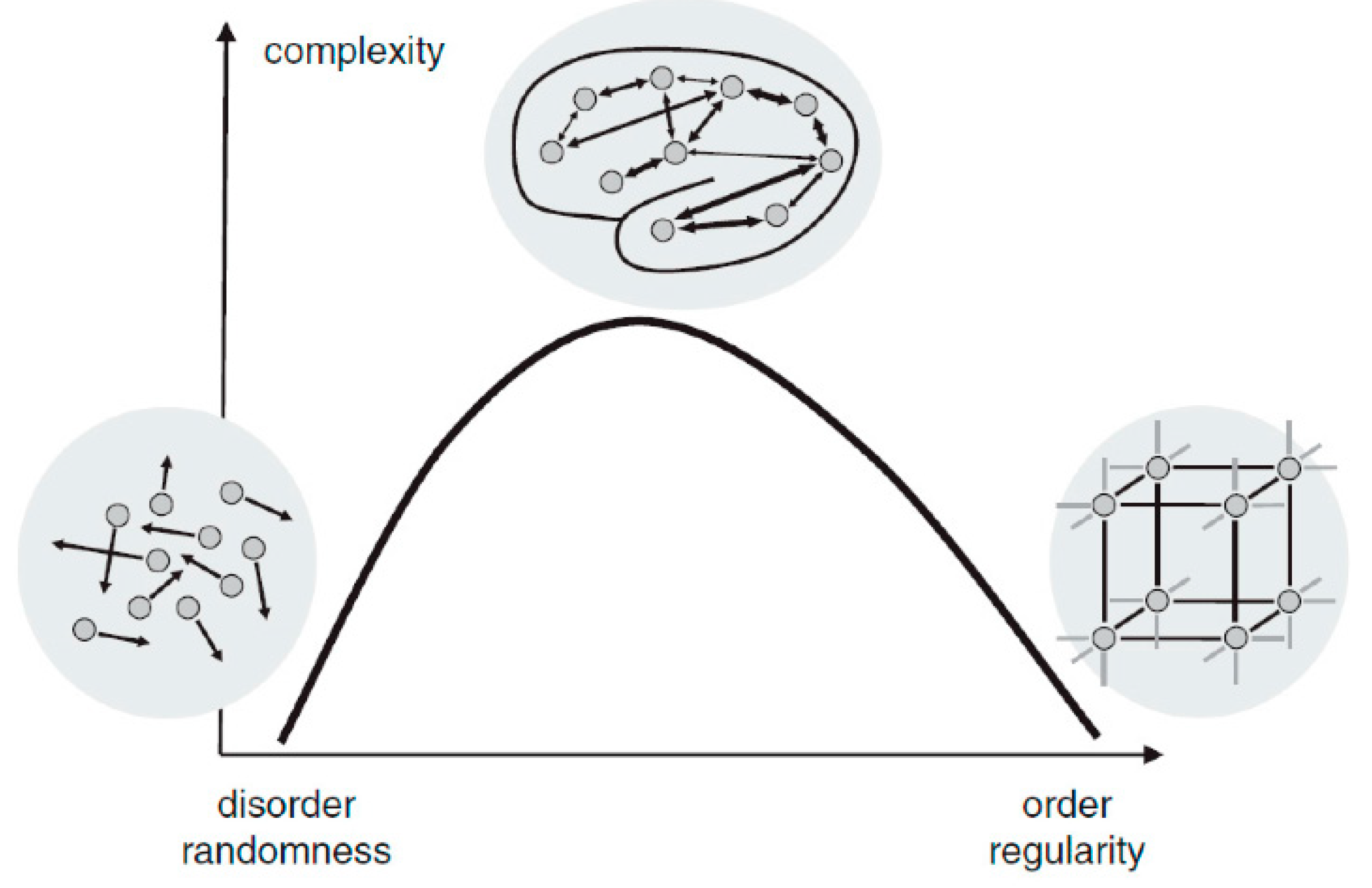
In the previous subsection, we discussed the properties of precipitation as a complex system. When considering the complexity of this system and its implications for precipitation, two key points should be kept in mind: (1) Defining complexity: While there is ongoing debate regarding the precise definition of complexity as a property of complex systems, it is typically quantified using various complexity measures derived from analyzed time series data. (2) Complexity vs. randomness: It is important to note that complexity should not be conflated with randomness. Complexity involves structured interactions and patterns, whereas randomness implies a lack of discernible order or predictability.

As illustrated in Figure 1, a system is either highly ordered (e.g., crystal) or highly random (e.g., gas). Both of them are systems of low complexity. In reality, any complex system shows the coexistence of both regularity and randomness. Complete randomness does not imply a total absence of patterns. In theory, truly random sequences can exhibit apparent patterns due to the probabilistic nature of randomness and the limitations of observing finite sequence lengths [1]. However, if a sequence is genuinely random, these patterns should lack predictability and consistency over time.

It is important to note that discrepancies in complexity patterns between different states of a complex system can arise from a common misconception: equating complexity with entropy. While entropy algorithms can provide estimates of complexity, these values are inherently dependent on the specific algorithm used and should not be considered as direct measures of complexity. For example, in the context of brain signals, high randomness might intuitively suggest decreased complexity due to the lack of structured patterns. However, when using common entropy algorithms to measure brain entropy, the results often show an opposite trend. This is illustrated in Figure 2a,b, where increased randomness in brain signals leads to higher entropy values despite the actual complexity potentially decreasing.

Numerous researchers have investigated the relationship between complexity and precipitation, utilizing entropy measures and traditional statistical techniques in their analyses ([5,6,7], among many others). In contrast to previous approaches, this issue can be addressed through an alternative framework, employing two innovative measures of complexity: the Kolmogorov complexity spectrum (KC spectrum) and the Kolmogorov complexity plane of interacting amplitudes (KC plane). The KC plane facilitates the identification of specific intervals of interacting amplitudes, where the contributions of individual meteorological elements’ complexities to the overall complexity of precipitation can be quantified.

This paper investigates the relationship between the complexity of precipitation (master complexity) in Sombor (Serbia) in the period 1982–2005 and the combined complexities of meteorological components, specifically mean temperature, minimum/maximum temperatures, humidity, wind speed, and global radiation. The structure of this paper is as follows: Section 2 describes the data used. Section 3 provides a brief methodological overview and details the data utilized. Section 4 presents and discusses the results. Section 5 outlines the conclusions derived from the study’s findings.

2. Data Used

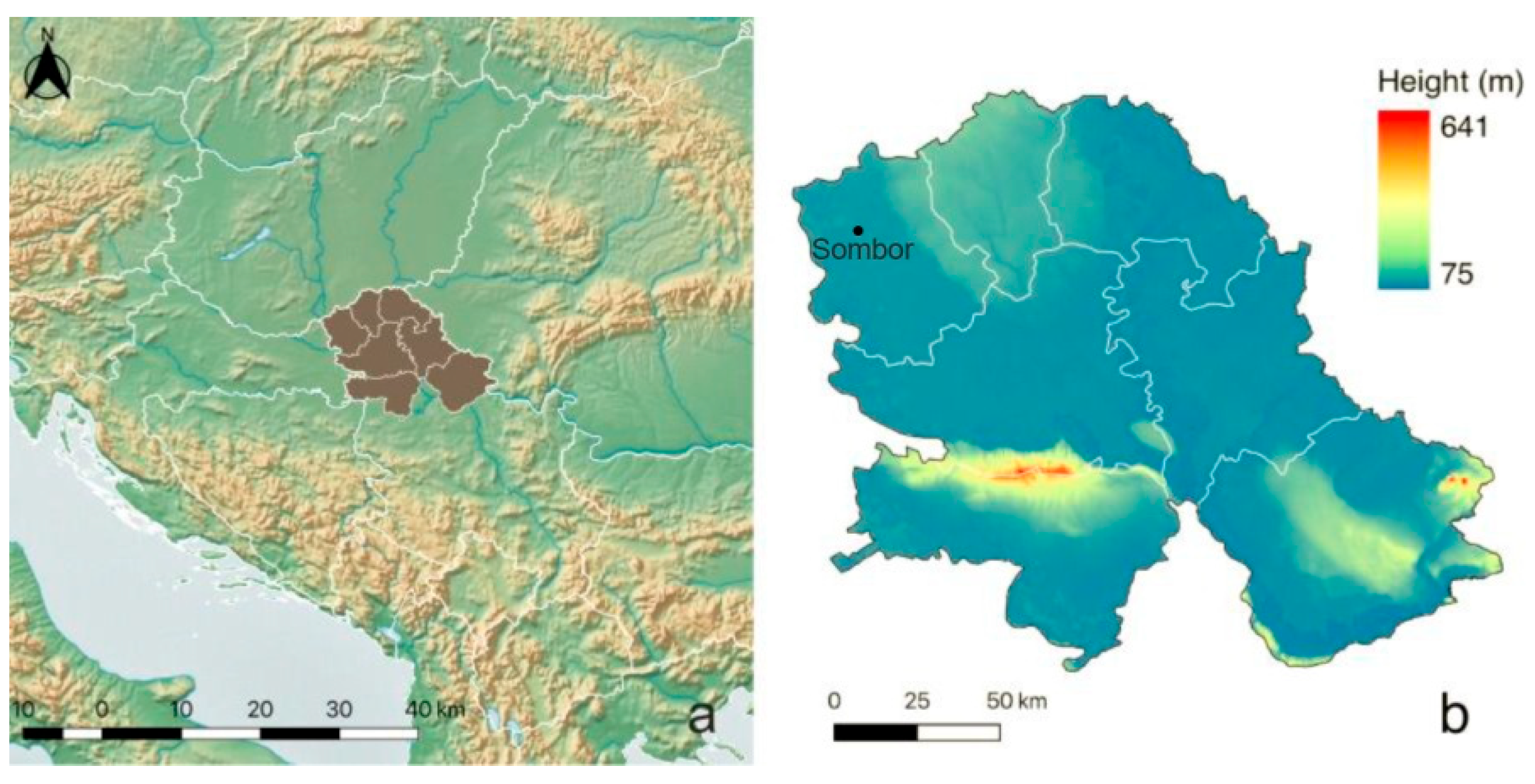
Numerous measurements are available that provide an excellent foundation for studying the complexity of precipitation in relation to various meteorological elements. These data sources range from observations collected by standard meteorological networks to advanced satellite-based measurements such as those from the GPM Dual-frequency Precipitation Radar (DPR) [8]. In this study, we utilized two types of datasets [observed (O) and climate simulation data (M)] for the city of Sombor (45.78° N, 19.12° E) in Vojvodina Province, Serbia (Figure 3a,b).

The analysis covered the period from 1982 to 2005. The observed dataset included monthly values for precipitation (PRE), mean temperature (T_av), minimum and maximum temperatures (T_min and T_max), wind speed (WS), and global radiation (GR), sourced from the Republic Hydrometeorological Institute of Serbia. The climate simulation data were generated using a dynamic downscaling technique with the EBU-POM model under the pessimistic SRES-A2 greenhouse gas emissions scenario. EBU-POM is an atmosphere–ocean regional coupled climate model [9], with horizontal resolutions of 0.25° for the atmospheric component and 0.2° for the oceanic component. The regional model simulations spanned the period 1961–2100, using initial and lateral boundary conditions derived from the ECHAM5/MPI-OM global climate model [10]. All time series were normalized as follows: Given a time series $\begin{array}{cc}\left\{x_i\right\},& i=1,\hspace{0.33em}2,\hspace{0.33em}3,\hspace{0.33em}4,\hspace{0.33em}...,\hspace{0.33em}N\end{array}$, normalization was performed using the transformation, $x_i=(X_i-X_{min})/(X_{max}-X_{min})$, where $\left\{X_i\right\}$ represents the original time series (either observed or simulated), $X_{max}=max\left\{X_i\right\}$ is the maximum value in the series, and $X_{min}=min\left\{X_i\right\}$ is the minimum value. This normalization ensures all values fall within a range of 0 to 1.

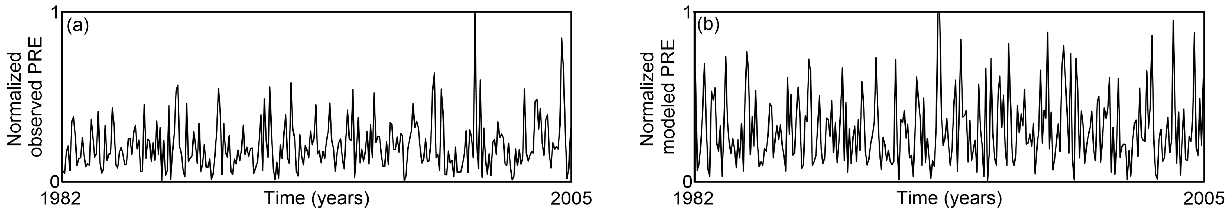
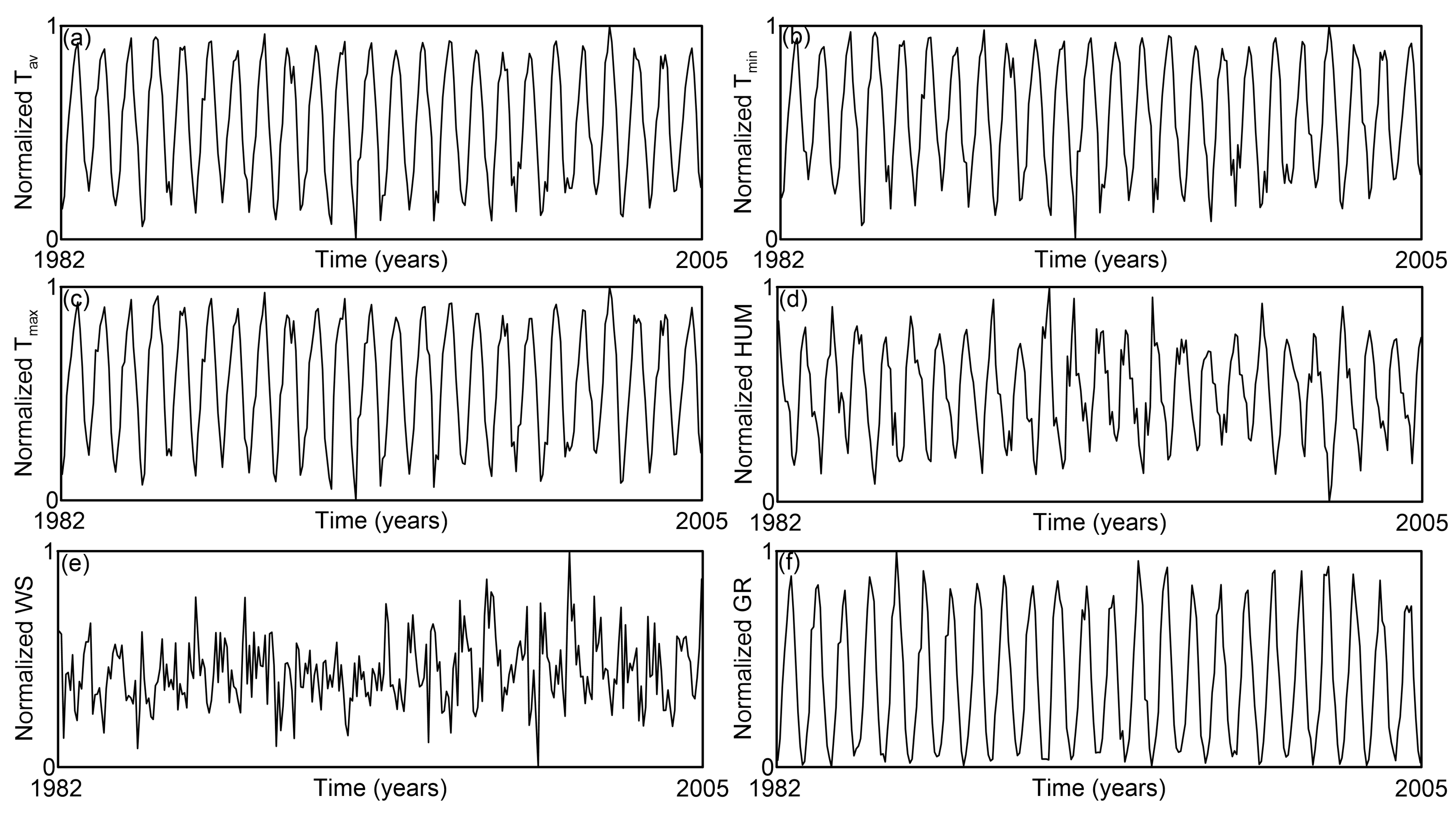
To compare the overall complexity of precipitation with the complexities of individual components (observed and modeled), we employed the normalized time series, which are illustrated in Figure 4, Figure 5 and Figure 6, respectively. Each time series comprised 288 samples.

Table 1. Extremes (maximum and minimum) in meteorological time series.

Variable	Modeled		Observed
	Max	Min	Max	Min
Precipitation (PRE)	156.8 mm	0.0 mm	231.0 mm	0.8 mm
Mean temperature (Tav)	24.5 °C	−5.7 °C	25.0 °C	−6.3 °C
Minimum temperature (Tmin)	16.9 °C	−9.6 °C	16.8 °C	−10.4 °C
Maximum temperature (Tmax)	31.9 °C	−2.7 °C	33.8 °C	−2.3 °C
Humidity (HUM)	86.2%	29.3%	82.4%	29.4%
Wind speed (WS)	3.8 ms−1	1.8 ms−1	2.7 ms−1	1.2 ms−1
Global radiation (GR)	316.9 Wm−2	29.3 Wm−2	325.2 Wm−2	34.2 Wm−2

summarizes the maximum and minimum values used for normalization of the time series data.

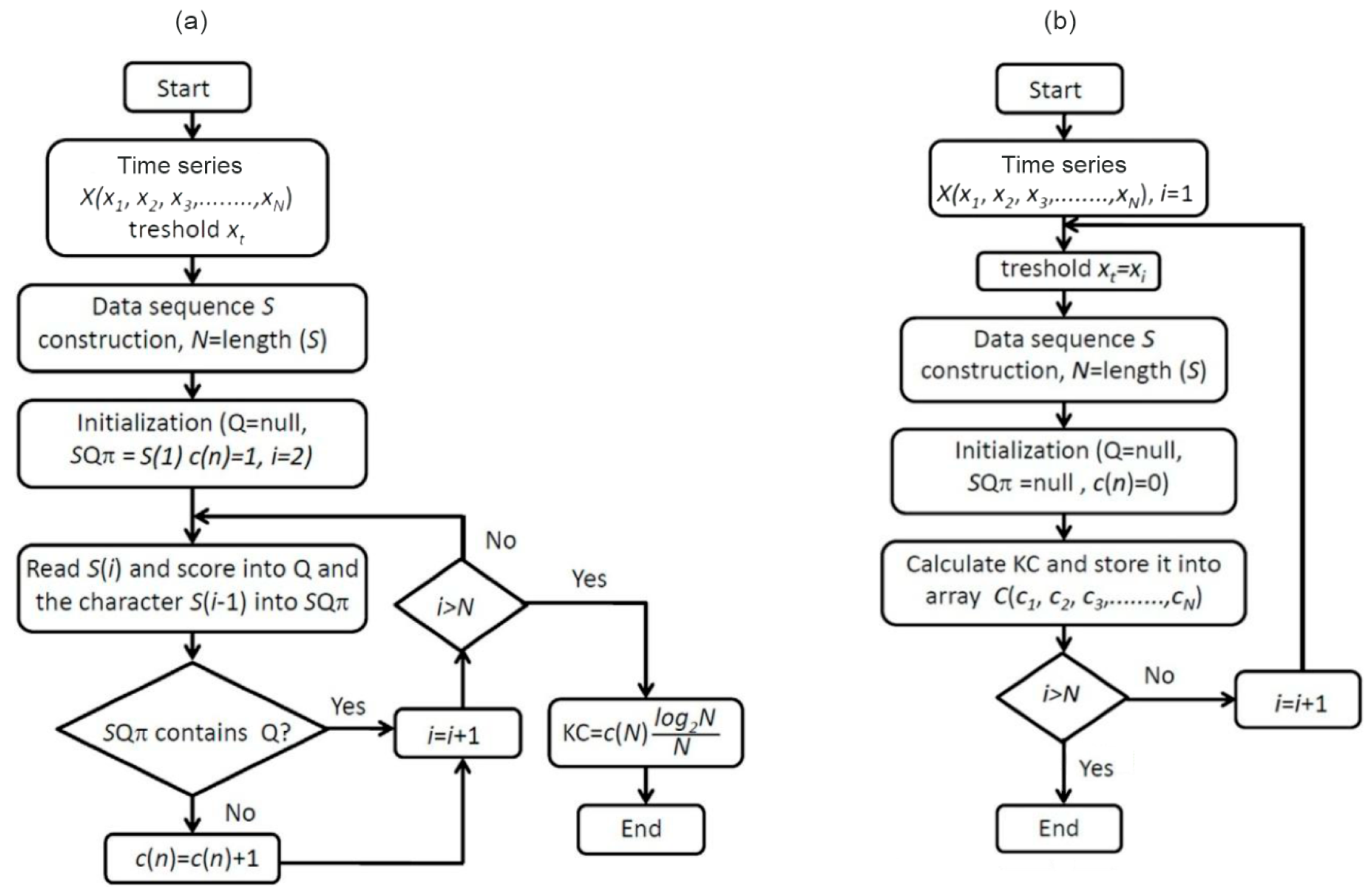
3. Description of Method

We briefly describe a novel method for studying the complexity of precipitation, which involves the following steps: (1) calculation of the Kolmogorov complexity spectrum (KC spectrum) of the quantity of interest, (2) construction of the Kolmogorov complexity plane of interacting amplitudes (KC plane), and (3) computation of the relative change (RC) of the quantity of interest.

(1) Calculation of the KC spectrum of the quantity of interest. Kolmogorov complexity (KC) quantifies the randomness of an object by the length of the shortest program needed to reproduce it (Appendix A). In meteorology, it provides tools to analyze chaotic systems, optimize models, and enhance forecasting accuracy. Kolmogorov complexity (KC) quantifies the degree of randomness and predictability in meteorological time series, including daily or monthly measurements of UV radiation, precipitation, and temperature [11,12,13]. By evaluating the complexity of these datasets, researchers can reveal underlying patterns and dependencies that are often hidden in raw data. This insight enables the development of more effective and accurate models for weather and climate prediction. Specifically, a low Kolmogorov complexity suggests the presence of regular, predictable structures, while a high complexity indicates chaotic dynamics and reduced predictability [14].

Since KC is non-computable for arbitrary objects, it is typically approximated using compression-based methods such as the Lempel–Ziv algorithm (LZA) [15]. Nevertheless, a key limitation of LZA arises from its reliance on binary time series. The binarization preprocessing step required to apply LZA can lead to information loss, as nuances in the original data may not be fully preserved in the binary representation. However, despite some drawbacks, LZA remains widely used due to its adaptivity, simplicity, and asymptotic optimality without requiring prior knowledge of source statistics. Implementations of this algorithm are available in multiple programming languages and can be found readily online.

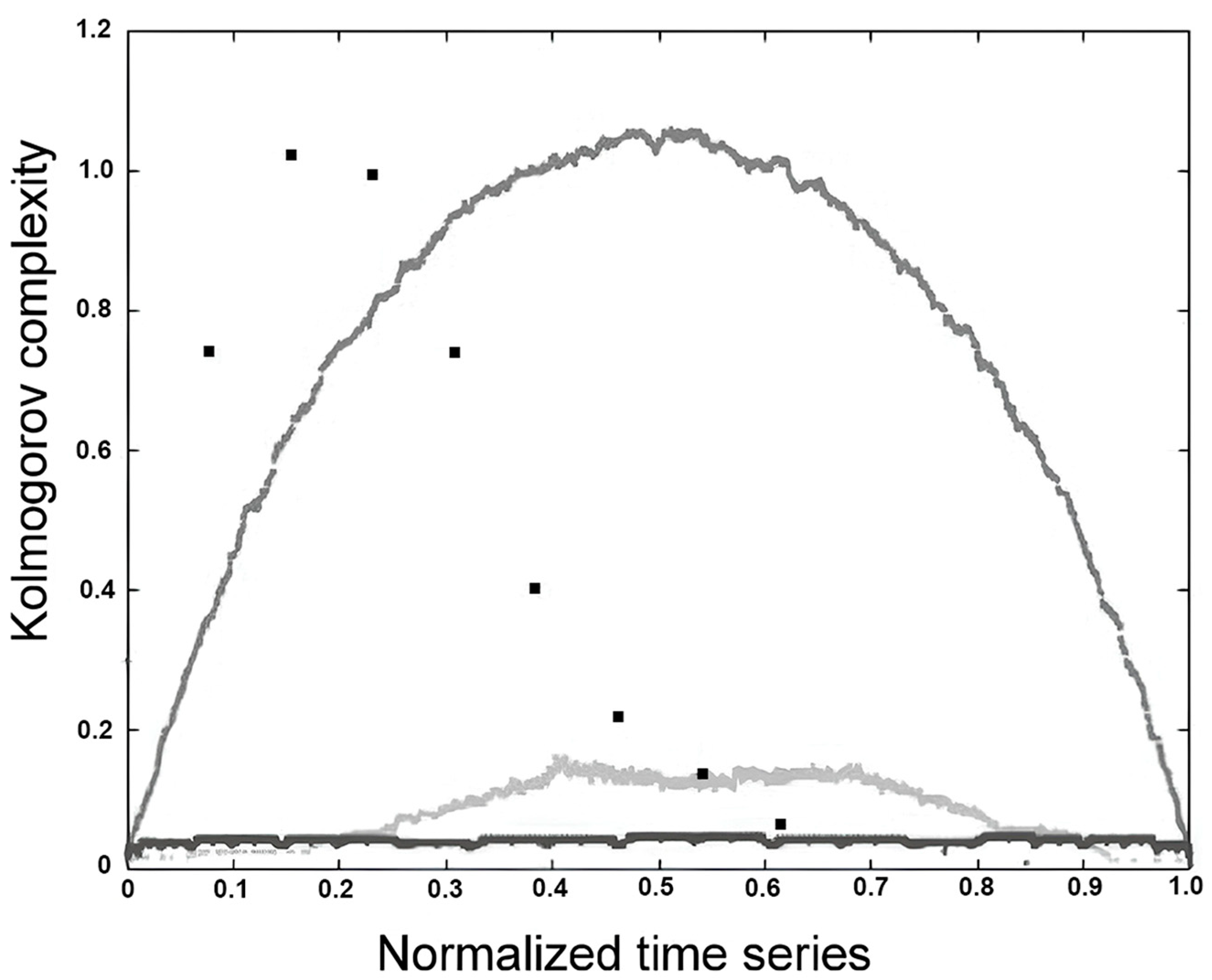
The KC spectrum introduced by Mihailović et al. [16] provides a novel framework for analyzing complex systems characterized by high levels of complexity and stochasticity. Figure 7 illustrates the KC spectra computed for several types of time series: quasi-periodic, Lorenz attractor, random with uniform distribution, and random with Poisson distribution. The figure clearly demonstrates the ability of the KC spectrum to effectively distinguish chaotic and quasi-periodic dynamics from purely random processes, highlighting its sensitivity to underlying structural differences in time series data. Calculating KC spectrum using the LZA is outlined in Appendix A; for a more comprehensive explanation, see Appendix A in Physics of Complex Systems: Discovery in the Age of Gödel [17].

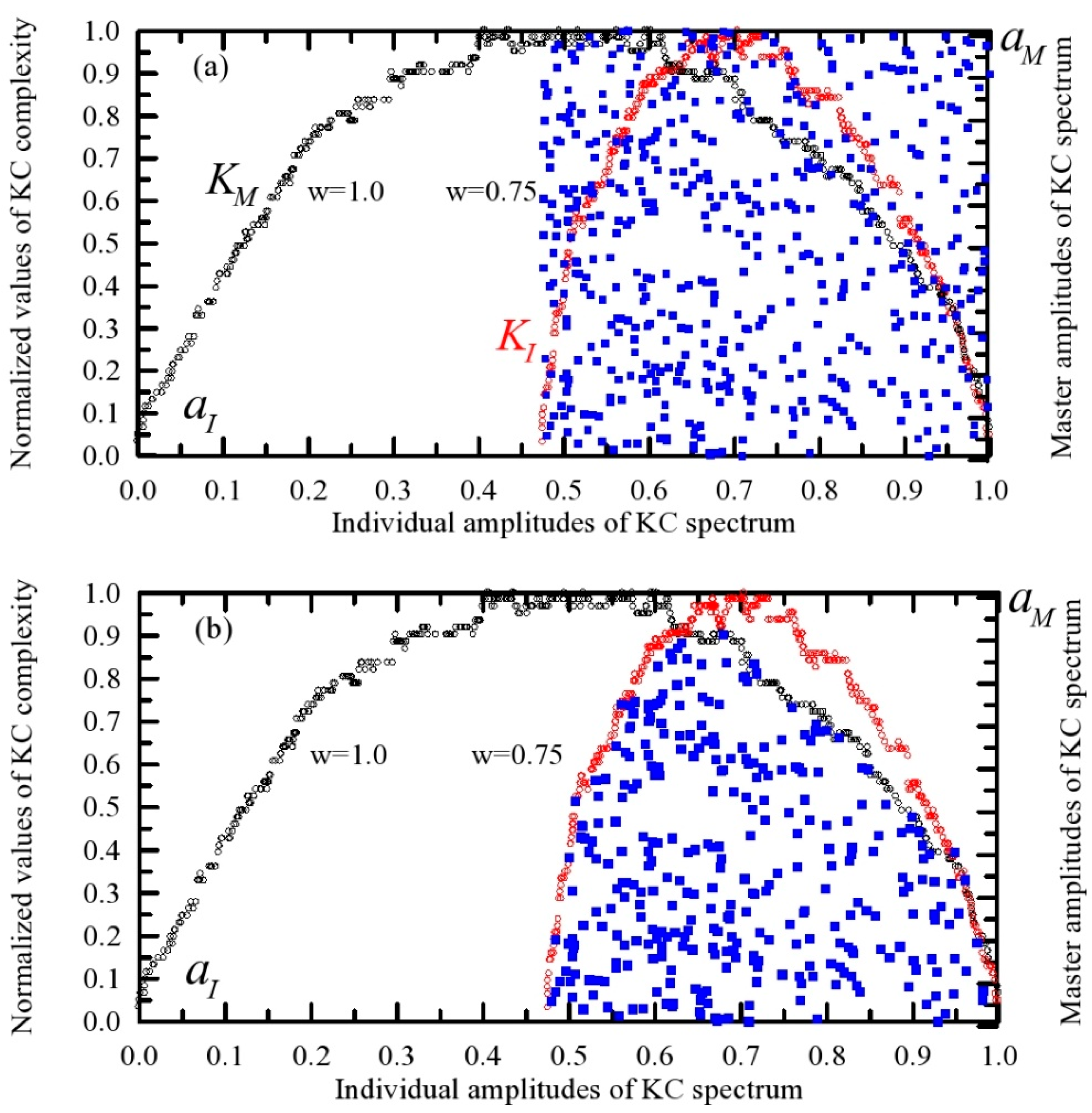
(2) Defining the KC plane in the context of interacting amplitudes. One of the most challenging tasks in studying complex physical systems is determining the contributions of the complexities of individual components to the overall complexity of the entire system. The Kolmogorov complexity plane of interacting amplitudes (KC plane) is a conceptual framework used to analyze the contributions of individual components to the overall complexity of a system. This approach, introduced by Mihailović and Singh [18], employs the KC plane in a two-dimensional space (1,1) to study physical systems and their components through their respective complexities.

To illustrate this concept, we use time series data $\left\{x_{\mathrm{i}}\right\},i=\mathrm{1,2},3,\dots ,N$ generated as $x_i\left\{x_i\right\}=e^{-w{\sigma }_i}$, where $ww$ is the amplitude factor and ${\sigma }_i$ is a random number uniformly distributed over the interval [0, 1]. We generated two time series with $ww=1.0$ and $ww=0.75$, as carried out in [19], corresponding to the master and individual components of the KC spectra $K_M$ (black circles) and $K_I$ (red circles), respectively (Figure 8). In this study, for example, the master component can represent precipitation, while the individual components may include extreme temperatures, mean temperature, wind speed, humidity, and global radiation.

In the coordinate system ($X,Y$), the $X$-coordinate represents the individual amplitude of the KC spectrum ($a_I$), while the $Y$-coordinate corresponds to the normalized value of the KC spectrum ($K_C-\mathrm{K}\mathrm{C}\mathrm{s}\mathrm{p}\mathrm{e}\mathrm{c}\mathrm{t}\mathrm{r}\mathrm{u}\mathrm{m}\mathrm{a}\mathrm{x}\mathrm{i}\mathrm{s})$(as shown in Figure 8). The set of points in this system, depicted as blue squares in Figure 8a, is formed by elements taken from the time series of $K_I$ and $K_M$ and the combined $K_I{K}_M$ spectra, resulting in $N$ points. This representation effectively maps the spectral amplitudes against their normalized values, facilitating analysis of their relationships within the time series data. However, interaction between the master and individual amplitudes exists only at points belonging to the surface bounded by the curves $K_I$ and $K_M$ (Figure 8b). Hence, the name interacting amplitudes. The region bounded by segments of the $K_I$ and $K_M$ spectra and the x-axis (individual amplitude axis) is symbolically designated as the KC plane. The key variables, including precipitation complexity, other meteorological parameters, and spatial patterns at points in the KC plane, can be directly compared using a normalized two-dimensional framework (0–1 scale). By standardizing their time series, all metrics operate on a uniform scale, eliminating distortions caused by differing units or magnitudes. This standardization enables precise evaluation of relationships, patterns, and synergies between variables without scale-related bias [20].

To evaluate points against both discrete curves, we employed nonlinear curve comparison methods available in R packages. For the fitting procedure used to calculate complexities in the $(a_I,a_M)$ system, we replaced the previous approach with cubic spline interpolation, which provides a smoother and more accurate fit, as supported by recent studies on meteorological data modeling [21]. When determining the number of points within the KC plane, a small fraction of points that technically falls outside the defined boundaries are still included in the count. However, in this study, such outlier points constitute less than 0.05% of the total, making their impact on the overall analysis negligible.

(3) Computation of the relative change (RC) of the quantity of interest. To quantify the interrelationship between the complexities of the master and individual components, we employ a simple method consisting of the following steps: (1) Identify the KC plane as the overlapping area (OA) for analysis. (2) For each point in the OA, locate its coordinate on the $a_I$ axis (individual amplitudes axis) and extract the corresponding KC value from the precipitation KC spectrum. (3) Determine the mean KC value within the OA for precipitation (PER) and $T_{av}$ T_av, T_min, T_max, HUM, WS, and GR as individual components. (4) Compute the relative change [RC = (B − A)/A × 100)] from quantity A to quantity B, where A is an initial value (PER) and B is a final value ($T_{av}$ T_av, T_min, T_max, HUM, WS, and GR).

The threshold of minimal change in KC indicates a shift in the complex systems (TKC). Our analysis of the relationship between overall complexity and individual complexities will be grounded in Kolmogorov complexity (KC) analyses, such as Lempel–Ziv complexity, within the set. This raises the question of what thresholds of minimal change (TKC) in KC signify a shift in complex systems. While there is no universal minimal KC threshold, relative changes reliably indicate systemic shifts in complex systems. Let us examine some practical threshold values derived from various studies. In cardiology, atrial fibrillation is associated with highly complex local electrical activity, as reflected in the rich morphology of intracardiac electrograms [22]. In this context, the authors used a TKC of 5%. For fluid dynamics, a change greater than 10% in the vertical distribution of KC or its spectrum can indicate a transition from steady to unsteady flow conditions, such as during the passage of an undular surge [23]. In meteorology, detecting minimal changes in KC that indicate significant shifts in complex systems—like weather patterns or climate dynamics—requires analyzing the KC spectrum. Changes in the smoothness or peak distribution of the KC spectrum can signal shifts in weather patterns. For example, low values may disrupt the spectrum’s smoothness, reflecting increased complexity under certain conditions (e.g., partly cloudy conditions affecting solar radiation variability) when TKC exceeds 10% [11]. Kovalsky et al. [24] analyzed outputs from LIGO experiments—which fall under gravitational physics, specifically focusing on general relativity and gravitational wave astronomy—using KC spectra of residual, raw, and template time series from the Hanford and Livingston observatories. Their analysis revealed valuable insights regarding the interval (0.02, 0.18) of KC, providing critical context for interpreting gravitational wave detection methodologies.

We believe it is essential, within the Methods Section, to present the facts concerning the threshold of minimal change in Kolmogorov complexity (KC) that signals a shift in complex systems. Firstly, it is quite rare across many scientific disciplines to compile empirical evidence regarding KC thresholds at which system dynamics undergo significant changes. Secondly, in this study focused on a physical complex system, identifying these thresholds is crucial for analyzing the complexity and interdependencies among climatic elements.

4. Results and Discussion

Initially, we will discuss the rationale behind selecting the aforementioned meteorological variables to analyze the complexity of precipitation. Temperature (mean/maximum minimum) directly influences atmospheric moisture content, determining the precipitation intensity and variability (thermodynamic effects). Temperature gradients influence atmospheric circulation patterns, which in turn affect vertical motion and precipitation formation processes (dynamic effects). Atmospheric humidity is a critical factor in precipitation potential. As humidity increases, it enhances convective stability, thereby elevating the risk of extreme precipitation events. Wind speed is essential for transporting moisture and affecting convergence zones, where the conditions are favorable for precipitation to form. Solar radiation is a key driver of surface heating, which in turn affects evaporation rates and atmospheric instability. Changes in solar radiation also have a profound impact on cloud microphysics and boundary layer dynamics, contributing to complex weather phenomena. These meteorological variables collectively represent both thermodynamic (e.g., moisture availability) and dynamic (e.g., atmospheric motion) processes that govern the complexity of participation. While factors such as vertical velocity or specific weather systems could refine understanding, this framework provides a robust foundation for analyzing precipitation dynamics.

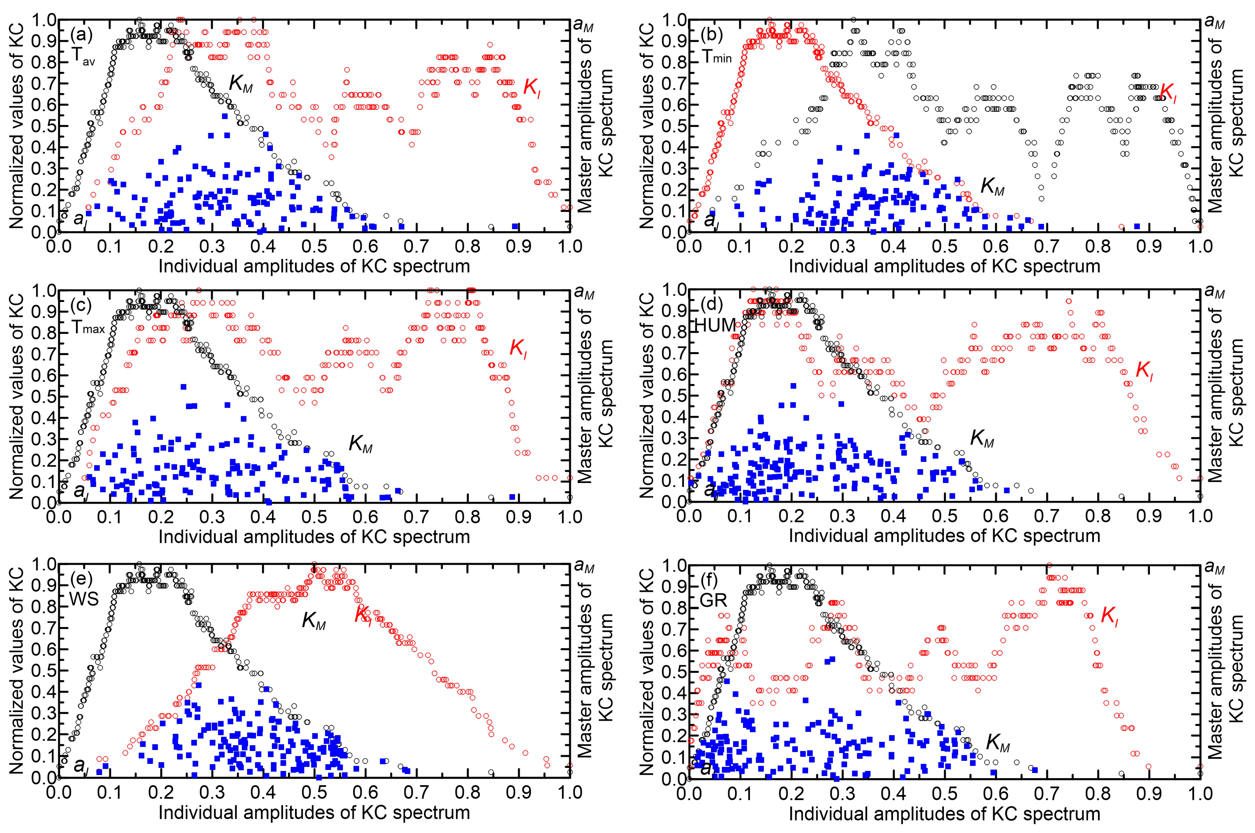
The complexity of precipitation has been extensively studied in both historical and contemporary research [7,25,26,27]. Despite the breadth of these studies, most primarily employ entropy-based information measures and conventional statistical techniques. A key gap remains in explicitly quantifying how the overall complexity of precipitation systems (the master complexity) relates to the complexities of their constituent components (the individual complexities) within the overlapping area (OA). In this study, these components specifically include mean temperature, minimum and maximum temperatures, humidity, wind speed, and global radiation. In Figure 9 and Figure 10, points of interacting amplitudes are visually represented by blue squares.

The results from steps (1)–(3) are detailed in

Table 2. Statistics with observed data for Sombor (Serbia). Gray highlighted numbers represent maxima in each column.

Normalized Individual Amplitude	Values of KC in the Overlapping Area (OA) and (Number of Points in OA)
	Tav	Tmin	Tmax	HUM	WS	GR
0.0–0.1	0.756 (2)	0.756 (2)	0.817 (7)	0.620 (27)	0.295 (2)	0.694 (45)
0.1–0.2	0.704 (19)	0.734 (8)	0.614 (31)	0.688 (61)	0.795 (4)	0.684 (26)
0.2–0.3	0.646 (37)	0.621 (29)	0.722 (32)	0.738 (31)	0.725 (23)	0.640 (30)
0.3–0.4	0.687 (32)	0.677 (38)	0.698 (39)	0.773 (28)	0.749 (50)	0.766 (21)
0.4–0.5	0.722 (24)	0.768 (32)	0.698 (17)	0.748 (17)	0.692 (43)	0.691 (21)
0.5–0.6	0.627 (11)	0.662 (11)	0.673 (16)	0.701 (9)	0.710 (33)	0.777 (13)
0.6–0.7	0.179 (3)	0.292 (5)	0.256 (3)	0.410 (1)	0.325 (3)	0.282 (1)
0.7–0.8
0.8–0.9	0.179 (1)	0.179 (1)	0.179 (1)
0.9–1.0
Average (sum)	0.665 (129)	0.672 (126)	0.674 (136)	0.705 (174)	0.709 (158)	0.696 (157)

and

Table 3. Statistics with EBU-POM output data for Sombor (Serbia). Gray highlighted numbers represent maxima in each row.

Normalized Individual Amplitudes	Values of KC in the Overlapping Area (OA) and (Number of Points in OA)
	Tav	Tmin	Tmax	HUM	WS	GR
0.0–0.1	0.772 (6)	0.693(3)	0.772 (3)			0.756 (31)
0.1–0.2	0.734 (20)	0.727 (19)	0.741 (23)	0.583 (12)	0.546 (8)	0.711 (37)
0.2–0.3	0.745 (38)	0.786 (29)	0.758 (39)	0.769 (35)	0.774 (36)	0.763 (31)
0.3–0.4	0.740 (34)	0.737 (34)	0.762 (24)	0.647 (37)	0.721 (60)	0.908 (10)
0.4–0.5	0.778 (22)	0.742 (30)	0.788 (24)	0.721 (33)	0.723 (68)	0.744 (23)
0.5–0.6	0.757 (23)	0.728 (23)	0.751 (20)	0.811 (35)	0.813 (40)	0.687 (11)
0.6–0.7	0.679 (10)	0.719 (13)	0.726 (12)	0.754 (39)	0.778 (20)	0.713 (19)
0.7–0.8	0.613 (14)	0.668 (16)	0.616 (15)	0.668 (18)	0.737 (3)	0.626 (13)
0.8–0.9	0.237 (5)	0.417 (6)	0.312 (7)	0.579 (2)		0.303 (2)
0.9–1.0	0.377 (3)	0.281 (3)	0.322 (4)			0.184 (1)
Average (sum)	0.714 (175)	0.717 (176)	0.717(171)	0.723 (211)	0.744 (235)	0.728 (178)

. The KC values, which are quantified, are 0.677 for the observed data and 0.697 for the EBU-POM output time series. Inspection reveals that the highest KC values for both observed and modeled time series are generally located in the left half of the normalized individual amplitude, i.e., the interval (0,1), except for the GR component in the observed time series and the HUMand WS components in the modeled time series. Notably, the observed time series shows its highest maxima value (0.817) in the 0.0–0.1 interval for the T_max component, with the lowest maxima value (0.756) in the 0.0–0.1 interval for the T_av component. Conversely, the modeled time series exhibits its highest maxima KC value (0.908) in the 0.3–0.4 interval for the GR component, while the lowest maxima KC value (0.778) is found in the 0.4–0.5 interval for the T_av component.

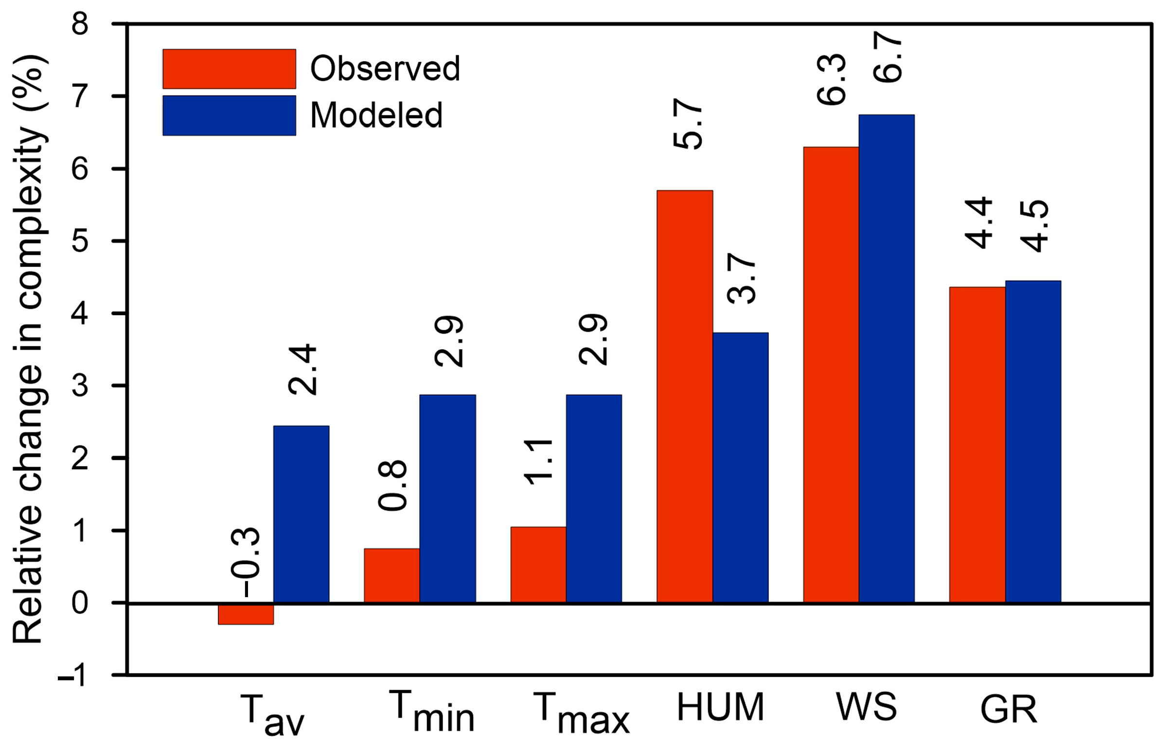
Figure 11 can be interpreted as follows: Component contributions in observed data. Wind speed (RC = 6.3%) and humidity (RC = 5.7%) dominate as the most complex components, indicating their roles as primary drivers of unpredictability in precipitation dynamics. Wind speed governs turbulence and atmospheric transport, while humidity directly affects moisture availability and cloud formation [28,29]. Temperature extremes (minimum RC = 0.8%; maximum RC = 1.1%) slightly exceed the mean temperature (RC = –0.3%), suggesting daily temperature fluctuations are more influential than average conditions in shaping precipitation variability. Global radiation (RC = 4.4%) closely aligns with precipitation’s complexity, highlighting its role in energy balance and evaporation processes [28]. Overall vs. component complexity. The system’s overall complexity (KC = 0.667) is lower than T_min, T_max, WS, HUM, and GR (see averaged values in Table 2), implying that interactions between variables introduce partial regularity, slightly reducing the system’s total randomness. No single component fully dictates the system’s behavior; instead, their combined effects create emergent complexity [28,30]. Modeling challenges. High complexity in WS, GR, and HUM suggests that these variables require advanced nonlinear models or machine learning to capture their chaotic dynamics. This analysis highlights the need to prioritize wind speed, humidity, and radiation in precipitation modeling while accounting for their nonlinear interactions.

Figure 11 reveals that the histograms for both observed and modeled time series exhibit similar shapes, indicating that the analysis conducted on observed values is also applicable to modeled values. However, the relative changes are generally higher in the modeled series compared to the observed ones, except for humidity. The reason for these differences in relative changes in complexity stems from the fact that the mean KC values for component systems in the modeled time series are systematically larger than those in the measured series (see mean KC values in Table 2 and Table 3). Namely, climate models typically display higher KC in variable simulations compared to measured data, primarily due to inherent design factors and the intrinsic chaotic nature of climate systems. The following are key reasons contributing to this phenomenon: chaotic dynamics and nonlinear interactions, temporal and spatial resolution, structural differences in data representation, and model-specific amplification.

Figure 11 contains information that, to the author’s knowledge, has not been available before, i.e., the values of relative changes (RC) of complexity for individual components (mean temperature, minimum temperature, maximum temperature, humidity, wind speed, and global radiation) in relation to the overall complexity of precipitation. These values can be either positive or negative. A positive relative change in the complexity of precipitation compared to the complexity of a meteorological element indicates that the variability or intricacy of precipitation patterns increases relative to the variability or intricacy of the meteorological element patterns. Otherwise, the variability or intricacy of precipitation patterns decreases relative to the variability or intricacy of the meteorological element patterns. When examining the values, it is evident that the highest impact on the overall complexity of precipitation comes from wind speed (6.7%), humidity (5.7%), and global radiation (4.4%) for observed values, and similarly for modeled values. In terms of overall complexity, humidity and temperature are generally considered the most influential factors due to their direct roles in moisture availability and atmospheric stability [31,32,33]. Wind speed plays a significant role in shaping precipitation patterns through moisture transport and convergence [34]. Global radiation has a more indirect influence but is essential for driving the atmospheric processes that lead to precipitation. This order reflects the directness and magnitude of their impact on precipitation processes. However, the specific influence of each factor can vary depending on geographical location and specific weather conditions. It can be observed in our example that all meteorological elements that most influence the complexity of precipitation are listed, except for temperature, which, due to geographical factors, has a negative relative change in complexity in relation to the complexity of precipitation (–0.2%). This negative relationship may reflect a suppression of precipitation dynamics as temperatures rise, which can occur due to several climatic and physical factors [35].

When the relative change in the overall complexity of precipitation is less than the individual complexities contributed by humidity (5.7%), wind speed (6.3%), and global radiation (4.4%), it suggests that precipitation patterns are less variable or less dynamically complex over time compared to these other meteorological variables. This can imply several things in the context of climate or weather system analysis: (1) Precipitation dynamics may be more stable or less sensitive to changes in environmental conditions relative to humidity, temperature, and wind speed, which show greater complexity changes. (2) The processes controlling precipitation might be governed by more constrained or deterministic mechanisms, whereas humidity, temperature, and wind speed could be influenced by more diverse or chaotic factors, leading to higher complexity changes. (3) Lower relative complexity change in precipitation could indicate that precipitation variability is less responsive to climate variability or that it integrates multiple atmospheric factors, smoothing out complexity fluctuations seen in individual variables like temperature or wind. (4) From a predictability standpoint, precipitation might be comparatively more predictable or less prone to abrupt changes than the other variables if its complexity changes less [8]. Finally, the differential complexity changes reflect the reorganization of climate subsystem interactions, which is consistent with studies showing that KC variations >2–3% can induce measurable regime shifts in environmental systems. The largest impacts likely stem from wind and radiation changes, which mediate energy/mass exchanges critical to regional climate stability.

At the end of the Results and Discussion Section, we will provide explanations based on some of the reviewers’ questions. Their feedback was strong but constructive, focusing on the potential applications of this novel method in atmospheric sciences. In particular, they emphasized the need to explain the method in simple terms for audiences unfamiliar with complexity spectrum theory; clarify how the results provide new insights into the precipitation process; discuss the potential limitations and the conditions under which the method is applicable; and highlight why this research is important while outlining future plans.

In this study, an effort was made to present a proposed information measure as simply as possible through flowcharts and code available online in different programming languages.

The method suggested enriches precipitation research by providing a robust measure of randomness and complexity beyond traditional entropy-based metrics, detecting multiscale interactions and transitions in precipitation processes, and offering insights into the influence of environmental changes on precipitation dynamics.

Although this method offers a powerful framework for analyzing the complexity of precipitation time series, it has some potential limitations. It requires high-quality, high-resolution data and is most effective in contexts where nonlinear interactions play a significant role. Additionally, its interpretation is significantly enhanced when complemented by a solid physical understanding of the underlying precipitation processes.

This research essentially focuses on one key aspect: the quantification of the complexity of components within a complex physical system, such as precipitation. It reveals relative changes in overall complexity compared to the complexity of individual system components—patterns that cannot be detected using traditional mathematics and statistics. After establishing the method, the next step would be to test it on long-term, high-resolution, and high-quality precipitation time series data. It is important to note that relying solely on monthly data may limit Kolmogorov complexity’s ability to detect nonlinear interactions present at daily or hourly scales, as temporal aggregation tends to smooth out high-frequency variability. However, the magnitude of this limitation depends on the data processing techniques and the inherent characteristics of the underlying variability. Therefore, the next step should involve testing the proposed method on long-term, high-resolution, and high-quality precipitation time series data to ensure robustness and accuracy.

5. Conclusions

This study analyzed how the complexity of individual components (mean temperature, temperature extremes, humidity, wind speed, and global radiation) influences the overall or master complexity of both observed and modeled precipitation.

We selected six time series, including the monthly data simulated by the EBU-POM regional climate model for the 1982–2005 period (Sombor, Serbia), as well as the measured monthly time series of mean temperature and temperature extremes, humidity, wind speed, and global radiation averaged over the same period.

The Kolmogorov complexity spectrum (KC spectrum) and Kolmogorov complexity plane (KC plane) were effective in quantifying the complexities of precipitation and its meteorological components.

This study demonstrates that the overall complexity of precipitation arises from the combined complexities of its individual components. By examining overlapping regions within the KC spectra, specific coordinates in the KC plane can be identified; at these coordinates, KC values are calculated using data derived from the individual amplitude axes.

We proposed a simplified four-step method to compute the relative change in complexities within the overlapping area beneath the KC spectra.

This study introduced a novel framework that links meteorological variables to emergent patterns in precipitation complexity, offering insights beyond those of existing methods.