Article

Ensemble Learning-Based Soft Computing Approach for Future Precipitation Analysis

by
Shiu-Shin Lin
1,*,
Kai-Yang Zhu
1,
Chen-Yu Wang
1,
Chou-Ping Yang
2 and
Ming-Yi Liu
1
1
Department of Civil Engineering, Chung Yuan Christian University, Taoyuan City 320314, Taiwan
2
Graduate Institute of Landscape Architecture and Recreation Management, National Pingtung University of Science and Technology, Pingtung 912301, Taiwan
*
Author to whom correspondence should be addressed.
Atmosphere 2025, 16(6), 669; https://doi.org/10.3390/atmos16060669
Submission received: 31 March 2025 / Revised: 12 May 2025 / Accepted: 27 May 2025 / Published: 1 June 2025
(This article belongs to the Special Issue The Hydrologic Cycle in a Changing Climate (2nd Edition))

Abstract

:
This study integrated the strengths of ensemble learning and soft computing to develop a future regional rainfall model for evaluating the complex characteristics of island precipitation. Soft computing uses the well-developed adaptive neuro-fuzzy inference system, which has been successfully applied in atmospheric hydrology and combines the features of neural networks and fuzzy logic. This combination enables artificial intelligence (AI) to effectively represent reasoning derived from complex data and expert experience. Due to the multiple atmospheric and hydrological factors that influence rainfall, the nonlinear interrelations among them are highly intricate. Nonlinear principal component analysis can extract nonlinear features from the data, reduce dimensionality, and minimize the adverse effects of data noise and excessive input factors on soft computing, which may otherwise result in poor model performance. Ultimately, ensemble learning enhances prediction accuracy and reduces uncertainty. This study used Tamsui and Kaohsiung in Taiwan as case study locations. Historical monthly rainfall data (January 1950 to December 2005) from Tamsui Station and Kaohsiung Station of the Central Weather Administration, along with historical and varied emission scenario data (RCP 4.5 and RCP 8.5) from three AR5 GCM models (ACCESS 1.0, CSIRO-MK3.6.0, MRI-CGCM3), were used to evaluate future regional rainfall trends and uncertainties through the method proposed in this study. The research findings indicate the following: (1) Ensemble learning results demonstrate that all examined general circulation models effectively simulate historical rainfall trends. (2) The average rainfall trends under the RCP 4.5 emission scenario are generally consistent with historical rainfall trends. (3) The exceedance probabilities of future rainfall during the mid-term (2061–2080) and long-term (2081–2100) suggest that Kaohsiung may experience precipitation events with higher rainfall than historical data during dry seasons (October to April of next year), while Tamsui Station may exhibit greater variability in terms of exceedance probabilities. (4) Under both the RCP 4.5 and RCP 8.5 emission scenarios, the percentage changes in future rainfall variability at Kaohsiung Station during dry seasons are higher than those during wet seasons (May to September), indicating an increased risk of extreme precipitation events during dry seasons.

1. Introduction

Precipitation is a vital source of regional water resources. Prolonged rainfall shortages may lead to water scarcity and drought, while short bursts of intense rainfall may cause flooding, posing challenges to the utilization and management of water resources [1]. Climate warming directly impacts the global atmospheric and hydrological environment, placing water resources at the forefront. Consequently, it imposes direct and indirect threats on the daily lives of humans, the economy, and other aspects. Therefore, evaluating the impacts of climate change on water resources has been a focus of relevant researchers, and understanding future climatic change impacts on rainfall trends, characteristics, and uncertainties has emerged as a critical area of scientific study [2]. Currently, most predictions on potential climate changes rely on results from general circulation models (GCMs) as a foundational reference for further application [3]. However, the coarse spatial resolution of GCM data, which typically ranges from tens to hundreds of kilometers horizontally and includes multiple vertical layers from the surface to the upper atmosphere, is inadequate for regional climatic applications. Since the spatial scale of GCM data is too coarse to capture local climatic features, downscaling techniques are employed to refine spatial resolution, thereby facilitating the exploration of regional climate characteristics [4,5,6,7]. In addition to spatial scale limitations, regional climatic characteristics are often influenced by interactions between regional climate and geographical features. For instance, Taiwan, situated at the intersection of the West Pacific and the Eurasian continent, has complex topography [1] and diverse climatic features, making the estimation of precipitation pattern changes induced by climate change and future rainfall even more challenging.
Statistical downscaling is commonly used to apply GCM data for regional climate estimation. Its core concept involves establishing statistical relationships based on long-term observation data and climate model simulation data, which are then used for future climate model estimation data to predict future regional climate conditions [8]. Over the past 20 years, statistical downscaling has evolved beyond traditional statistical methods with the advancement of artificial intelligence (AI)-related technologies, such as soft computing (SC) and machine learning (ML) [7,9]. The adaptive neuro-fuzzy inference system (ANFIS), a method within SC, integrates the advantages of neural networks (NN) and fuzzy logic (FC), enabling it to simulate expert decision-making processes and effectively address nonlinear and ambiguous reasoning problems [9,10]. It is frequently applied across various fields for reasoning and decision-making tasks [11,12] and has been extensively utilized in evaluating Taiwan’s water resources and rainfall estimation. These applications demonstrate that ANFIS is suitable for regional water resource evaluations [9,10]. Enhancing statistical downscaling methods with the advantages of ANFIS can further improve the reliability of regional climate and rainfall trend predictions.
Although ANFIS effectively handles nonlinear data and offers strong model extensibility and interpretability, its prediction accuracy and complexity are significantly influenced by its structure (e.g., the form of membership functions (MFs)) and the characteristics of input data. An excessive number of input variables may lead to a complex model structure, increasing the risk of overfitting and reducing prediction performance [13,14,15,16]. The presence of noise in ANFIS input data may significantly diminish model reliability, often going unnoticed and diminishing its applicability. Implementing feature extraction methods to preprocess raw, complex data can effectively reduce dimensionality and extract nonlinear features, thereby addressing these challenges. Nonlinear principal component analysis (NLPCA) is a widely recognized nonlinear feature extraction technique that differs from traditional principal component analysis (PCA). NLPCA effectively extracts nonlinear principal components (i.e., the nonlinear features of data) from complex datasets, reducing nonlinear dimensionality while simultaneously removing noise [17]. This process enhances the reliability and accuracy of ANFIS.
Besides the challenges related to ANFIS model structure and input variables, few studies have considered the impact of uncertainties in models and data arising from the training, validation, and test datasets used in model construction and their association with the ANFIS model. Research indicates that EL effectively addresses the interactive influences between data and models and establishes the features of data and models with a minimal model. The primary concepts of EL can be categorized into boosting [18], stacking [19], and bagging [20]. The core concept of bagging involves averaging multiple predicted outcomes (regression) or majority voting (classification) to reduce model error and enhance generalization capability. It has been widely applied in weather and climate predictions to reduce forecast uncertainty (unpredictable or probabilistic events) [21,22].
In summary, this study proposes an ANFIS-based downscaling model (BADM) that utilizes NLPCA for nonlinear feature extraction with ANFIS architecture as its core. By employing an improved EL algorithm with the bagging concept, an EL-based ANFIS downscaling model (ELADM) is established based on the BADM framework. By integrating the advantages of nonlinear feature extraction, SC, and EL, the reliability and generalization capability of future regional rainfall estimations are significantly improved. This study used Tamsui and Kaohsiung in Taiwan as case studies to analyze future rainfall differences between northern and southern Taiwan. Using historical monthly rainfall data from Tamsui Station and Kaohsiung Station, as well as GCM models under different scenarios (RCP 4.5, RCP 8.5), the ELADM model is developed to evaluate future rainfall trends and uncertainties for these regions.

2. Materials and Methods

2.1. Nonlinear Principal Component Analysis (NLPCA)

NLPCA is a nonlinear extension of PCA, particularly suitable for data with nonlinear relationships. PCA assumes that data are distributed in a linear space, whereas NLPCA employs NN to capture nonlinear structures within the data, allowing for better information retention during dimensionality reduction. As illustrated in Figure 1, this architecture belongs to a feedforward neural network, where the input layer receives n-dimensional raw data, and the output layer attempts to reconstruct data similar to the original input. The training objective of the NN is to minimize the objective function J. When the mean square error (MSE) of the objective function no longer varies with training iterations, it indicates model convergence. The objective function is presented in Equation (1), where x n and x ^ k represent the nth input and output, respectively; J is the mean squared error over all training samples.
Min   J = x ^ k x n 2
Three hidden layers exist between the input and output layers: the encoding layer, the bottleneck layer, and the decoding layer [23]. The encoding layer compresses the input data ( x n ) via the extraction function ϕ and maps it to the low-dimensional bottleneck layer (p), where neurons are represented as m k (k < n), as shown in Equation (2).
p = ϕ m k
With the least number of NN nodes, the bottleneck layer represents the nonlinear principal components after data dimensionality reduction and is denoted as p. The decoding layer is typically a mirror of the encoding layer. It employs the reconstruction function ψ to restore p to the original data, with neurons represented as m ^ k (k < n), as shown in Equation (3). To ensure effective reconstruction, the entire network adjusts all weights w i during training based on reconstruction errors. In NLPCA, weights facilitate nonlinear mapping from high-dimensional space to low-dimensional space while playing a crucial role in minimizing reconstruction errors and effectively extracting the most significant nonlinear features from the data.
m ^ k = ψ p
The extraction function and the reconstruction function serve as activation functions in NN. Common activation functions include the Smooth Curve Function, the Hyperbolic Tangent Function, and the Gaussian Function. In this study, both the extraction and the reconstruction functions are implemented using the Hyperbolic Tangent Function.
To mitigate the potential overfitting issue caused by excessive noise in input data, Hsieh proposed incorporating a penalty term in the activation function and adjusting it appropriately for resolution [24]. Additionally, to assess the impact of the penalty term and neuron count k on the model, Hsieh integrated MSE with the coefficient of correlation (CC) into a new evaluation indicator, Holistic Information Criteria (HIC) [25], as shown in Equation (4). A lower HIC value indicates better NN performance.
HIC = MSE   ( 1 CC )

2.2. Adaptive Neuro-Fuzzy Inference System (ANFIS)

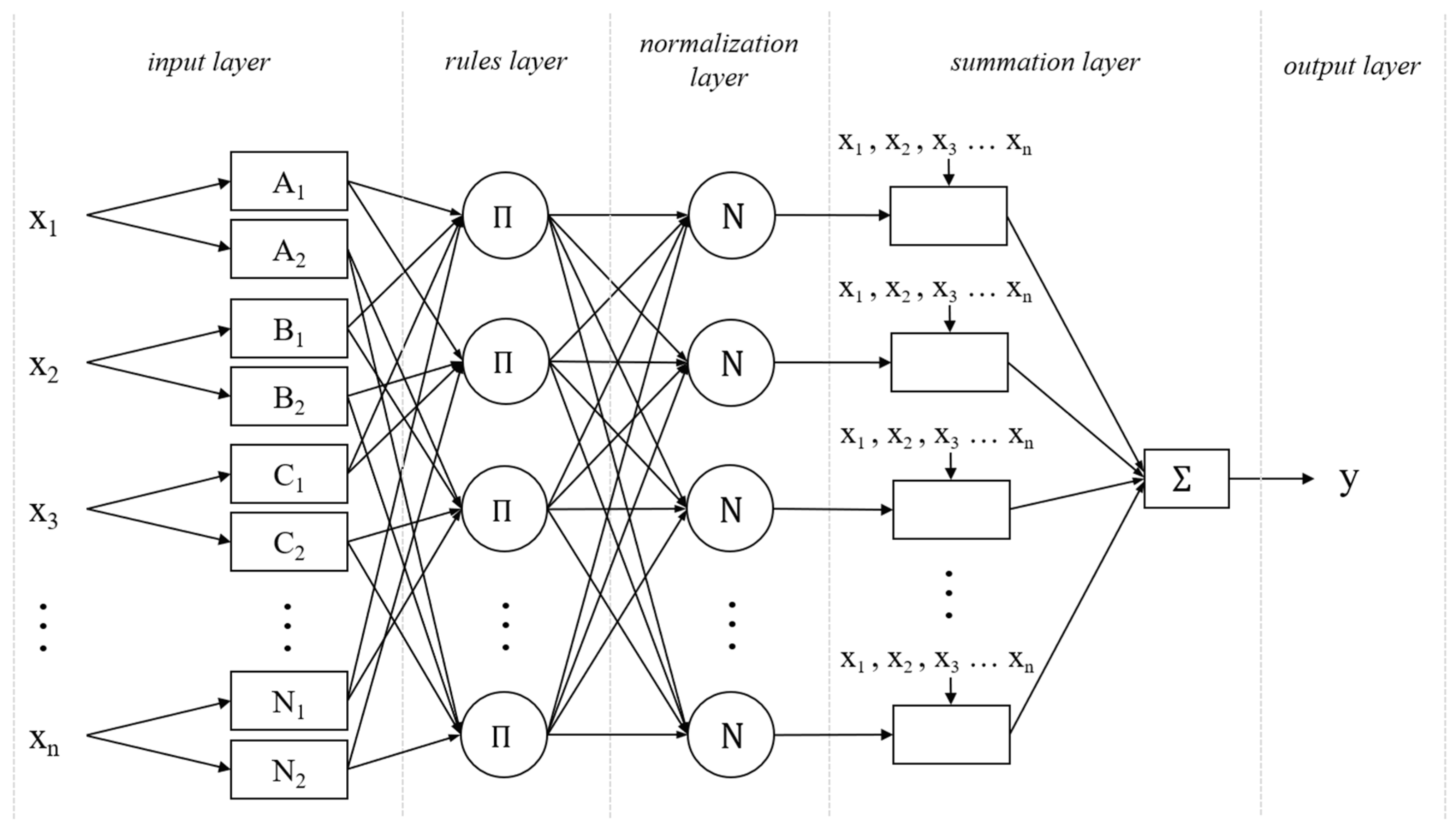
ANFIS is a feedforward neural network that integrates artificial neural networks and fuzzy rules, enabling self-learning and fuzzy reasoning. By leveraging the learning ability of NN and the interpretability of fuzzy logic, it is frequently used to address problems involving uncertainty and ambiguity [16]. In fuzzy logic and inference, the Sugeno fuzzy model is adopted, and similarity functions, such as the Bell function, are constructed for the membership functions (MFs) of nodes at the same layer [26]. By incorporating a feedforward neural network with supervised learning methods, the model parameters can be adaptively adjusted. Parameters within the ANFIS model are categorized into antecedent parameters, which control the shapes of fuzzy functions (e.g., the centers, widths, and curvature parameters of MFs), and consequent parameters, which describe the outputs of fuzzy rules (e.g., linear function coefficients of the Sugeno fuzzy model). As illustrated in Figure 2, the structure of ANFIS is composed of five layers.
(1)
Input layer
The input layer maps input variables to fuzzy sets through MFs. In Figure 2, subsets N1 and N2 belong to the fuzzy set of xn. The transformation equation for the input layer is presented in Equation (5), where μ j x i represents the MFs of the jth set of the ith input variable and a j i , b j i , c j i constitute the antecedent parameters.
O 1 , ji = μ j x i = 1 1 + x i - c ji a ji 2 b ji   f o r   i = 1 , 2 , , N ; j = 1 , 2 , , M i
(2)
Rules Layer
After determining the fuzzy sets and MFs for each input variable in the input layer, the rules layer combines these fuzzy sets into p rules for fuzzy operations. Each node has p rules, and the T-norm is used to perform the fuzzy AND operation. As shown in Equation (6), the firing strength w p of the rule is computed using T-norm for fuzzy AND operations, where represents the AND or multiplication operation.
O 2 ,   p = w p = i = 1 N μ j x i   f o r   j i = 1 , 2 , , M ; p = 1 , 2 , , P
(3)
Normalization Layer
The node in this layer, represented by N, normalizes the outcomes from each node in the rules layer. As illustrated in Equation (7), the output from the pth rule is divided by the total output of all rules, yielding the normalized firing strength ratio of that rule, which has a value between 0 and 1.
O 3 ,   p = w - p = w p p = 1 P w p
(4)
Summation Layer
In this stage, the normalized firing strength ratio is multiplied by the Sugeno fuzzy rule to obtain the expected firing strength value for each rule. As shown in Equation (8), r pi represents the correlation coefficient for the Sugeno fuzzy rules, which also serve as the consequent parameters.
O 4 ,   p = w - p f p = w - p i = 0 N r pi x i , i f   f p = 0   t h e n   x 0 = 1
(5)
Output Layer
As shown in Equation (9), the output layer sums the outputs from all the nodes in the preceding layer, represented by .
O 5 ,   1 = p = 1 P w - p f p = p = 1 P w p f p p = 1 P w p

3. Data Introduction

3.1. GCM Model Data

The official website of the Intergovernmental Panel on Climate Change (IPCC) provides numerous estimations of GCM future scenarios (RCP45, RCP85) published by research institutions worldwide, which are available for researchers to download and use. In 2017, the Water Resources Agency of the Ministry of Economic Affairs, Taiwan (WRA)released a climate change impact evaluation report based on the Coupled Model Intercomparison Project Phase 5 (CMIP5). This report lists several GCM models suitable for estimating future climate conditions in Taiwan. Khadka et al. (2022) proposed 25 evaluation indicators to comprehensively assess the performance of 32 CMIP5 GCM models in rainfall simulation [2]. In this study, ACCESS 1.0, CSIRO-MK3.6.0, and MRI-CGCM3 were selected for analysis. A comparative evaluation of these three GCM models indicates that ACCESS 1.0 outperforms both CSIRO-MK3.6.0 and MRI-CGCM3. However, each of these models has distinct advantages. Detailed information is provided in Table 1, where the historical data spans from January 1950 to December 2005. The total data length for future scenarios extends from January 2061 to December 2100, with mid-term data length covering January 2061 to December 2080 and long-term data length covering January 2081 to December 2100.

3.2. Overview of Historical Rainfall Data

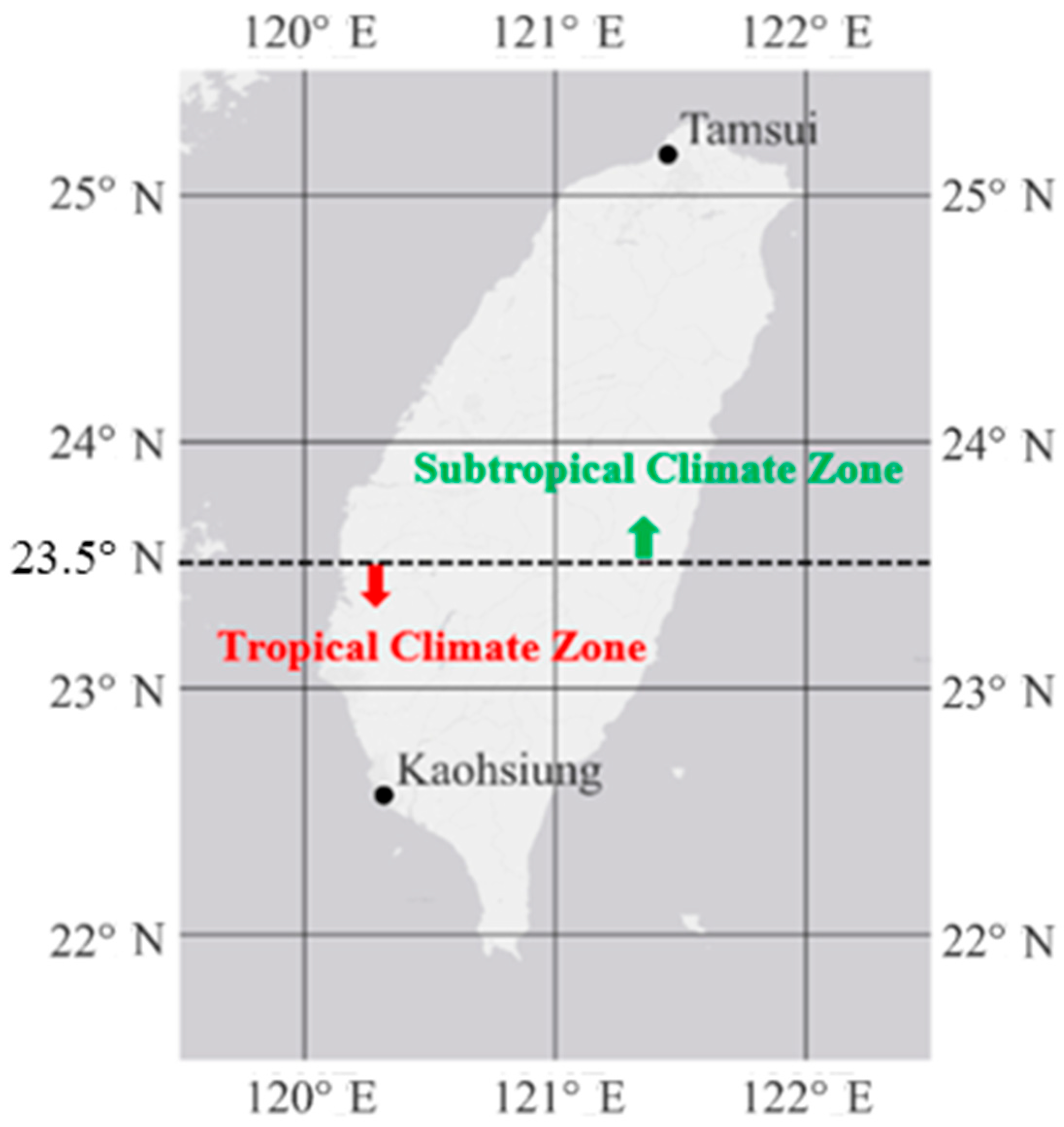
The Tamsui and Kaohsiung in Taiwan are selected as cases to demonstrate the proposed approach. The historical rainfall data were obtained from manual weather stations operated by the Central Weather Administration of Taiwan. Additionally, data from Tamsui Station (hereinafter referred to as “T”) and Kaohsiung Station (hereinafter referred to as “K”) were used as examples for case studies. The locations of these weather stations are shown in Figure 3, and their basic data are provided in Table 2. The dataset spans from January 1950 to December 2005, comprising 672 records by month. Both Tamsui (T) and Kaohsiung (K) are coastal cities located on Taiwan’s western seaboard. Tamsui, situated in the northern part of the island, experiences a subtropical climate zone, while Kaohsiung, in the south, falls within the tropical climate zone. The differences in their climatic and rainfall characteristics are significant, and both stations maintain comprehensive precipitation records. Historical data indicate that Tamsui’s mean annual rainfall is approximately 1500 mm, while Kaohsiung’s is about 2000 mm. Figure 4a presents the monthly mean hyetograph for Tamsui, which does not clearly distinguish between the wet season (October through April of the next year) and the dry season (May through September). In contrast, Figure 4b illustrates the monthly mean hyetograph for Kaohsiung, where the wet and dry seasons are distinctly defined. This disparity arises because the northeast monsoon brings abundant rainfall in winter to windward Tamsui, while Kaohsiung—lying in the monsoon’s rain shadow—receives relatively little winter precipitation. Nevertheless, both stations experience substantial rainfall from summer afternoon thunderstorms and typhoon events. The data were divided into training (TR) and testing (TS) datasets at a 3:1 ratio, as detailed in Table 3.

4. Model Development

4.1. Development Process of the ELADM Model

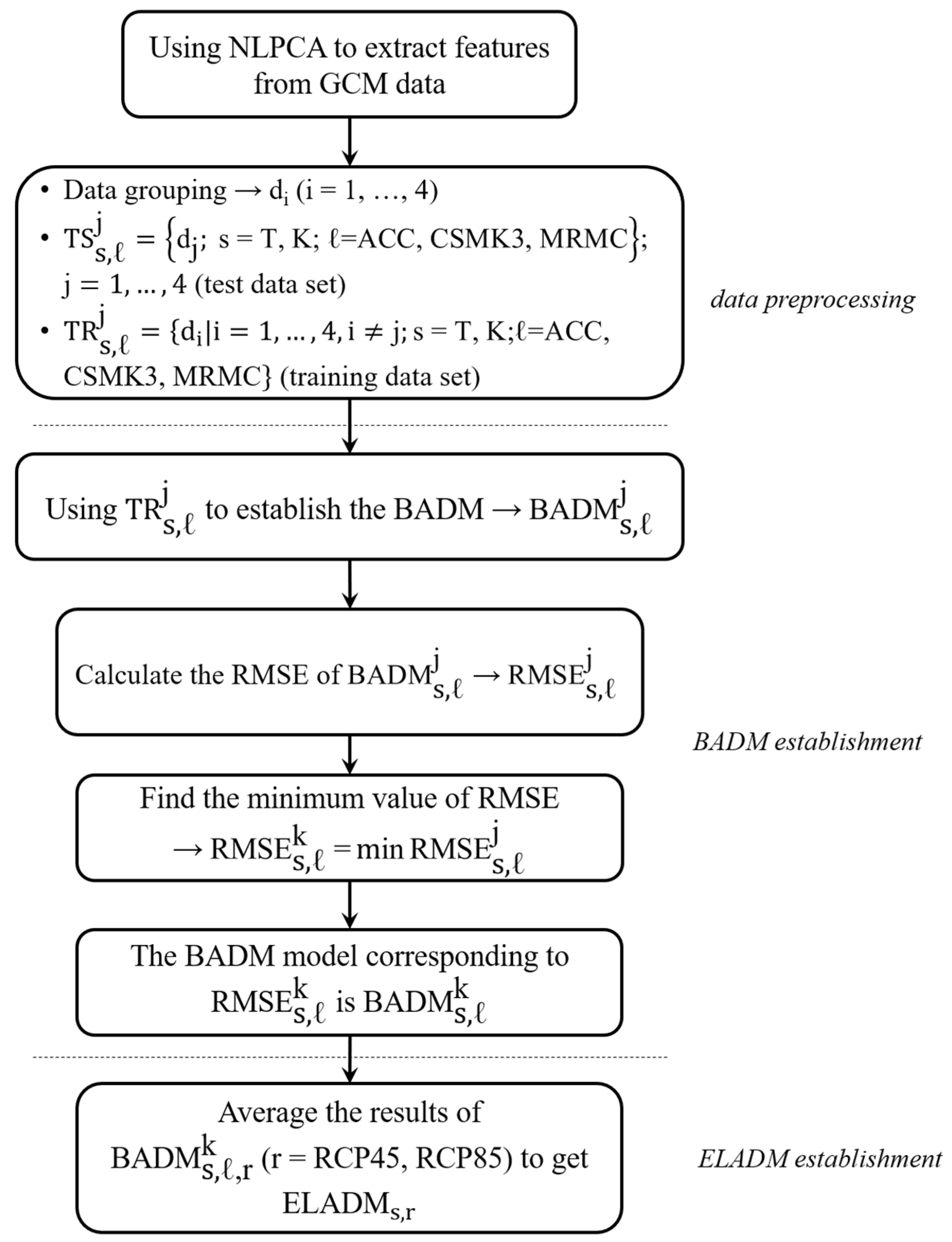
The development process of the ELADM model is illustrated in Figure 5 and consists of the following steps: (1) Applying NLPCA to extract features from GCM data. (2) Dividing the three types of GCM data into four equal parts d i   ( i = 1 ,   ,   4 ) based on the data groups in Table 3. One group j is randomly selected from the same GCM model as test set TS s , l j , while the remaining groups are assigned as training set TR s , l j to establish BADM s , l i , where the subscript s represents different stations (s = T, K) and l the different GCM models ( l = ACC, CSMK3, MRMC). Three GCM models are used to establish the BADM model ( BADM s , l j ), where j represents the TR data from the GCM model used in developing the BADM model. (3) Calculating the RMSE ( RMSE s , l j ) of the testing data TS s , l j in the BADM s , l j model, where the BADM model with the lowest RMSE is designated as BADM s , l k . (4) Averaging the simulation results ( 1 3 BADM s , l , r k ) from the two future emission scenarios (RCP 4.5 and RCP 8.5) of the optimal BADM model ( BADM s , l k ) to obtain the final ELADM model ( ELADM s , r for s = T, K).
The core of the BADM l i model is ANFIS, which was implemented in this study using the ANFIS function in MATLAB version 2016b. The parameters requiring optimization include the number of training iterations and the MFs count. The parameter optimization process for the BADM model is as follows: First, the gbellmf (bell function) is used as the MFs in this study. Second, the number of training iterations is determined, with each model trained using iterations of 15, 30, 50, 100, 150, 200, 250, and 300 as comparative variables. Next, the number of MFs is set between 2 and 4. Finally, the predicted values are compared with actual observations to compute the RMSE, with the model achieving the lowest RMSE selected as the optimal BADM model.
For the ELADM model considering future emission scenarios, using Tamsui (T) and RCP 4.5 (RCP 45) as an example, the prediction results of the optimal BADM models for ACC, CSMK3, and MRMC form the ELADM model for the Tamsui Station under the RCP 4.5 emission scenario, represented as ELADM T ,   RCP 45 .

4.2. Selection of the Number of Nonlinear Principal Components

The number of input variables in this study ranges from 12 to 23, depending on the GCM model used. The complexity and noise in the original GCM data may impact the prediction performance of the BADM model. Therefore, NLPCA is applied in this study for variable feature extraction. Before performing the NLPCA analysis, the original data must undergo normalization (z-score). This process enhances the model’s iteration speed, reduces gradient descent time, and retains and scales the inter-factor features, thereby improving model accuracy. Table 4 presents the results of the nonlinear principal component analysis for the ACC model ( BADM T , A C C 4 ) at the Tamsui Station. The number of input variables was reduced from 19 to 4 by retaining components that collectively accounted for 90% of the cumulative explained variance. The penalty values, hidden layer neurons, HIC, variance ratio, and cumulative explained variance ratio corresponding to the nonlinear principal component 4 are 0.01, 4, 0.288, 4.08, and 90.161%, respectively. For the CSMK3 and MRMC models at Tamsui, the selected input variable factors are 3 and 6, respectively. At Kaohsiung, the selected input variable factors for the ACC, CSMK3, and MRMC models are 5, 4, and 6, respectively.

4.3. Performance Evaluation of the BADM Model

In this study, the ELADM model was developed by averaging the prediction results of the BADM model and the optimal BADM model. The evaluation results of the BADM model are presented in Table 5. For the Tamsui Station, the datasets used in the ACC, CSMK3, and MRMC models correspond to the fourth group (TR: 1964/01–2005/12; TS: 1950/01–1963/12). The optimal setting for the number of MFs for the Bell function is 2, with the RMSE (111.58 mm) of BADM T , A C C 4 showing the best performance. In contrast, the BADM K , C S M K 3 3 model for Kaohsiung demonstrates the best performance, with an RMSE of 122.93 mm. As shown in Table 5, the model with the fewest NLPCs achieves the best prediction performance, while the model with the most NLPCs exhibits the poorest prediction performance.

4.4. Evaluation of Historical Scenario Performance of the Optimal BADM Model

This study employed the optimal BADM model among three GCM models to simulate historical rainfall predictions. The prediction results were then compared with actual historical rainfall trends to evaluate the model’s performance, as illustrated in Figure 6. The figure presents a comparison of rainfall for Tamsui (Figure 6a) and Kaohsiung (Figure 6b). Regardless of the model used, the simulation results closely align with historical rainfall trends, with Kaohsiung predictions outperforming those of Tamsui. This difference may be attributed to the greater rainfall variance between the wet and dry seasons in Kaohsiung, which allows the ANFIS model to learn the spatiotemporal distribution of precipitation more distinctly. In contrast, Tamsui experiences less pronounced seasonal rainfall variation, potentially leading to larger simulation errors for the MRMC model compared to the other two models. In summary, Figure 6 shows that the downscaling results of the three GCM models (ACCESS, CSMK3, MRMC) closely follow historical data trends at the Kaohsiung Station, whereas greater variance is observed at the Tamsui Station, particularly with significant prediction deviations in rainfall during July and August for the MRMC model. The results indicate that the performance of downscaling models at different stations may be influenced by local precipitation characteristics.

5. Results and Discussions

5.1. Monthly Precipitation Evaluation for Future Scenarios

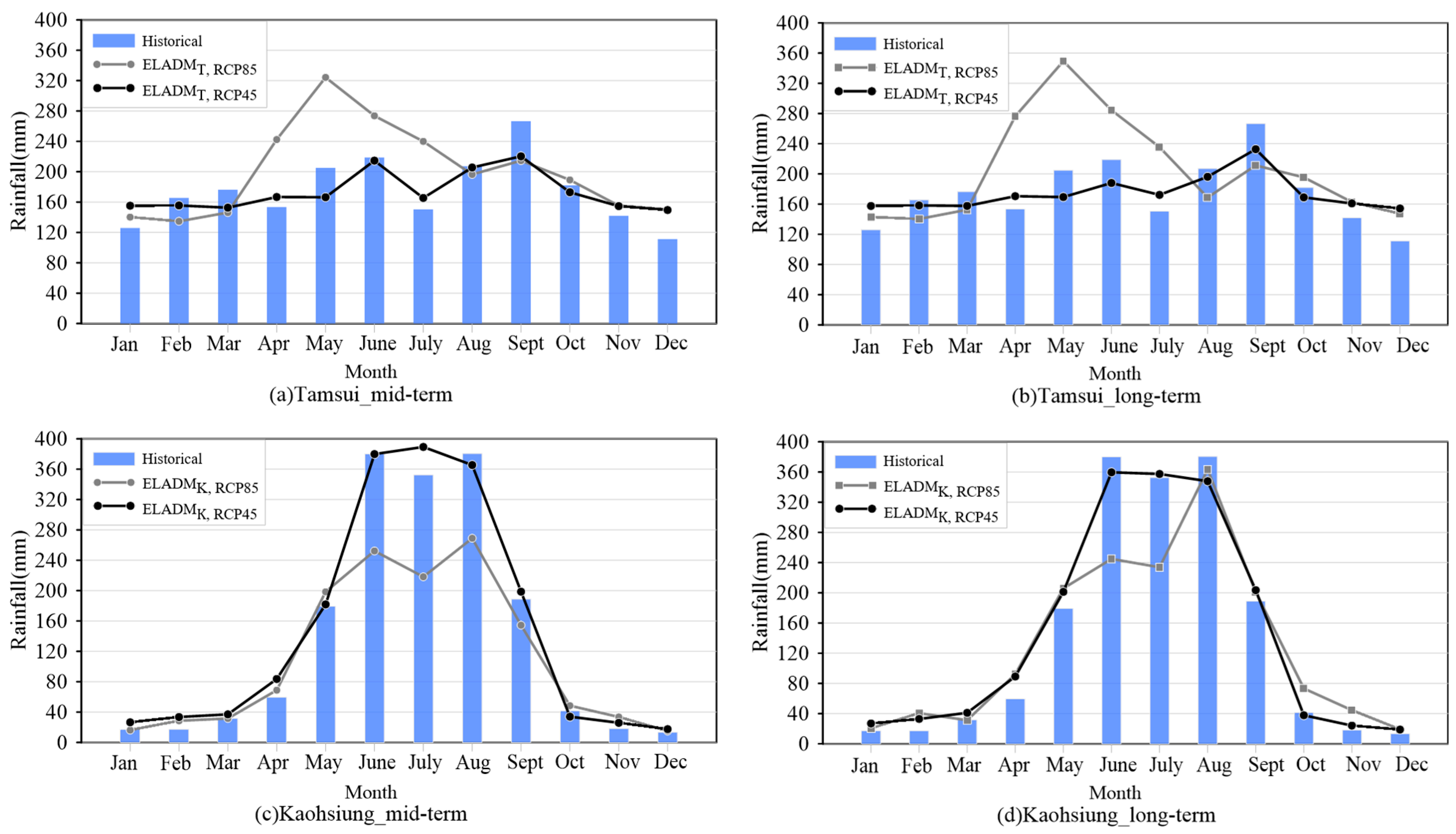
In this study, the optimal model from each category was used to simulate rainfall under various future emission scenarios (RCP45 and RCP 85). The averaged results were compared with historical rainfall trends, as shown in Figure 7. Overall, the future scenario models under RCP45 closely resemble historical rainfall patterns. Comparing the trend of future scenarios under the RCP 85 emission scenario with historical rainfall, a significant difference is observed between the simulation results and historical conditions in the mid-term and long-term for Tamsui (April to July) and Kaohsiung (June to August), largely attributed to the inferior simulation performance of the MRMC model. The significant variability of simulated precipitation observed in MRMC may stem from the MRMC model’s physical parameterizations, which struggle to accurately capture the effects of Taiwan’s complex, small-scale topography under the winter northeast monsoon. This suggests that future changes in northeast monsoon characteristics—driven by climate change—could substantially alter rainfall patterns in subtropical regions.

5.2. Exceeding Probiblity of Precipitation for Future Scenarios

This study analyzed the exceedance probabilities of monthly rainfall simulated under the ELADM model for future scenarios of RCP45 and RCP85 scenarios against historical average rainfall, as shown in Figure 8. Tamsui exhibits similar mid-term and long-term rainfall trends, with exceedance probabilities fluctuating significantly between 0% and 100%, likely due to subtle changes in monthly rainfall. The greatest discrepancy in exceedance probabilities for mid-term RCP45 and RCP85 occurs between May and June, though the overall differences remain relatively indistinct. The long-term trend in Tamsui is similar to the mid-term trend, but differences between RCP45 and RCP85 are more pronounced. Conversely, Kaohsiung shows significant differences between mid-term and long-term trends, with exceedance probabilities ranging between 40% and 80%, likely due to the pronounced rainfall differences between wet and dry seasons. During wet seasons, exceedance probabilities in Kaohsiung are lower, while they are higher during dry seasons. The mid-term discrepancies between RCP45 and RCP85 in Kaohsiung are considerable, while the long-term trends for RCP45 and RCP85 exhibit less distinction. In summary, future scenarios indicate a high risk of exceedance probabilities during the dry seasons of Kaohsiung. Under future warming, subtropical regions such as Tamsui may experience shifts in northeast monsoon seasonality, potentially delaying its onset and intensifying its strength, which could lead to greater variability in monthly rainfall anomalies. In tropical areas like Kaohsiung, warming may increase the likelihood of enhanced winter precipitation more so than in summer. Variations in the frequency or duration of typhoons over Taiwan could influence summer rainfall patterns, suggesting that tropical regions may undergo significant changes in both winter and summer precipitation regimes, with serious implications for water resource management.

5.3. Evaluation of Uncertainitu of Precipitation Under Future Scenarios

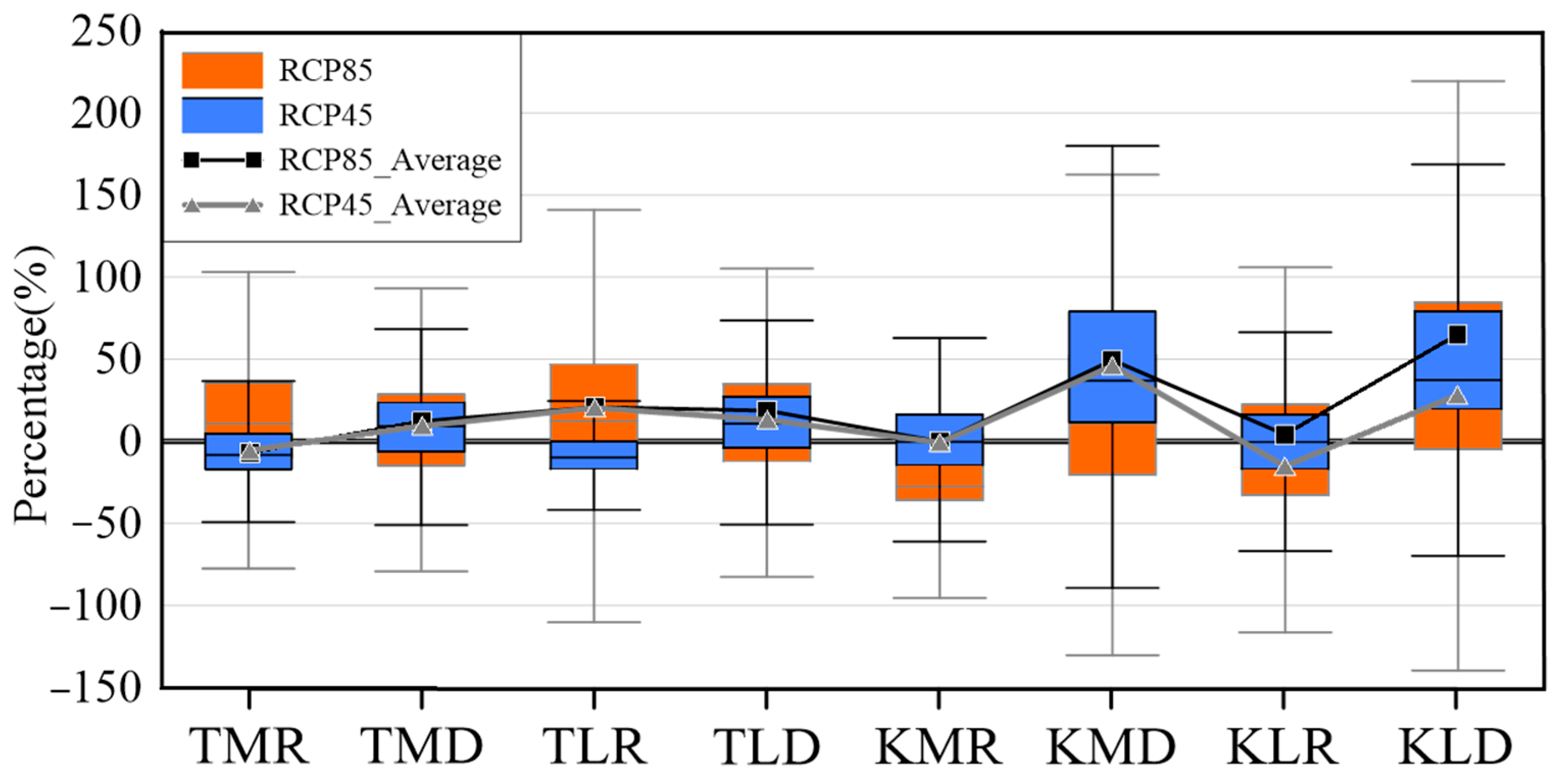
In this study, the percentage increase or decrease in monthly rainfall under future RCP45 and RCP85 scenarios, simulated using the ELADM model, was calculated relative to historical average rainfall to evaluate future rainfall variability in wet and dry seasons. Box plots illustrate these data, with T and K representing the Tamsui Station and the Kaohsiung Station, M and L indicating mid-term and long-term periods, and R and D denoting wet and dry seasons, respectively, as shown in Figure 9. In the figure, TMR represents Tamsui’s mid-term wet seasons, while KLD represents Kaohsiung’s long-term dry seasons, and so forth.
Overall, Tamsui exhibits smaller percentage fluctuations than Kaohsiung, indicating a lower probability of extreme precipitation events in the future. However, Tamsui shows considerable rainfall variability in long-term wet seasons, while Kaohsiung experiences minor percentage changes in wet seasons but greater variances in dry seasons, with a wider fluctuation range for upper and lower limits. This suggests a higher probability of extreme rainfall events during dry seasons, accompanied by greater rainfall variances. In summary, Tamsui’s relatively small percentage fluctuations may result from less pronounced rainfall differences between wet and dry seasons, while Kaohsiung’s larger variances in rainfall during both seasons may be due to significant predicted percentage fluctuations caused by minimal rainfall during dry seasons. Regarding model uncertainties, the ELADM mitigates uncertainties inherent in both the model and observational data via an ensemble learning approach proposed in the study. However, because different scenarios and GCMs employ distinct assumptions and physical parameters, the results remain strongly dependent on the chosen GCMs and scenario inputs. Overall, the variability of extreme rainfall in the subtropical region (Tamsui) is smaller than in the tropical region (Kaohsiung).

6. Conclusions

This study integrated NLPCA, ANFIS, and EL to develop the ELADM model with ensemble features. NLPCA is employed to extract nonlinear features from complex datasets, thereby reducing the complexity of the ANFIS model and mitigating its sensitivity to data noise. Subsequently, an EL algorithm is applied to enhance the model’s reliability. This approach addresses the limitations commonly encountered in traditional downscaling methods, particularly when applied to regions with complex climatic characteristics. The results of this study can serve as a valuable reference for risk assessment in water resource management. The ELADM model was then used to investigate future rainfall trends and uncertainties for Tamsui and Kaohsiung in Taiwan. Based on the case study and analysis, the following conclusions can be drawn:
  • With the use of NLPCA for nonlinear data feature extraction, the number of original features in the three GCM models was reduced from between 12 and 23 to between 3 and 6 NLPCs through nonlinear dimensionality reduction, achieving a cumulative explained variance ratio of 93.5%. This demonstrates that NLPCA effectively reduces nonlinear dimensionality in the data.
  • The GCM data used for constructing the BADM models for Tamsui and Taichung reveal that the MRMC exhibits significantly larger errors, a higher number of NLPCA components, and greater variability and uncertainty.
  • Under the future RCP 4.5 scenario, rainfall trends are similar to historical rainfall characteristics, with relatively low uncertainty. However, under the RCP 8.5 scenario, significant differences are observed between future mid- and long-term rainfall trends and historical patterns during the wet season in both Tamsui and Kaohsiung. This indicates that the RCP 8.5 scenario could lead to greater variability in wet-season rainfall across northern and southern Taiwan, highlighting the need for proactive planning in water resource management.
  • In both Tamsui and Kaohsiung, the future exceedance probabilities of monthly rainfall show higher probability in the dry season and lower probability in the wet season, regardless of the future time horizon (mid- or long-term) or scenario (RCP 4.5 or RCP 8.5). This suggests an elevated risk of increased rainfall during the dry season and a heightened risk of reduced rainfall during the wet season in the future.
  • With the ELADM model, GCM mid-term and long-term rainfall variances were predicted, and the percentage increase or decrease relative to historical rainfall was calculated. The results indicate that regardless of emission scenarios (RCP 4.5 and RCP 8.5), the ELADM model shows higher rainfall variability in dry seasons compared to wet seasons in Kaohsiung, highlighting the need to improve prevention against potential climate change-induced disaster risks during dry seasons.
  • The BADM models developed using the EL algorithm exhibit smaller RMSE, indicating higher model reliability. This approach can also be applied to future rainfall projections in other regions.

7. Limitations and Future Work

This study utilizes GCM models from CMIP 5, as suggested by the Water Resources Agency of the Ministry of Economic Affairs, Taiwan (WRA), for future water resource assessments, while accounting for the climatic variations influenced by the Central Mountain Range at the same latitude. Further investigation is required in other areas. Future research will use CMIP 6 data to explore the impacts and compare the differences.

Author Contributions

Conceptualization, S.-S.L. and K.-Y.Z.; formal analysis S.-S.L. and K.-Y.Z.; funding acquisition, S.-S.L.; methodology, S.-S.L., C.-P.Y., M.-Y.L. and K.-Y.Z.; resources, S.-S.L. and K.-Y.Z.; supervision, S.-S.L.; writing—original draft, S.-S.L. and K.-Y.Z.; writing—review and editing, S.-S.L., K.-Y.Z. and C.-Y.W.; format analysis, C.-Y.W. All authors have read and agreed to the published version of the manuscript.

Funding

This research and the APC were funded by the Taiwan National Science and Technology Council grant number 113-2625-M033-001.

Institutional Review Board Statement

Not applicable.

Informed Consent Statement

Not applicable.

Data Availability Statement

GCM data are available on the Data Distribution Centre’s website (https://www.ipcc-data.org/sim/gcm_monthly/AR5/, accessed on 30 March 2025). The rainfall data of the stations in Tamsui and Kaohsiung are available on the Taiwan’s Central Weather Administration’s website (https://www.cwa.gov.tw/V8/C/, accessed on 28 May 2025).

Acknowledgments

The support from Project No. 113-2625-M033-001- under the National Science and Technology Council, Taiwan for research projects is greatly appreciated for the completion of this study.

Conflicts of Interest

The authors declare no conflicts of interest. The funders had no role in the design of the study; in the collection, analyses, or interpretation of data; in the writing of the manuscript; or in the decision to publish the results.

References

  1. Lin, L.Y.; Lin, C.T.; Chen, Y.M.; Cheng, C.T.; Li, H.C.; Chen, W.B. The Taiwan climate change projection information and adaptation knowledge platform: A decade of climate research. Water 2022, 14, 358. [Google Scholar] [CrossRef]
  2. Khadka, D.; Babel, M.S.; Abatan, A.A.; Collins, M. An evaluation of CMIP5 and CMIP6 climate models in simulating summer rainfall in the Southeast Asian monsoon domain. Int. J. Climatol. 2022, 42, 1181–1202. [Google Scholar] [CrossRef]
  3. Zhang, K.M.; Fan, G.Z. CMIP5 model for surface temperature simulation and estimation in Qinghai-Tibet plateau region. Plateau Mt. Meteorol. Res. 2021, 41, 80–89. Available online: http://www.gysdqxyj.cn/article/doi/10.3969/j.issn.1674-2184.2021.01.011 (accessed on 26 May 2025).
  4. Lin, S.S.; Hu, Y.L.; Zhu, K.Y. Downscaling model for rainfall based on the influence of typhoon under climate change. J. Water Clim. Change 2022, 13, 2443–2458. [Google Scholar] [CrossRef]
  5. Lin, S.S.; Yeh, W.L.; Zhu, K.Y.; Ho, Y.D.; Wu, W.C. Applying the Deep Neural Network to Estimate Future Trend and Uncertainty of Rainfall under Climate Change. Res. Sq. 2022. [Google Scholar] [CrossRef]
  6. Lin, S.S.; Zhu, K.Y.; Wang, C.Y. A Deep Learning-Based Downscaling Method Considering the Impact on Typhoons to Future Precipitation in Taiwan. Atmosphere 2024, 15, 371. [Google Scholar] [CrossRef]
  7. Lin, S.S.; Zhu, K.Y.; Huang, H.Y. Integration of deep learning neural networks and feature-extracted approach for estimating future regional precipitation. Atmosphere 2025, 16, 165. [Google Scholar] [CrossRef]
  8. Wu, H.J.; Ye, X.D.; Zhang, B.Y.; Chen, B. Assessment of uncertainty propagation from climate modeling to hydrologic forecasting under changing climatic conditions. J. Environ. Inform. 2025, 45, 27. [Google Scholar] [CrossRef]
  9. Zhou, Y.; Guo, S.; Chang, F.J. Explore an evolutionary recurrent ANFIS for modelling multi-step-ahead flood forecasts. J. Hydrol. 2019, 570, 343–355. [Google Scholar] [CrossRef]
  10. Zhou, Y.; Chang, F.J.; Guo, S.; Ba, H.; He, S. A robust recurrent anfis for modeling multi-step-ahead flood forecast of three gorges reservoir in the yangtze river. Hydrol. Earth Syst. Sci. Discuss. 2017, 2017, 1–29. [Google Scholar] [CrossRef]
  11. Bakare, M.S.; Abdulkarim, A.; Shuaibu, A.N.; Muhamad, M.M. Enhancing solar power efficiency with hybrid GEP ANFIS MPPT under dynamic weather conditions. Sci. Rep. 2025, 15, 5890. [Google Scholar] [CrossRef] [PubMed]
  12. Achouri, M.; Zennir, Y.; Tolba, C. Adaptive hybrid ANFIS-PSO and ANFIS-GA approach for occupational risk prediction. Int. J. Occup. Saf. Ergon. 2025, 1–15. [Google Scholar] [CrossRef]
  13. Li, C.; Li, Z.; Jun, X.; Pi, W. The impact of data quality on neural network models. In Cyber Security Intelligence and Analytics; Springer International Publishing: Berlin/Heidelberg, Germany, 2020; pp. 657–665. [Google Scholar] [CrossRef]
  14. Gharawi, A.A.; Alsubhi, J.; Ramaswamy, L. Impact of labeling noise on machine learning: A cost-aware empirical study. In Proceedings of the 2022 21st IEEE International Conference on Machine Learning and Applications (ICMLA), Nassau, Bahamas, 12–14 December 2022; pp. 936–939. [Google Scholar] [CrossRef]
  15. Soni, A.; Arora, C.; Kaushik, R.; Upadhyay, V. Evaluating the impact of data quality on machine learning model performance. J. Nonlinear Anal. Optim. 2023, 14, 0013–0018. [Google Scholar] [CrossRef]
  16. Jang, J.S. ANFIS: Adaptive-network-based fuzzy inference system. IEEE Trans. Syst. Man Cybern. 1993, 23, 665–685. [Google Scholar] [CrossRef]
  17. Hsieh, W.W. Nonlinear principal component analysis of noisy data. Neural Netw. 2007, 20, 434–443. [Google Scholar] [CrossRef] [PubMed]
  18. Schapire, R.E. The strength of weak learnability. Mach. Learn. 1990, 5, 197–227. [Google Scholar] [CrossRef]
  19. Wolpert, D.H. Stacked generalization. Neural Netw. 1992, 5, 241–259. [Google Scholar] [CrossRef]
  20. Breiman, L. Bagging predictors. Mach. Learn. 1996, 24, 123–140. [Google Scholar] [CrossRef]
  21. Das, J.; Manikanta, V.; Nikhil Teja, K.; Umamahesh, N.V. Two decades of ensemble flood forecasting: A state-of-the-art on past developments, present applications and future opportunities. Hydrol. Sci. J. 2022, 67, 477–493. [Google Scholar] [CrossRef]
  22. Manikanta, V.; Teja, K.N.; Das, J.; Umamahesh, N.V. On the verification of ensemble precipitation forecasts over the Godavari River basin. J. Hydrol. 2023, 616, 128794. [Google Scholar] [CrossRef]
  23. Kramer, M.A. Nonlinear principal component analysis using autoassociative neural networks. AIChE J. 1991, 37, 233–243. [Google Scholar] [CrossRef]
  24. Hsieh, W.W. Nonlinear multivariate and time series analysis by neural network methods. Rev. Geophys. 2004, 42. [Google Scholar] [CrossRef]
  25. Hsieh, W.W. Nonlinear principal component analysis: A new information criterion for model selection in noisy climate datasets (Invited Speaker). In Proceedings of the Fifth Conference on Artificial Intelligence Applications to Environmental Science, Antonio, TX, USA, 14–18 January 2007; Available online: https://ams.confex.com/ams/87ANNUAL/webprogram/Paper116761.html (accessed on 26 May 2025).
  26. Sugeno, M. An introductory survey of fuzzy control. Inf. Sci. 1985, 36, 59–83. [Google Scholar] [CrossRef]
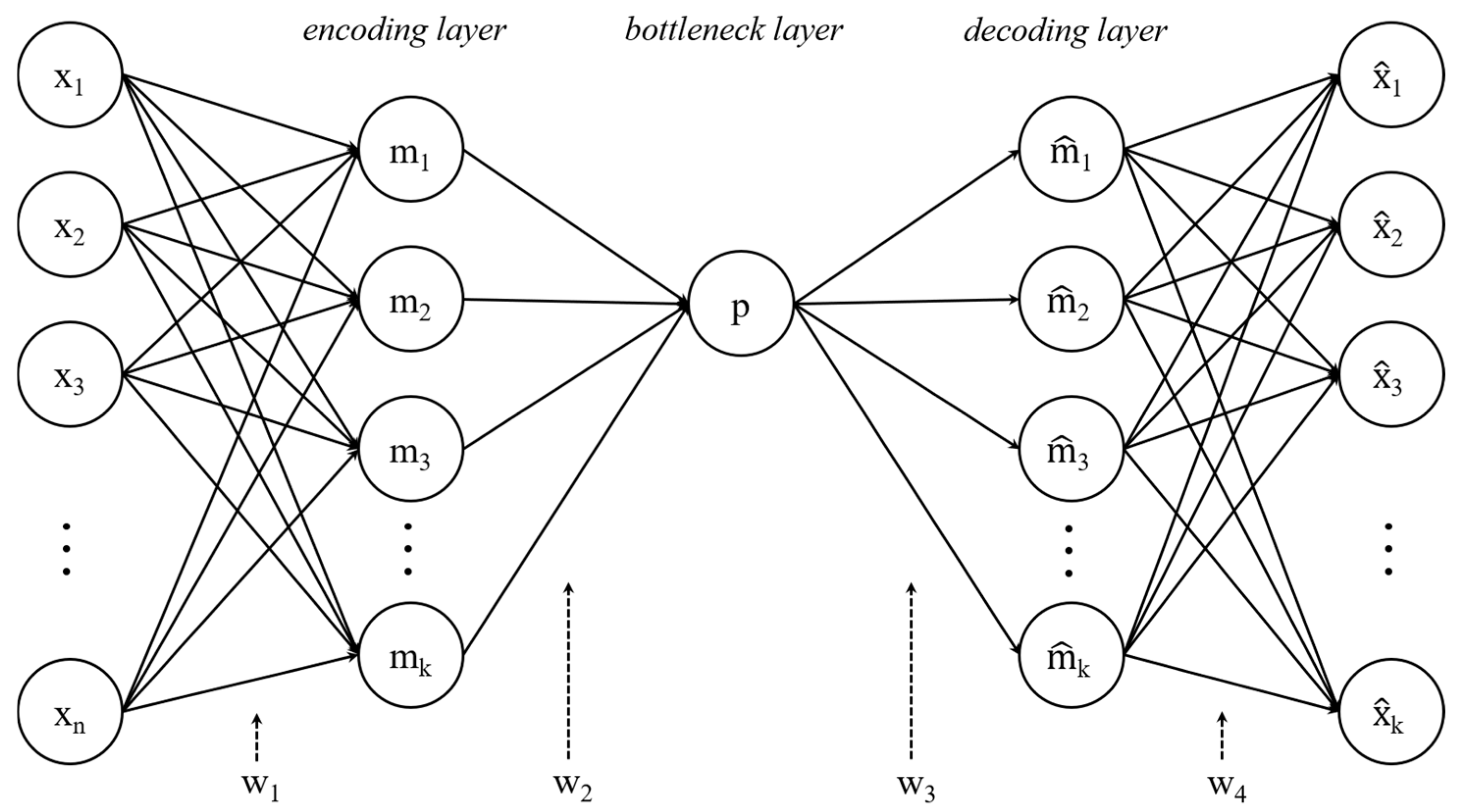
Figure 1. NN architecture of NLPCA.
Atmosphere 16 00669 g001
Figure 2. ANFIS architecture.
Atmosphere 16 00669 g002
Figure 3. Locations and climate zones of Tamsui and Kaohsiung.
Atmosphere 16 00669 g003
Figure 4. Historical monthly hyetographs for Tamsui (a) and Kaohsiung (b) Stations.
Atmosphere 16 00669 g004
Figure 5. ELADM model development flowchart.
Atmosphere 16 00669 g005
Figure 6. Evaluating BADM under historical scenarios against historical monthly averages at (a) Tamsui and (b) Kaohsiung (1964–1977).
Atmosphere 16 00669 g006
Figure 7. Evaluating BADM under future emission scenarios against historical monthly averages in Tamsui (a,b) and Kaohsiung (c,d): Mid-Term (2061–2080) vs. Long-Term (2081–2100).
Atmosphere 16 00669 g007
Figure 8. Exceedance probabilities of the ELADM models (P represents the exceedance probability): (a,c) Mid-Term (2061–2080) vs. (b,d) Long-Term (2081–2100).
Atmosphere 16 00669 g008
Figure 9. Comparing ELADM (boxplots) and best BADM (line plot with markers) outputs for future emission scenario rainfall in wet and dry seasons.
Atmosphere 16 00669 g009
Table 1. Basic information of selected GCM data.
ModelsAbbreviationResolutionNumber of VariablesHistorical Data LengthData Length of
Mid-Term Scenario
Data Length of
Long-Term Scenario
ACCESS1.0ACC192 (km) × 145 (km)191950/01–2005/122061/01–2080/122081/01–2100/12
CSIRO-MK3.6.0CSMK3192 (km) × 96 (km)121950/01–2005/122061/01–2080/122081/01–2100/12
MRI-CGCM3MRMC320 (km) × 160 (km)231950/01–2005/122061/01–2080/122081/01–2100/12
Table 2. Basic data of stations.
Station NameStation CodeCoordinateData PeriodDuration (Month)
Tamsui 466900 (121°26′24″ E, 25°09′56″ N) 1950/01–2005/12 672
Kaohsiung 467440 (120°18′29″ E, 22°34′04″ N) 1950/01–2005/12 672
Table 3. Training and Testing Datasets.
Station NameGCMGroup NumberDuration of TRDuration of TS
TamsuiACC11950/01–1991/121992/01–2005/12
21950/01–1977/12, 1992/01–2005/121978/01–1991/12
31950/01–1963/12, 1978/01–2005/121964/01–1977/12
41964/01–2005/121950/01–1963/12
CSMK311950/01–1991/121992/01–2005/12
21950/01–1977/12, 1992/01–2005/121978/01–1991/12
31950/01–1963/12, 1978/01–2005/121964/01–1977/12
41964/01–2005/121950/01–1963/12
MRMC11950/01–1991/121992/01–2005/12
21950/01–1977/12, 1992/01–2005/121978/01–1991/12
31950/01–1963/12, 1978/01–2005/121964/01–1977/12
41964/01–2005/121950/01–1963/12
KaohsiungACC11950/01–1991/121992/01–2005/12
21950/01–1977/12, 1992/01–2005/121978/01–1991/12
31950/01–1963/12, 1978/01–2005/121964/01–1977/12
41964/01–2005/121950/01–1963/12
CSMK311950/01–1991/121992/01–2005/12
21950/01–1977/12, 1992/01–2005/121978/01–1991/12
31950/01–1963/12, 1978/01–2005/121964/01–1977/12
41964/01–2005/121950/01–1963/12
MRMC11950/01–1991/121992/01–2005/12
21950/01–1977/12, 1992/01–2005/121978/01–1991/12
31950/01–1963/12, 1978/01–2005/121964/01–1977/12
41964/01–2005/121950/01–1963/12
Table 4. Explanatory data of selected NLPCA meteorological factors (with BADM T , A C C 4 as an example).
Value NumberPenaltymHICTotal Variance (%)Cumulative (%)
NLPC 10.0120.06457.81857.818
NLPC 20.120.13618.05775.875
NLPC 30.140.15910.20686.081
NLPC 40.0140.2884.08090.161
NLPC 5020.5411.78691.947
NLPC 6030.4321.52393.470
Selected NLPC: NLPC 1–NLPC 4.
Table 5. Evaluation of BADM models.
Best BADMMFNLPCRMSE (mm)
BADM T , A C C 4 24111.58
BADM T , C S M K 3 4 23112.64
BADM T , M R M C 4 26127.18
BADM K , A C C 3 25129.08
BADM K , C S M K 3 3 24122.93
BADM K , M R M C 3 26135.58
Disclaimer/Publisher’s Note: The statements, opinions and data contained in all publications are solely those of the individual author(s) and contributor(s) and not of MDPI and/or the editor(s). MDPI and/or the editor(s) disclaim responsibility for any injury to people or property resulting from any ideas, methods, instructions or products referred to in the content.