
Testing the Performance of Large-Scale Atmospheric Indices in Estimating Precipitation in the Danube Basin


Abstract
1. Introduction
2. Data and Methods
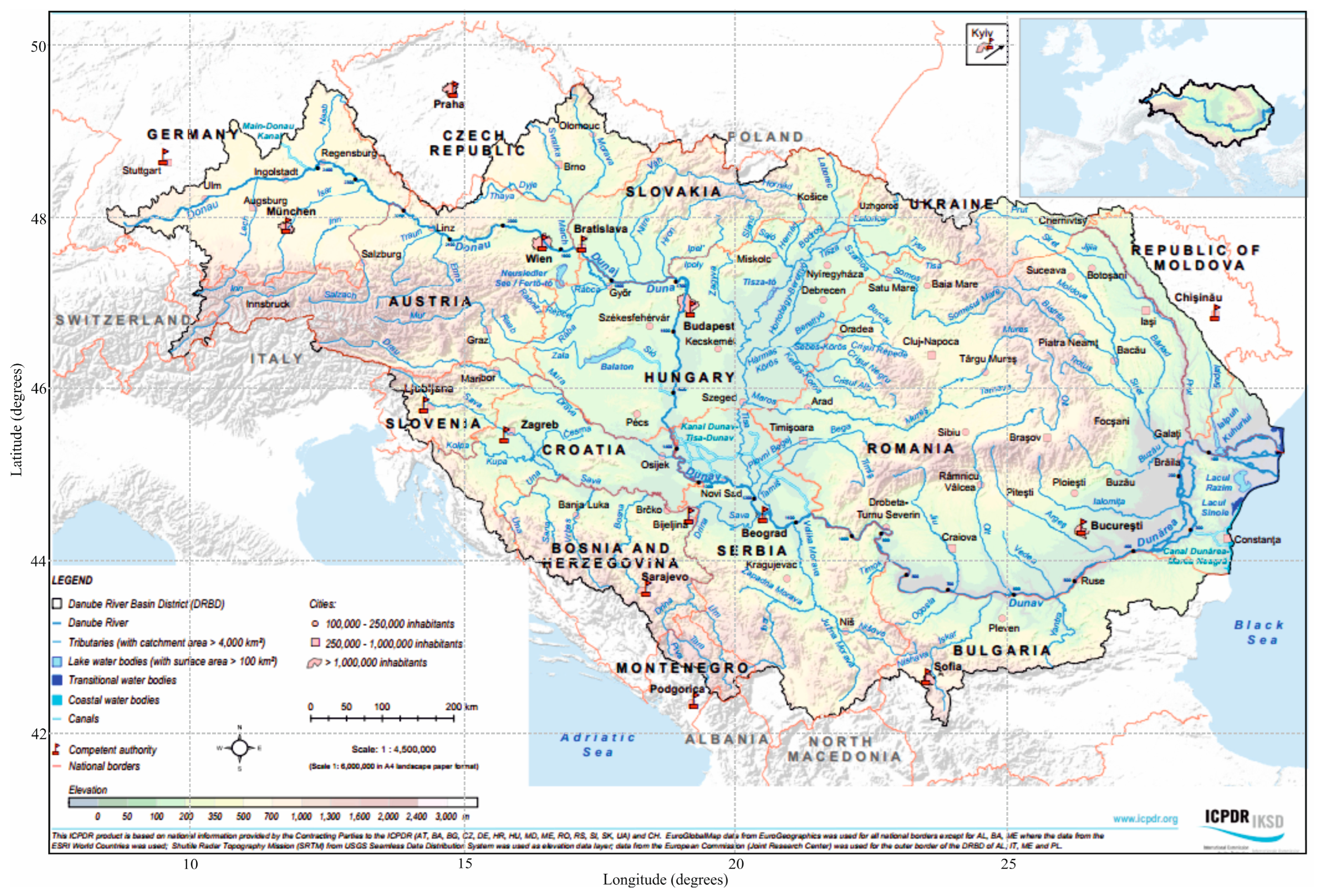
2.1. Data
- -
- The NAOI, obtained from the Hurrell-Station-Based Monthly NAO Index [28].
- -
- The GBOI, introduced by [17]; supplied monthly values for the period 1901–2020 are presented in the Supplementary Materials.
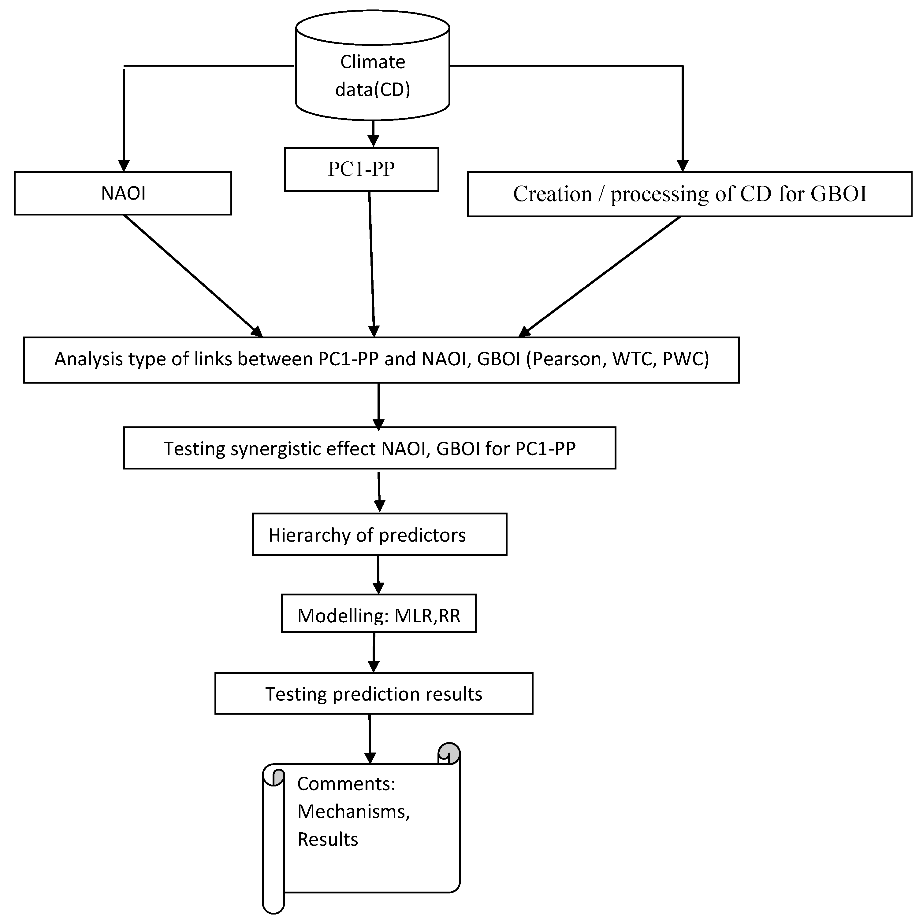
2.2. Methods
3. Results and Discussion
3.1. Bivariate Analyses
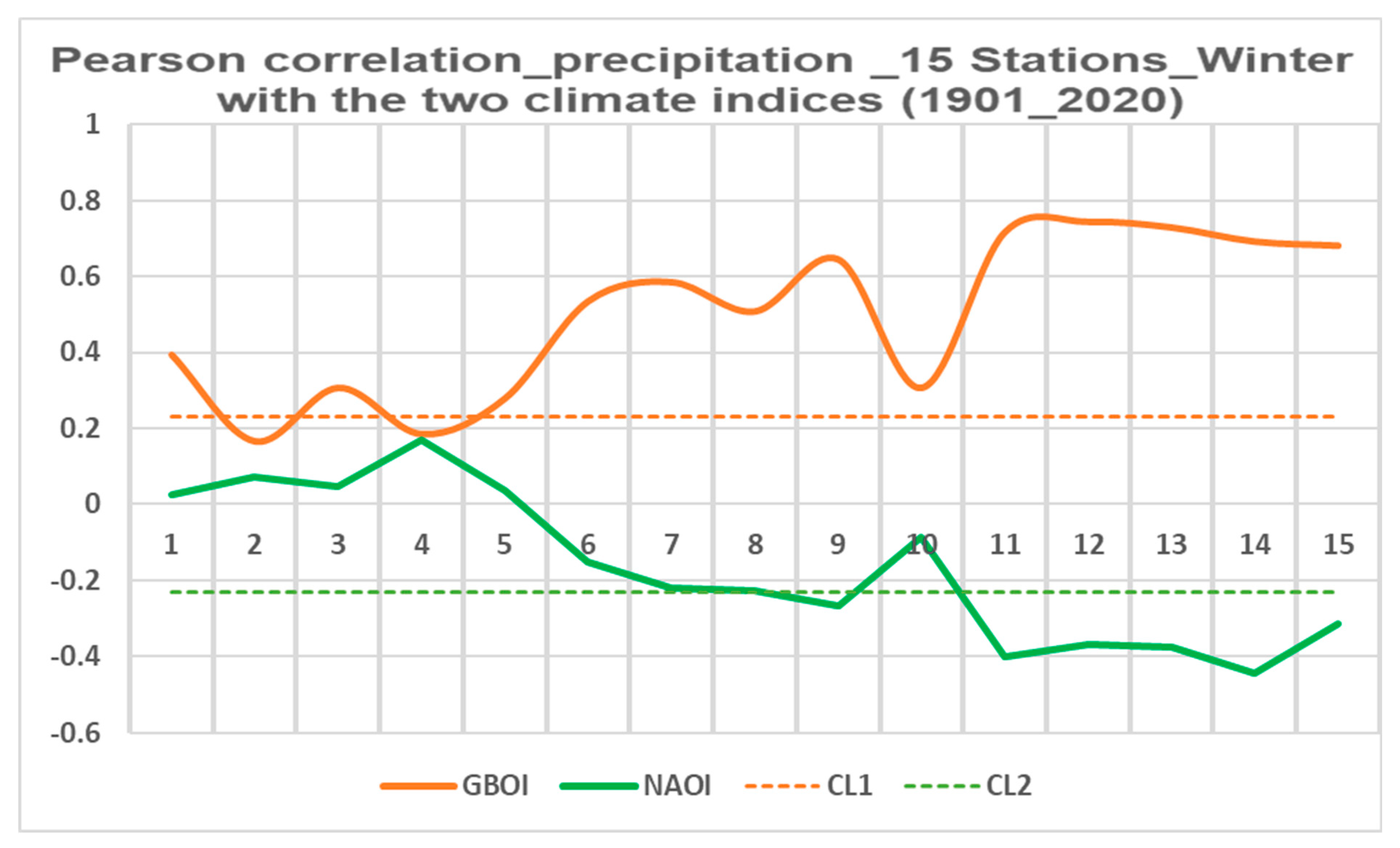
3.1.1. Testing the Links Through Pearson Correlation Coefficients
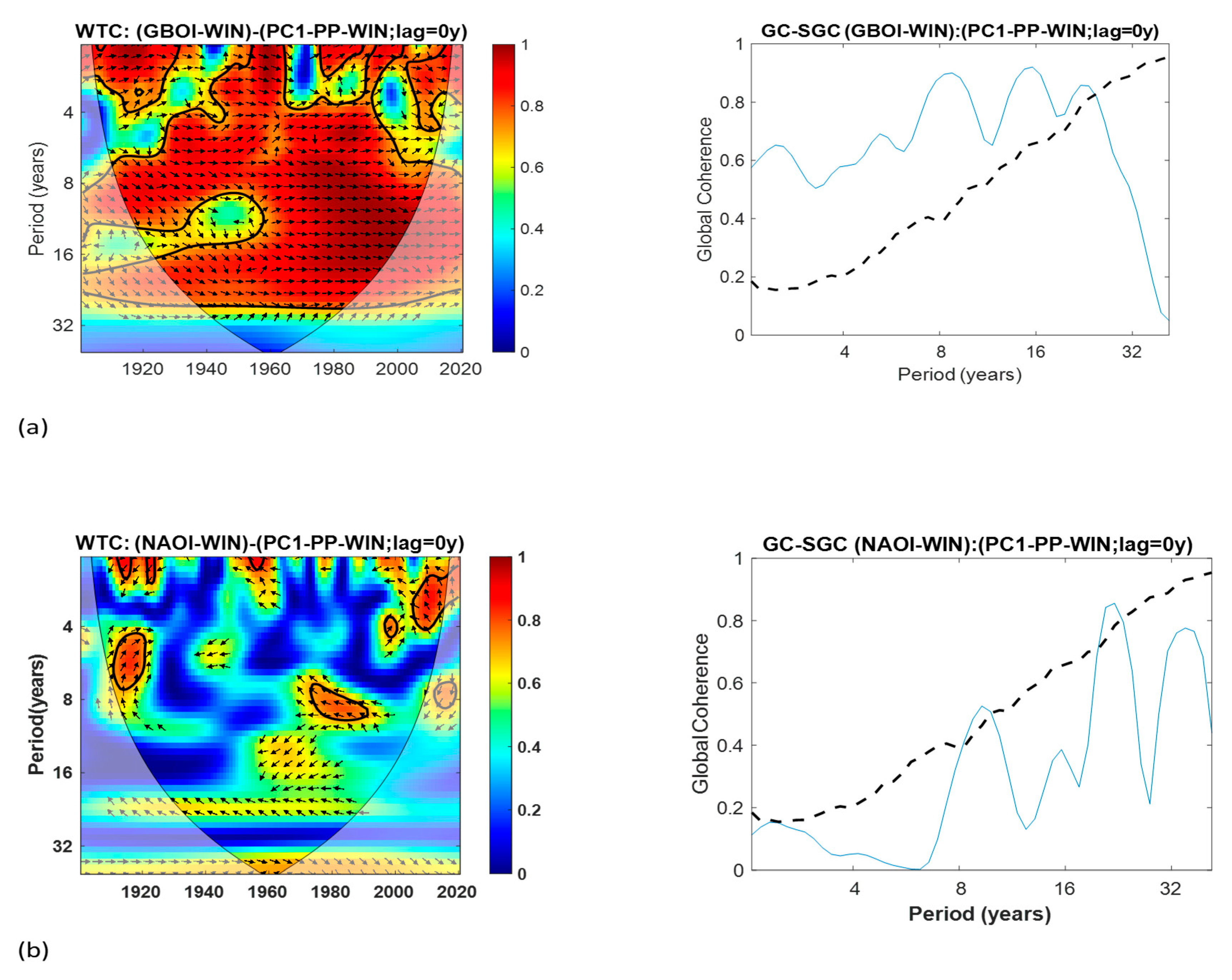
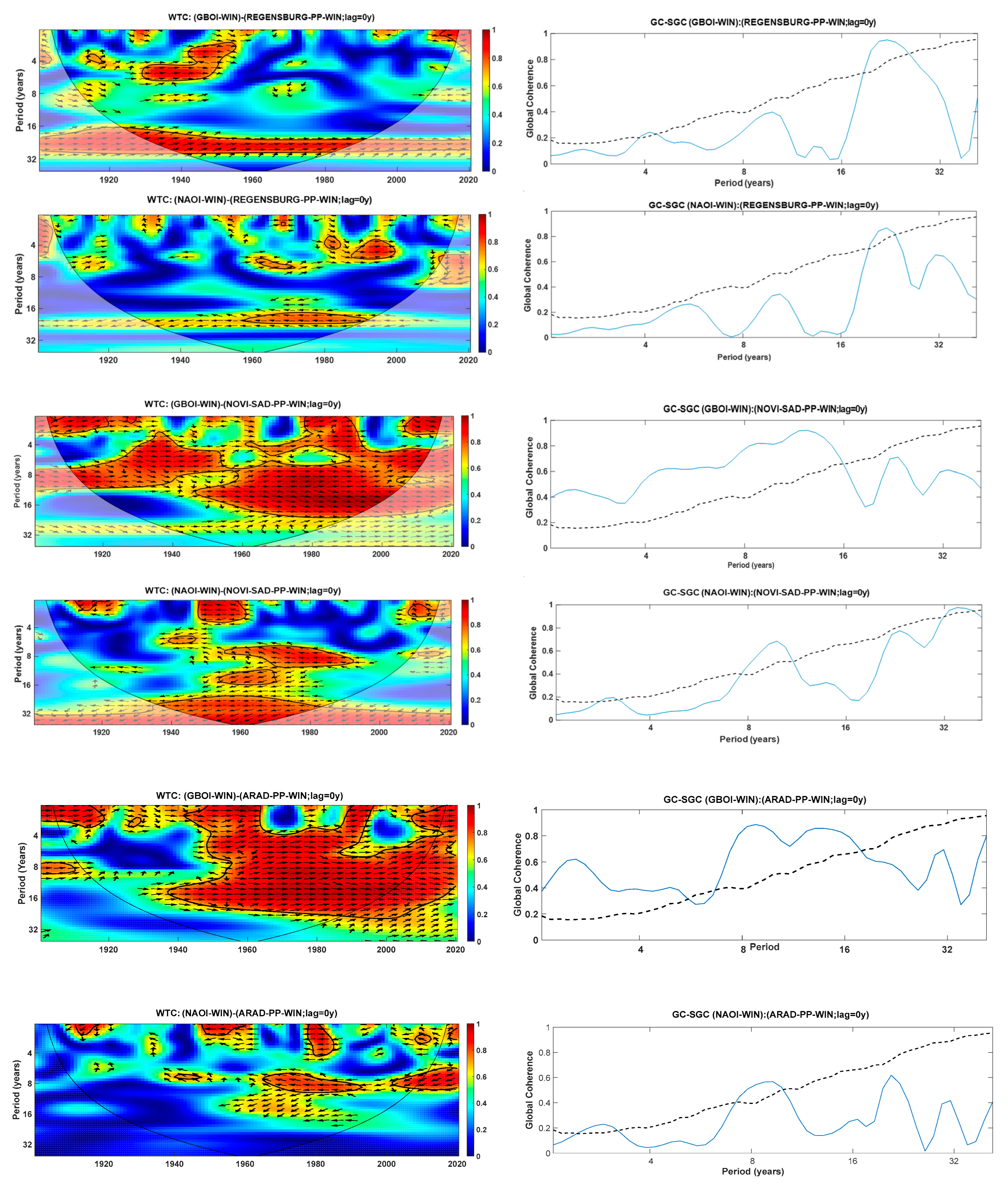
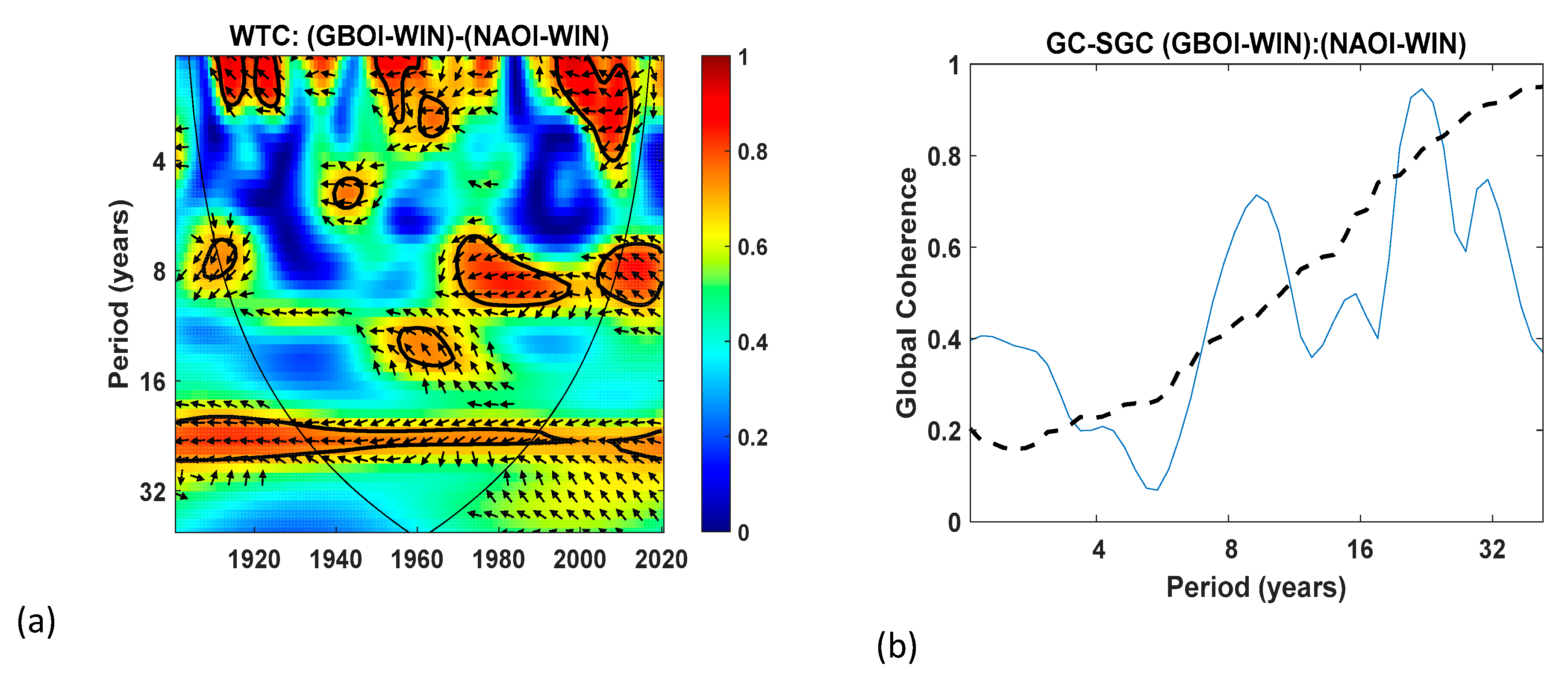
3.1.2. Time–Frequency Domain Analysis
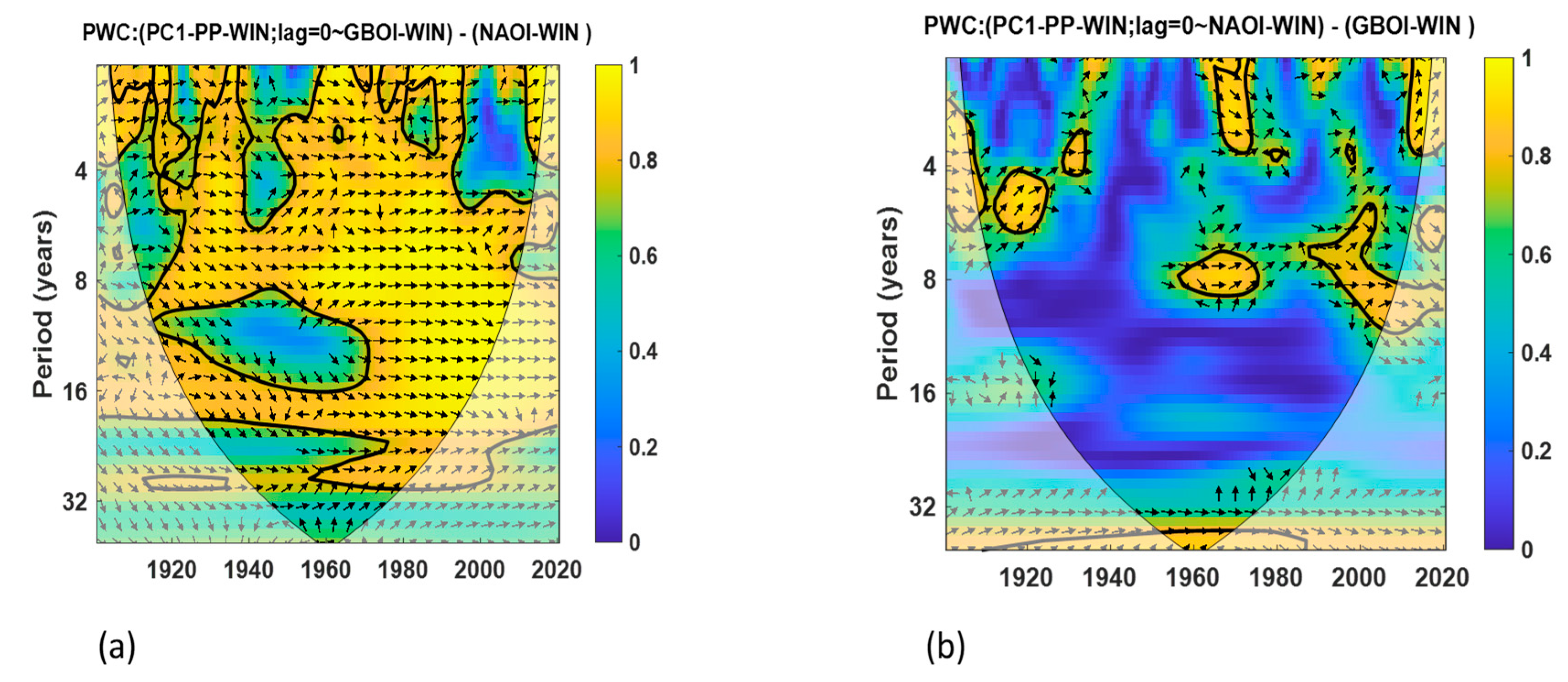
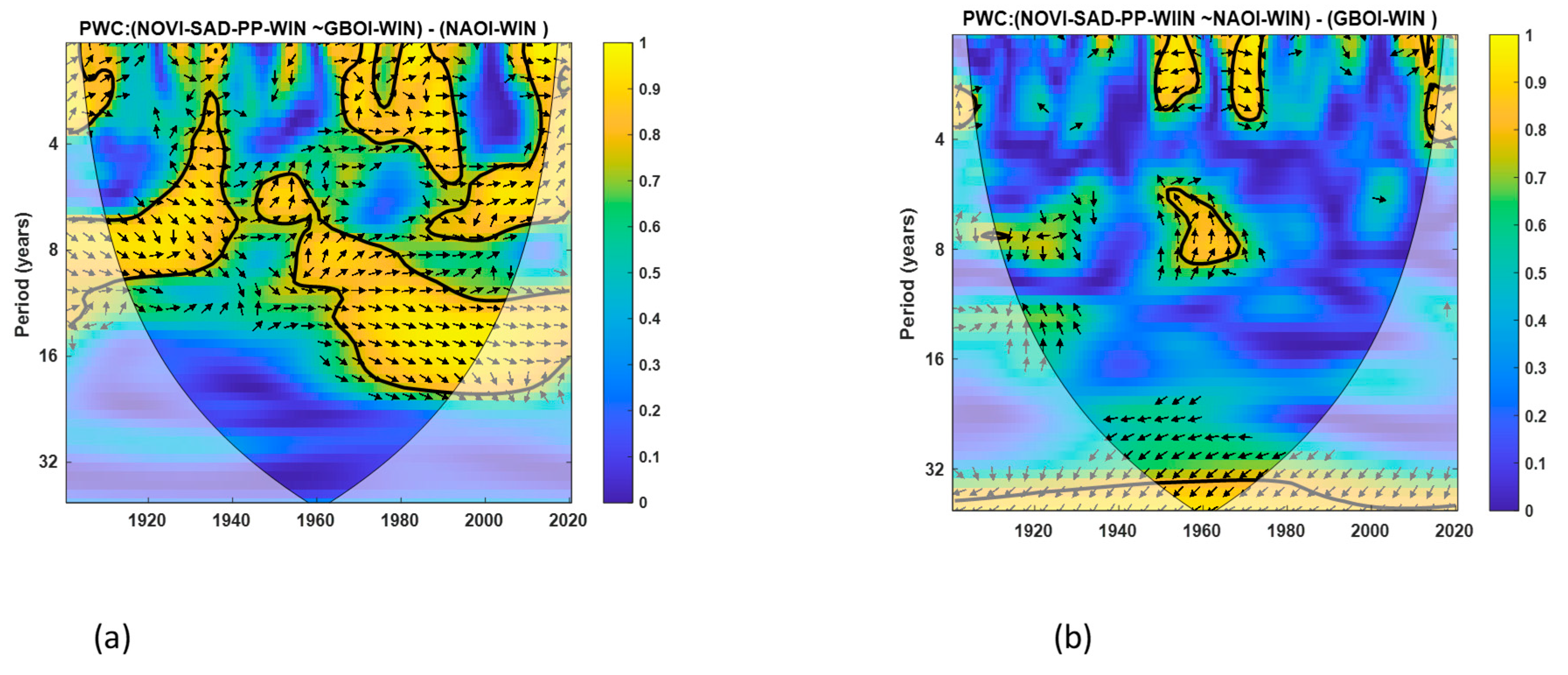
3.2. Partial Wavelet Coherence (PWC) Analyses
3.3. Testing the Combined Influence of GBOI and NAOI on Precipitation in the Danube Basin Through Multiple Linear Regression (MLR)
3.4. Experiments to Eliminate Collinearity Between Predictors
4. Conclusions
Supplementary Materials
Author Contributions
Funding
Institutional Review Board Statement
Informed Consent Statement
Data Availability Statement
Conflicts of Interest
References
- Castellarin, A.; Persiano, S.; Pugliese, A.; Aloe, A.; Skøien, J.O.; Pistocchi, A. Prediction of streamflow regimes over large geographical areas: Interpolated flow–duration curves for the Danube region. Hydrol. Sci. J. 2018, 63, 845–861. [Google Scholar] [CrossRef]
- Tsonis, A.A.; Elsner, J.B. Chaos, strange attractors, and weather. Bull. Am. Meteor. Soc. 1989, 70, 14–23. [Google Scholar] [CrossRef]
- Nicolis, C. Long-term climatic variability and chaotic dynamics. Tellus A Dyn. Met. and Ocean. 1987, 39, 1–9. [Google Scholar] [CrossRef]
- Tang, X.; Li, J. Synergistic effect of boreal autumn SST over the tropical and South Pacific and winter NAO on winter precipitation in the southern Europe. npj Clim. Atmos. Sci. 2024, 7, 78. [Google Scholar] [CrossRef]
- Beniston, M.; Jungo, P. Shifts in the distributions of pressure, temperature and moisture and changes in the typical weather patterns in the Alpine region in response to the behavior of the North Atlantic Oscillation. Theor. Appl. Clim. 2002, 71, 29–42. [Google Scholar] [CrossRef]
- Beniston, M.; Stephenson, D.B.; Christensen, O.B.; Ferro, C.A.; Frei, C.; Goyette, S.; Halsnaes, K.; Holt, T.; Jylhä, K.; Koffi, B.; et al. Future extreme events in European climate: An exploration of regional climate model projections. Clim. Change 2007, 81, 71–95. [Google Scholar] [CrossRef]
- McKenna, C.M.; Maycock, A.C. The role of the North Atlantic Oscillation for projections of winter mean precipitation in Europe. Geophys. Res. Lett. 2022, 49, e2022GL099083. [Google Scholar] [CrossRef]
- Diodato, N.; Seim, A.; Ljungqvist, F.C.; Bellocchi, G. A millennium-long perspective on recent groundwater changes in the Iberian Peninsula. Commun. Earth Environ. 2024, 5, 257. [Google Scholar] [CrossRef]
- Mathbout, S.; Lopez-Bustins, J.A.; Royé, D.; Martin-Vide, J.; Benhamrouche, A. Spatiotemporal Variability of Daily Precipitation Concentration and Its Relationship to Teleconnection Patterns over the Mediterranean during 1975–2015. Int. J. Climatol. 2019, 40, 1435–1455. [Google Scholar] [CrossRef]
- Boughdadi, S.; Ait Brahim, Y.; El Alaoui El Fels, A.; Saidi, M.E. Rainfall Variability and Teleconnections with Large-Scale Atmospheric Circulation Patterns in West-Central Morocco. Atmosphere 2023, 14, 1293. [Google Scholar] [CrossRef]
- Christensen, J.H.; Kanikicharla, K.K.; Aldrian, E.; An, S.I.; Albuquerque Cavalcanti, I.F.; de Castro, M.; Dong, W.; Goswami, P.; Hall, A.; Kanyanga, J.K.; et al. Climate phenomena and their relevance for future regional climate change. In Climate Change 2013—The Physical Science Basis; Cambridge University Press: Cambridge, UK, 2013; Volume 9781107057999, pp. 1217–1308. [Google Scholar] [CrossRef]
- Cohen, J.; Zhang, X.; Francis, J.; Jung, T.; Kwok, R.; Overland, J.; Taylor, P.C.; Lee, S.; Coumou, D.; Handorf, D.; et al. Arctic Change and Possible Influence on Mid-Latitude Climate and Weather: A US CLIVAR White Paper; Uhlenbrock, K., Ed.; U.S. CLIVAR Project Office: Washington, DC, USA, 2018. [Google Scholar] [CrossRef]
- Tošić, I.; Hrnjak, I.; Gavrilov, M.B.; Unkašević, M.; Marković, S.B.; Lukić, T. Annual and seasonal variability of precipitation in Vojvodina, Serbia. Theor. Appl. Climatol. 2014, 117, 331–341. [Google Scholar] [CrossRef]
- Luković, J.; Blagojevć, D.; Kilibarda, M.; Bajat, B. Spatial pattern of North Atlantic Oscillation impact on rainfall in Serbia. Spat. Stat. 2015, 14, 39–52. [Google Scholar] [CrossRef]
- Milošević, D.; Savić, S.; Pantelić, M.; Stankov, U.; Žiberna, I.; Dolinaj, D.; Leščešen, I. Variability of seasonal and annual precipitation in Slovenia and its correlation with large-scale atmospheric circulation. Open Geosci. 2016, 8, 593–605. [Google Scholar] [CrossRef]
- Malinović-Milićević, S.; Mihailović, D.T.; Radovanović, M.M.; Drešković, N. Extreme precipitation indices in Vojvodina region (Serbia). J. Geogr. Inst. Jovan C 2018, 68, 1–15. [Google Scholar] [CrossRef]
- Mares, I.; Mares, C.; Mihailescu, M. Stochastic modeling of the connection between sea level pressure and discharge in the Danube lower basin by means of Hidden Markov Model. EGU Gen. Assem. Conf. Abstr. 2013, 15, 7606. [Google Scholar]
- Mares, I.; Mares, C.; Dobrica, V.; Demetrescu, C. Comparative study of statistical methods to identify a predictor for discharge at Orsova in the Lower Danube Basin. Hydrol. Sci. J. 2020, 65, 371–386. [Google Scholar] [CrossRef]
- Mares, C.; Mares, I.; Dobrica, V.; Demetrescu, C. Discriminant Analysis of the Solar Input on the Danube’s Discharge in the Lower Basin. Atmosphere 2023, 14, 1281. [Google Scholar] [CrossRef]
- Stosic, B.; Stosic, T.; Tosic, I.A.; Djurdjevic, V. Multifractal Analysis of Temperature in Europe: Climate Change Effect. Chaos Solitons Fractals 2025, 196, 116386. [Google Scholar] [CrossRef]
- Benestad, R.E.; Parding, K.M.; Dobler, A. Downscaling the probability of heavy rainfall over the Nordic countries. Hydrol. Earth Syst. Sci. 2025, 29, 45–65. [Google Scholar] [CrossRef]
- Jam-Jalloh, S.U.; Liu, J.; Wang, Y.; Li, Z.; Jabati, N.-M.S. Wavelet Analysis and the Information Cost Function Index for Selection of Calibration Events for Flood. Water 2023, 15, 2035. [Google Scholar] [CrossRef]
- Fadhel, S.; Han, D. On the connection between large-scale climate indices and rainfall variability in Iraq. Dyn. Atmos. Ocean. 2025, 110, 101540. [Google Scholar] [CrossRef]
- Mares, I.; Mares, C.; Dobrica, V.; Demetrescu, C. Selection of Optimal Palmer Predictors for Increasing the Predictability of the Danube Discharge: New Findings Based on Information Theory and Partial Wavelet Coherence Analysis. Entropy 2022, 24, 1375. [Google Scholar] [CrossRef]
- Mares, I.; Dobrica, V.; Mares, C.; Demetrescu, C. Assessing the solar variability signature in climate variables by information theory and wavelet coherence. Sci. Rep. 2021, 11, 11337. [Google Scholar] [CrossRef]
- Mares, I.; Dobrica, V.; Demetrescu, C.; Mares, C. The Combined Effect of Atmospheric and Solar Activity Forcings on the Hydroclimate in Southeastern Europe. Atmosphere 2023, 14, 1622. [Google Scholar] [CrossRef]
- Klein Tank, A.M.G.; Wijngaard, J.B.; Können, G.P.; Böhm, R.; Demaree, G.; Gocheva, A.; Mileta, M.; Pashiardis, S.; Hejkrlik, L.; Kern-Hansen, C.; et al. Daily dataset of 20th-century surface air temperature and precipitation series for the European Climate Assessment. Int. J. Climatol. 2002, 22, 1441–1453. [Google Scholar] [CrossRef]
- Hurrell, J.; Phillips, A. National Center for Atmospheric Research Staff (Eds). Last Modified 2023-07-10 “The Climate Data Guide: Hurrell North Atlantic Oscillation (NAO) Index (Station-Based)”. Available online: https://climatedataguide.ucar.edu/climate-data/hurrell-north-atlantic-oscillation-nao-index-station-based (accessed on 5 February 2025).
- Grinsted, A.; Moore, J.C.; Jevrejeva, S. Application of the cross wavelet transform and wavelet coherence to geophysical time series. Nonlinear Proc. Geophys. 2004, 11, 561–566. [Google Scholar] [CrossRef]
- Schulte, J.; Najjar, R.G.; Li, M. The influence of climate modes on streamflow in the Mid-Atlantic region of the United States. J. Hydrol. Reg. Stud. 2016, 5, 80–99. [Google Scholar] [CrossRef]
- Schulte, J. Global Wavelet Coherence, MATLAB Central File Exchange. Available online: https://www.mathworks.com/matlabcentral/fileexchange/54682-global-wavelet-coherence (accessed on 9 February 2025).
- Hu, W.; Si, B.C. Technical Note: Improved partial wavelet coherency for understanding scale- specific and localized bivariate relationships in geosciences. Hydrol. Earth Syst. Sci. 2021, 25, 321–331. [Google Scholar] [CrossRef]
- Nash, J.E.; Sutcliffe, J.V. River flow forecasting through conceptual models part I—A discussion of principles. J. Hydrol. 1970, 10, 282–290. [Google Scholar] [CrossRef]
- Moriasi, D.N.; Arnold, J.G.; Van Liew, M.W.; Bingner, R.L.; Harmel, R.D.; Veith, T.L. Model evaluation guidelines for systematic quantification of accuracy in watershed simulations. Trans. Asabe 2007, 50, 885–900. [Google Scholar] [CrossRef]
- Alfieri, L.; Pappenberger, F.; Wetterhall, F.; Haiden, T.; Richardson, D.; Salamon, P. Evaluation of ensemble streamflow predictions in Europe. J. Hydrol. 2014, 517, 913–922. [Google Scholar] [CrossRef]
- Mares, I.; Mares, C.; Mihailescu, M. NAO impact on the summer moisture variability across Europe. Phys. Chem. Earth Parts A/B/C 2002, 27, 1013–1017. [Google Scholar] [CrossRef]
- Sreedevi, V.; Adarsh, S.; Nourani, V. Multiscale coherence analysis of reference evapotranspiration of north-western Iran using wavelet transform. J. Water Clim. Change 2022, 13, 505–521. [Google Scholar] [CrossRef]
- Mihanović, H.; Orlie, M.; Pasaria, Z. Diurnal thermocline oscillations driven by tidal flow around an island in the Middle Adriatic. J. Mar. Syst. 2009, 78, S157–S168. [Google Scholar] [CrossRef]
- Gu, X.; Sun, H.; Zhang, Y.; Zhang, S.; Lu, C. Partial Wavelet Coherence to Evaluate Scale-dependent Relationships Between Precipitation/Surface Water and Groundwater Levels in a Groundwater System. Water Resour. Manag. 2022, 36, 2509–2522. [Google Scholar] [CrossRef]
- Zhou, Z.; Liu, S.; Ding, Y.; Fu, Q.; Wang, Y.; Cai, H.; Shi, H. Assessing the responses of vegetation to meteorological drought and its influencing factors with partial wavelet coherence analysis. J. Environ. Manag. 2022, 311, 114879. [Google Scholar] [CrossRef]
- Mohan, M.G.; Fathima, S.; Adarsh, S.; Baiju, N.; Nair, G.A.; Meenakshi, S.; Krishnan, M.S. Analyzing the streamflow teleconnections of greater Pampa basin, Kerala, India using wavelet coherence. Phys. Chem. Earth Parts A/B/C 2023, 131, 103446. [Google Scholar] [CrossRef]
- Shrestha, N. Factor analysis as a tool for survey analysis. Am. J. Appl. Math. Stat. 2021, 9, 4–11. [Google Scholar] [CrossRef]
- Hoerl, A.E.; Kennard, R.W. Ridge Regression: Biased Estimation for Nonorthogonal Problems. Technometrics 1970, 12, 55–67. [Google Scholar] [CrossRef]
- Hoerl, A.E.; Kennard, R.W. Ridge Regression: Applications to Nonorthogonal Problems. Technometrics 1970, 12, 69–82. [Google Scholar] [CrossRef]
- Marquardt, D.W.; Snee, R.D. Ridge Regression in Practice. Am. Stat. 1975, 29, 3–20. [Google Scholar] [CrossRef]
- Yin, Y.; Pena, M. An Imputing Technique for Surface Water Extent Timeseries with Streamflow Discharges. Water 2024, 16, 250. [Google Scholar] [CrossRef]
- Varentsov, M.; Krinitskiy, M.; Stepanenko, V. Machine Learning for Simulation of Urban Heat Island Dynamics Based on Large-Scale Meteorological Conditions. Climate 2023, 11, 200. [Google Scholar] [CrossRef]
- Hoffman, L.; Mazloff, M.R.; Gille, S.T.; Giglio, D.; Heimbach, P. Evaluating the Trustworthiness of Explainable Artificial Intelligence (XAI) Methods Applied to Regression Predictions of Arctic Sea Ice Motion. Artif. Intell. Earth Syst. 2025, 4, e240027. [Google Scholar] [CrossRef]
- Faye, D.; de Andrade, F.M.; Suárez-Moreno, R.; Wane, D.; Hegglin, M.I.; Dieng, A.L.; Kaly, F.; Lguensat, R.; Gaye, A.T. Assessment of machine learning-based approaches to improve sub-seasonal to seasonal forecasting of precipitation in Senegal, EGUsphere. Preprint 2025. [Google Scholar] [CrossRef]

| No. St. | Station | CN | LONG | LAT | Height (m) |
|---|---|---|---|---|---|
| 1. | AUGSBURG | GE | 10.56 | 48.26 | 463 |
| 2. | INNSBRUCK | AT | 11.24 | 47.16 | 577 |
| 3. | REGENSBURG | GE | 12.06 | 49.02 | 365 |
| 4. | SONNBLICK | AT | 12.57 | 47.03 | 3106 |
| 5. | SALZBURG | AT | 13.00 | 47.48 | 437 |
| 6 | KREDARICA | SI | 13.51 | 46.22 | 2514 |
| 7. | LJUBLJANA | SI | 14.31 | 46.04 | 299 |
| 8. | GRAZ | AT | 15.27 | 47.05 | 366 |
| 9. | ZAGREB | HR | 15.58 | 45.49 | 156 |
| 10. | WIEN | AT | 16.21 | 48.14 | 198 |
| 11. | SARAJEVO | BA | 18.23 | 43.51 | 577 |
| 12. | OSIJEK | HR | 18.38 | 45.32 | 88 |
| 13. | NOVI-SAD | RS | 19.51 | 45.20 | 84 |
| 14. | BEOGRAD | RS | 20.28 | 44.48 | 132 |
| 15. | ARAD | RO | 21.21 | 46.08 | 117 |
| CIs/Season | WIN | SPR | SUM | AUTUMN |
|---|---|---|---|---|
| GBOI | 0.7868 | 0.4984 | 0.3149 | 0.5859 |
| NAOI | −0.2997 | −0.0680 | 0.0201 | −0.2332 |
Disclaimer/Publisher’s Note: The statements, opinions and data contained in all publications are solely those of the individual author(s) and contributor(s) and not of MDPI and/or the editor(s). MDPI and/or the editor(s) disclaim responsibility for any injury to people or property resulting from any ideas, methods, instructions or products referred to in the content. |
© 2025 by the authors. Licensee MDPI, Basel, Switzerland. This article is an open access article distributed under the terms and conditions of the Creative Commons Attribution (CC BY) license (https://creativecommons.org/licenses/by/4.0/).
Share and Cite
Mares, C.; Dobrica, V.; Mares, I.; Demetrescu, C. Testing the Performance of Large-Scale Atmospheric Indices in Estimating Precipitation in the Danube Basin. Atmosphere 2025, 16, 667. https://doi.org/10.3390/atmos16060667
Mares C, Dobrica V, Mares I, Demetrescu C. Testing the Performance of Large-Scale Atmospheric Indices in Estimating Precipitation in the Danube Basin. Atmosphere. 2025; 16(6):667. https://doi.org/10.3390/atmos16060667
Chicago/Turabian StyleMares, Constantin, Venera Dobrica, Ileana Mares, and Crisan Demetrescu. 2025. "Testing the Performance of Large-Scale Atmospheric Indices in Estimating Precipitation in the Danube Basin" Atmosphere 16, no. 6: 667. https://doi.org/10.3390/atmos16060667
APA StyleMares, C., Dobrica, V., Mares, I., & Demetrescu, C. (2025). Testing the Performance of Large-Scale Atmospheric Indices in Estimating Precipitation in the Danube Basin. Atmosphere, 16(6), 667. https://doi.org/10.3390/atmos16060667