Article

Simulating Near-Surface Winds in Europe with the WRF Model: Assessing Parameterization Sensitivity Under Extreme Wind Conditions

by
Minkyu Lee
1,
Donggun Oh
1,
Jin-Young Kim
1,* and
Chang Ki Kim
1,2
1
Renewable Energy Big Data Laboratory, Korea Institute of Energy Research, Daejeon 34129, Republic of Korea
2
Department of Energy Engineering, University of Science and Technology, Daejeon 34113, Republic of Korea
*
Author to whom correspondence should be addressed.
Atmosphere 2025, 16(6), 665; https://doi.org/10.3390/atmos16060665
Submission received: 21 March 2025 / Revised: 21 May 2025 / Accepted: 28 May 2025 / Published: 31 May 2025
(This article belongs to the Section Meteorology)

Abstract

:
Accurately simulating near-surface wind speeds is indispensable for wind energy development, particularly under extreme weather conditions. This study utilizes the Weather Research and Forecasting (WRF) model with a 6 km resolution to evaluate 80 m wind speed simulations over Europe, using the ECMWF (European Centre for Medium-Range Weather Forecasts) reanalysis version 5 (ERA5) as initial and lateral boundary conditions. Two cases were analyzed: a normal case with relatively weak winds, and an extreme case with intense cyclonic activity over 7 days, focusing on offshore wind farm regions and validated against Forschungsplattformen in Nord- und Ostsee (FINO) observational data. Sensitivity experiments were conducted by modifying key physical parameterizations associated with wind simulation to assess their impact on accuracy. Results reveal that while the model realistically captured temporal wind speed variations, errors were significantly amplified in extreme cases, with overestimation in weak wind regimes and underestimation in strong winds (approximately 1–3 m/s). The Asymmetrical Convective Model 2 (ACM2) planetary boundary layer (PBL) scheme demonstrated superior performance in extreme cases, while there were no significant differences among experiments under normal cases. These findings emphasize the critical role of physical parameterizations and the need for improved modeling approaches under extreme wind conditions. This research contributes to developing reliable wind speed simulations, supporting the operational stability of wind energy systems.

1. Introduction

Wind energy is a key component of the transition to sustainable energy and one of the most prominent renewable energy sources worldwide. In particular, Europe, with its abundant wind resources, has established itself as a global leader in wind power development. To address climate change and achieve carbon neutrality targets, Europe has steadily increased the share of wind energy in its energy consumption [1]. Wind energy accounts for approximately 20% of Europe’s electricity demand in 2023 [2]. Denmark, in particular, sources more than 50% of its electricity from wind energy, making it the European Union (EU) country with the highest proportion of wind energy utilization. The EU has established strategies to expand renewable energy to achieve carbon neutrality by 2050. Wind energy, particularly offshore wind power, is regarded as a key solution for ensuring both power supply stability and energy security [3].
Extreme winds are a critical meteorological factor that can cause significant threats to the structural stability and operational efficiency of wind power systems [4]. Extreme winds can impose excessive loads on wind turbine blades, towers, and power conversion systems, potentially causing equipment damage or failure, which may lead to the shutdown of entire wind farms [5]. Fluctuations in wind speed under extreme weather conditions can exacerbate power output variability, negatively impacting the stability of power grids [6]. For instance, in August 2024, a turbine at the Dogger Bank, an offshore wind farm in the United Kingdom, experienced a blade failure due to strong winds, raising concerns about turbine durability in extreme weather conditions. Despite these risks, studies on extreme winds remain relatively limited, with most existing research focusing on mean wind speeds or general wind resource assessments [7,8,9,10]. Simulating and predicting extreme wind is particularly challenging due to its highly localized and rare occurrence in both spatial and temporal scales. Therefore, research is essential to better understand the characteristics of extreme wind events and to develop realistic simulations for these conditions.
Recent research has increasingly emphasized the importance of understanding extreme winds and their impacts on wind energy systems. For instance, Hannesdóttir et al. [11] analyzed extreme wind fluctuations characterized by ramp-like increases in wind speed, emphasizing their influence on turbulence estimates and potential implications for wind turbine loads. Similarly, Li et al. [12] conducted a sensitivity analysis of the WRF model over the Baltic Sea, examining various model configurations, including domain setup, sea surface temperature, wave coupling, and boundary conditions, to improve offshore wind modeling. Moreover, Vemuri et al. [13] performed a sensitivity analysis of mesoscale simulations to physics parameterizations over the Belgian North Sea using the WRF model, assessing the impact of different planetary boundary layer (PBL), cumulus, and microphysics schemes on simulated wind direction and speed. Their findings underscore the necessity of selecting appropriate physics configurations to enhance the accuracy of wind simulations under extreme weather conditions. Despite these advancements, gaps remain in systematically evaluating the sensitivity of various physical processes within atmospheric models under normal and extreme wind conditions. This study addresses this gap by conducting a numerical model performance across various physics parameterizations, numerical parameters, and datasets that are closely associated with wind speed simulation.
Producing accurate wind speed information is crucial for the wind energy industry [14]. Numerical Weather Prediction (NWP) models are considered essential tools for understanding and forecasting meteorological phenomena, especially when organizing high-resolution datasets. While observational data provide critical information that can capture localized weather conditions, they are often limited by spatial and temporal constraints, making it challenging to obtain continuous and extensive datasets for specific regions or altitudes. Furthermore, although vertical wind measurements from micrometeorological towers, radiosondes, and wind profilers are available at selected locations, their spatial coverage is limited. This makes it difficult to obtain regionally continuous vertical wind profiles. Reanalysis data, on the other hand, offer spatial continuity and long-term records by analyzing past weather conditions, but they also have limitations in resolution and data accuracy [15]. Although reanalysis data effectively reproduce large-scale pressure patterns, they often struggle to realistically represent localized and fine-scale meteorological phenomena, such as wind speeds in complex mountainous terrains or coastal regions [16]. Therefore, to overcome the limitations of observational and reanalysis data and to acquire more accurate information, high-resolution simulations using NWP models are required.
This study aims to systematically evaluate the sensitivity of near-surface wind speed simulations to various physical processes within the WRF model, focusing on both typical atmospheric conditions and extreme conditions that could significantly impact wind energy systems. Sensitivity experiments are conducted using various NWP physical process parameterizations and sea surface temperature (SST) datasets to investigate their effects on wind speed and produce reliable information. These experiments are designed to identify which physical processes most significantly affect wind speed accuracy. This research addresses the limitations of observational and reanalysis datasets by providing high resolution, model-based wind speed simulations that better capture wind variability, particularly under extreme conditions. The findings can support the design and operational optimization of wind power plants by providing insights into model sensitivity and performance.

2. Methods

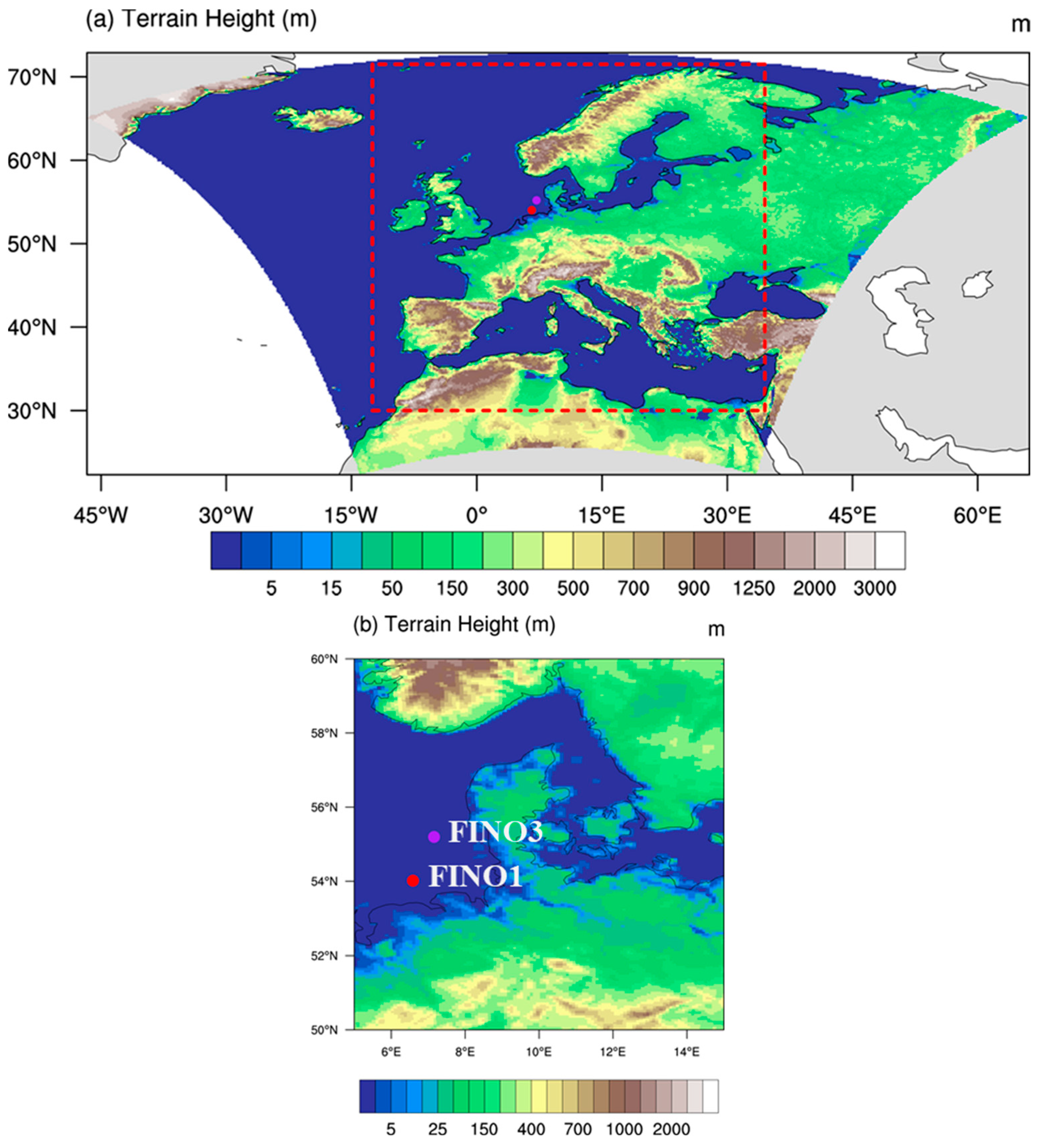
2.1. Data and Model Configuration

Forschungsplattformen in Nord- und Ostsee (FINO) meteorological masts refer to offshore observation platforms located in the German North Sea and Baltic Sea, as shown in Figure 1 [17]. These platforms were established with support from the German Federal Ministry for Economic Affairs and Energy (BMWi) and currently consist of three main stations: FINO1, FINO2, and FINO3. In this study, we used wind speed measurements at a height of 81 m, which closely corresponds to the hub height of typical wind turbines and is therefore most relevant for wind energy applications. The raw wind speed data at FINO platforms are recorded and subsequently averaged to produce 10-min mean values, provided as 10-min averaged values. The FINO datasets undergo quality assurance using a standardized validation tool known as Validaft, which identifies and flags anomalous or unreliable measurements. The datasets are publicly available through the BSH Insitu Portal, managed by the Federal Maritime and Hydrographic Agency (BSH) of Germany (https://www.bsh.de (accessed on 29 March 2025)). FINO masts provide data to support wind resource assessment, the design and optimization of wind power systems, and climate change research.
The Weather Research and Forecasting (WRF) model, one of the widely used meteorological models for simulating atmospheric phenomena, was employed in this study [18]. ERA5 reanalysis data from the European Centre for Medium-Range Weather Forecasts (ECMWF) were used as initial and boundary conditions for WRF model forcing [19]. The ERA5 dataset has a horizontal resolution of 0.25° (~31 km) and provides global atmospheric coverage. The vertical structure consists of 37 pressure levels, ranging from 1000 hPa to 1 hPa. These data were applied as forcing at 3-h intervals throughout the simulation period. The model domain was configured to cover most of Europe, similar to the EURO-Coordinated Regional Climate Downscaling Experiment (CORDEX) domain [20]. The horizontal resolution was set to 6 km, with grid dimensions of 837 and 879 in the east-west and north-south directions, respectively. The reference experiment (REF) prescribed high-resolution global Operational Sea Surface Temperature and Sea Ice Analysis (OSTIA) data with a horizontal resolution of approximately 6 km [21]. The following physical parameterization schemes were utilized for the simulations: Kain–Fritsch convection scheme [22], Yonsei University (YSU) planetary boundary layer scheme [23,24], WSM 6 (WRF single-moment 6-class) microphysics scheme [25], Unified Noah land-surface model [26], revised Mesoscale Model version 5 (MM5) surface layer [27], and Rapid Radiative Transfer Model for General circulation model (RRTMG) shortwave and longwave radiation schemes [28]. The configuration of the REF experiment is described in Table 1. The spectral nudging technique was applied to ensure that the large-scale fields from the reanalysis data influenced not only the boundaries but also the interior of the model domain [29].

2.2. Experimental Design

Wind speeds in Europe are significantly more intense in winter compared to summer [30]. Two cases, representing normal and extreme wind conditions, were selected based on minimum sea level pressure patterns [13,31]. The case was selected from January, the month with the strongest winds in Europe, in 2023. Each simulation period was set to 8 days, with the first day considered as a spin-up period and the other 7 days designated for analysis. Previous studies have suggested that simulation periods longer than one week for wind data production can cause unrealistic results, even though spectral nudging is applied continuously [32]. The simulation period of a normal case is from 21 January 2023 at 00 UTC to 29 January 2023 at 00 UTC. During this period, a strong high-pressure system was present over the Atlantic, North Sea, and Baltic Sea, resulting in a lack of strong winds near the areas where the FINO platforms are located (Figure 2b). The extreme case starts on 7 January 2023 at 00 UTC and ends on 15 January 2023 at 00 UTC. During this period, an intense cyclonic circulation developed over the Atlantic, producing severe winds along the coasts of the United Kingdom, Germany, and Denmark, where many offshore wind farms are concentrated, as well as near the FINO platforms [33]. Furthermore, the United Kingdom faced significant flooding due to heavy precipitation (reported by https://floodlist.com/europe/united-kingdom/flood-risk-somerset-levels-january-2023 (accessed on 29 March 2025)).
This study aims to identify which physics parameterization schemes are more influential in 80 m wind speed simulations and to determine the optimal configuration using various experiments. The schemes, datasets, and levels used in the sensitivity experiments are described in Table 2. First, SST can directly influence the wind simulation in the WRF model through thermal instability, atmospheric mixing, and pressure gradients [34,35]. Thermal gradients forced by SST or convection triggered by heat transfer through air–sea interactions may induce convergence in near-surface winds [36,37]. Additionally, thermal imbalances generated by SST can drive phenomena that can change wind speeds, such as land–sea breezes [38].
The cumulus parameterization scheme (CPS) governs vertical motion and the associated mixing between the lower and middle atmosphere. Strong upward motions can redistribute momentum across different heights, leading to changes in wind patterns near the surface. This effect is particularly pronounced in extreme cases, such as tropical cyclones, extratropical cyclones, and extreme precipitation events, and exhibits sensitivity depending on the specific scheme employed [39,40,41,42,43]. The PBL scheme is one of the most critical factors influencing near-surface wind simulations. The PBL scheme characterizes turbulent mixing processes in the lower atmosphere, calculating momentum, heat, and moisture transport. When turbulence is robust, momentum exchange between layers becomes more active, allowing more intense winds from upper levels to mix downward, potentially increasing wind speeds near the surface [44]. These processes significantly impact the speed, direction, and vertical distribution of near-surface winds [45,46]. The microphysics scheme (MPS), which simulates processes related to clouds, precipitation, and atmospheric moisture changes, primarily covers precipitation and thermodynamic processes. However, these processes can indirectly influence near-surface wind simulations, particularly under extreme wind conditions [47,48]. The land surface model (LSM) simulates interactions between the land surface and the atmosphere, significantly contributing to near-surface wind simulations. The LSM estimates energy exchange, moisture flux, and friction at the surface, processes that can directly influence near-surface wind speed [49]. Furthermore, it incorporates surface characteristics (e.g., vegetation cover, soil type, surface moisture) to derive atmospheric-surface friction, surface roughness, and other factors affecting wind.
The number of vertical levels (VERTs), while not a physical parameterization, plays a crucial role in near-surface wind simulations (about 80 to 150 m), as it can influence local wind patterns, terrain effects, and the thickness of the PBL. High-resolution vertical levels are required for simulating extreme winds [50]. However, more vertical levels do not guarantee better results; the distribution must be appropriately adjusted to the simulation environment and the specific target of the study [51]. Experiments will be conducted to evaluate the sensitivity of the aforementioned schemes and identify the most influential factors focusing on extreme wind simulations.

3. Results

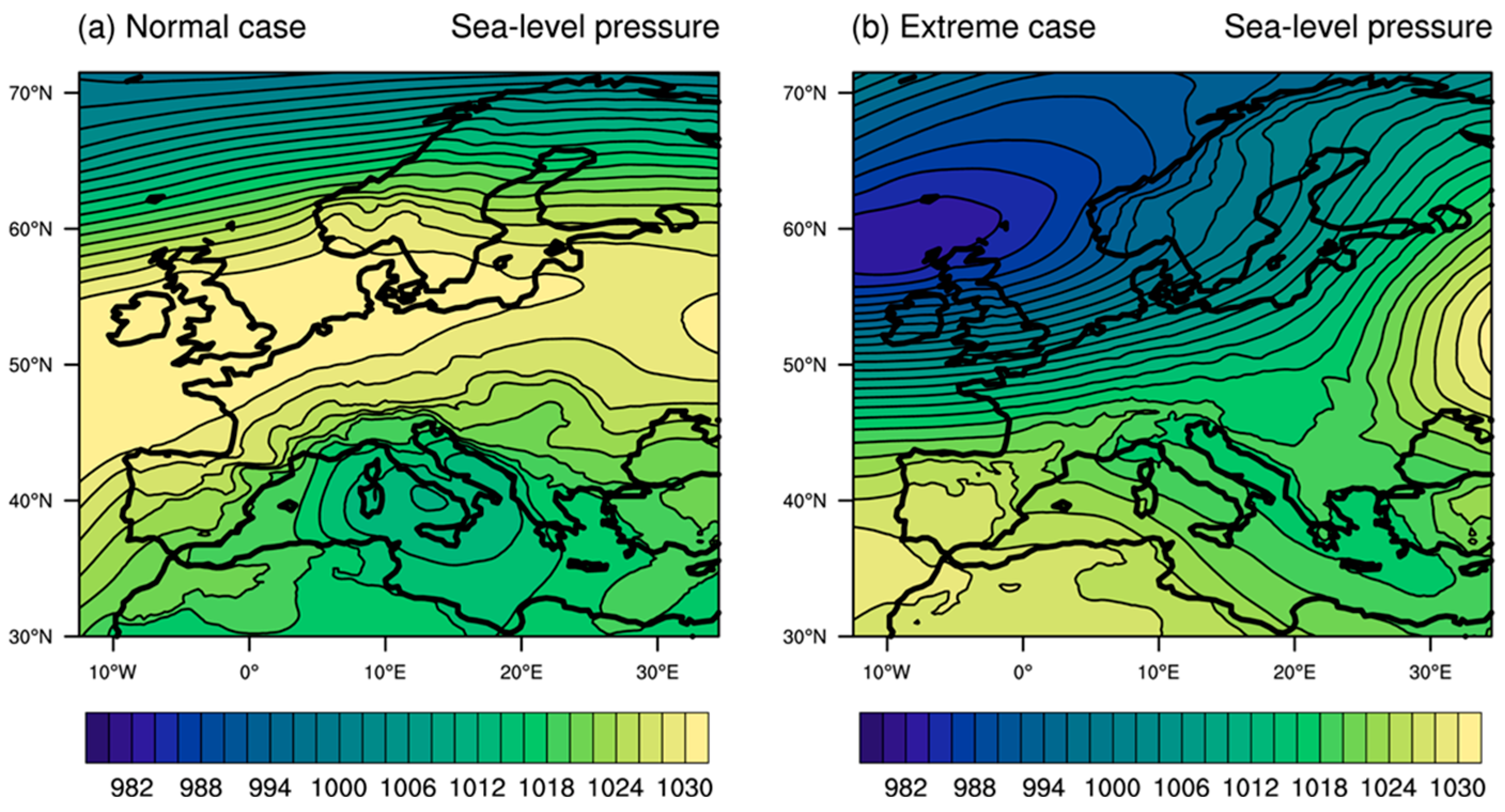
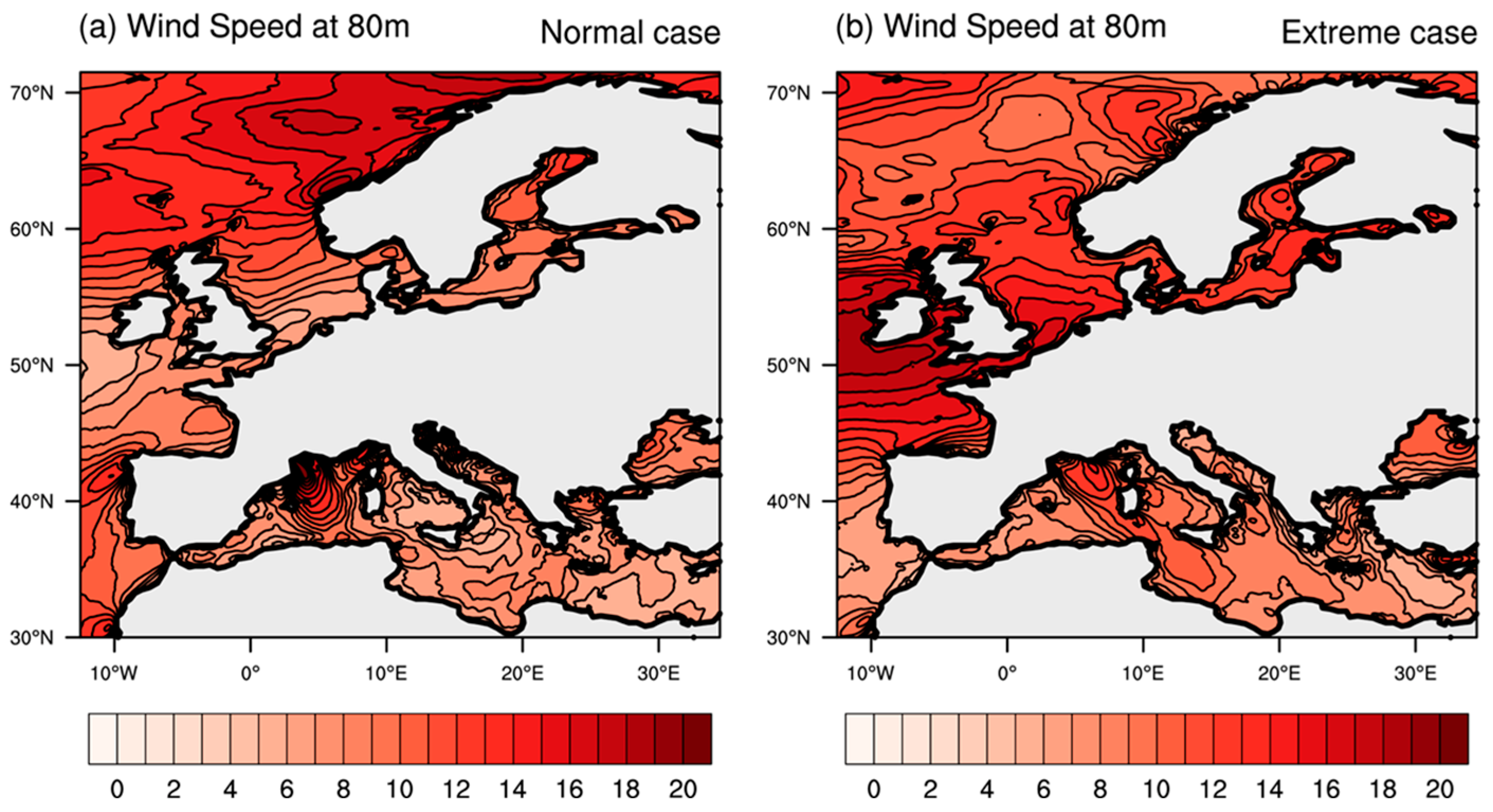
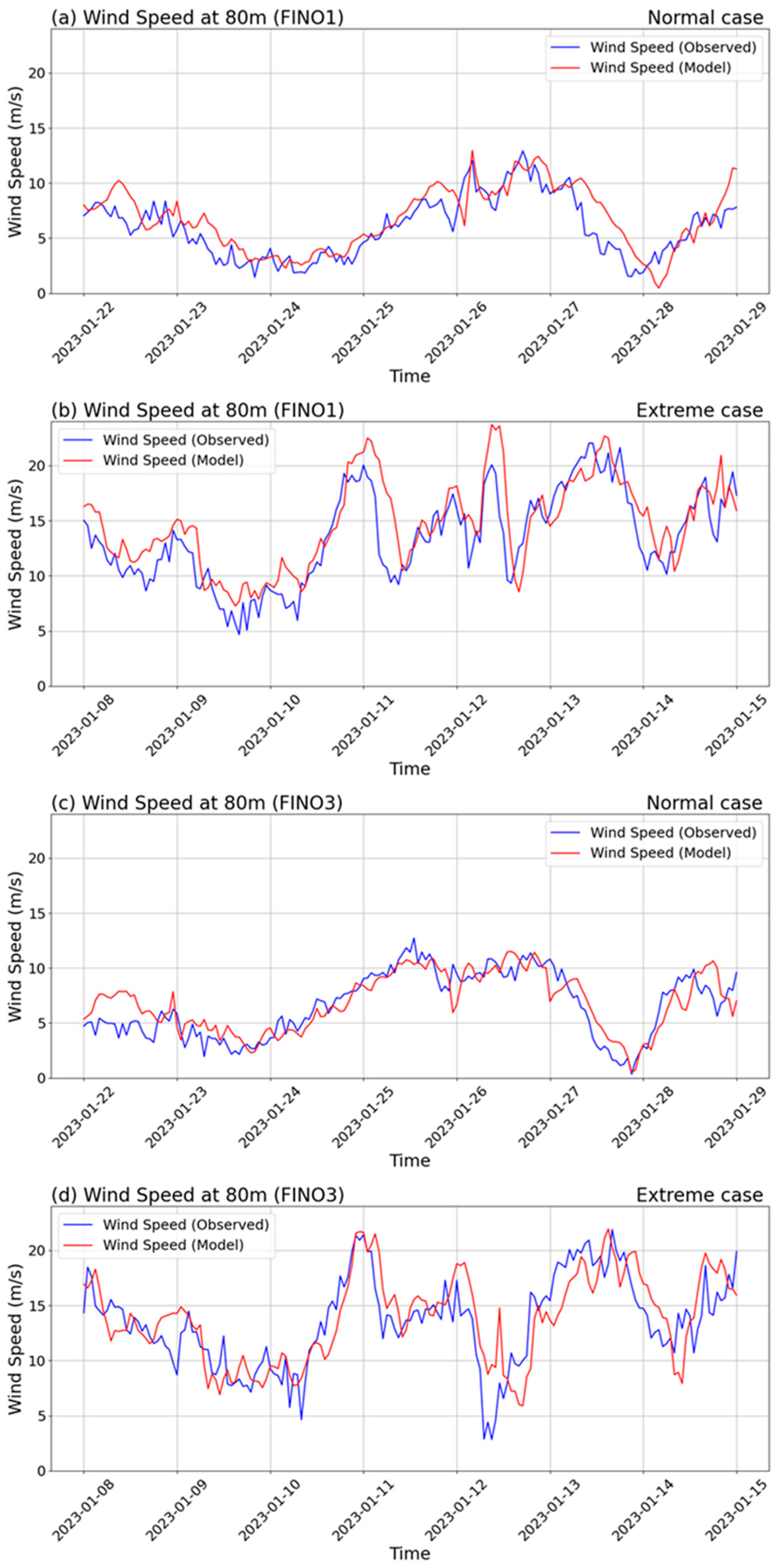
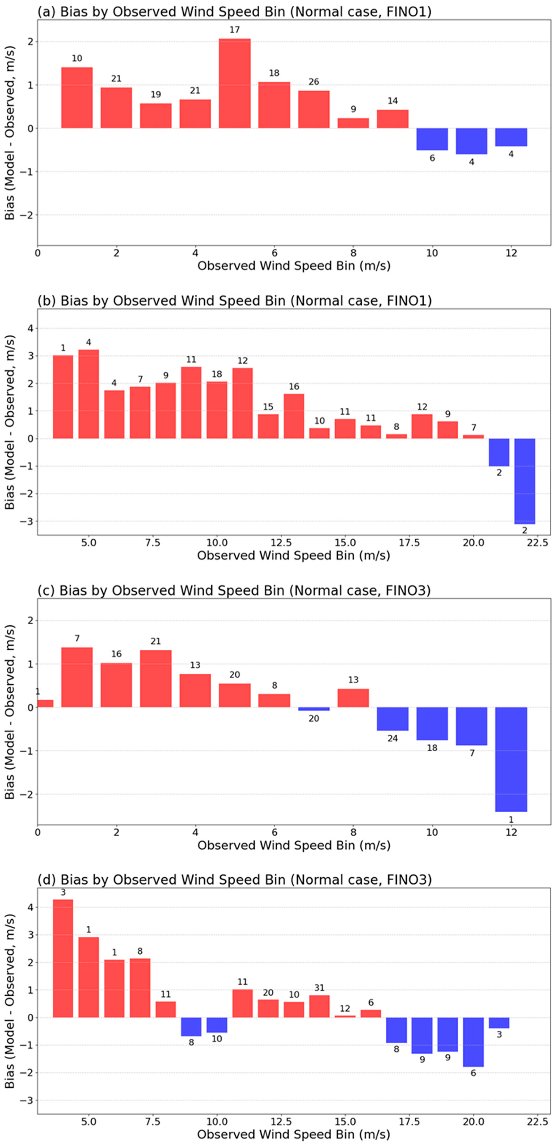
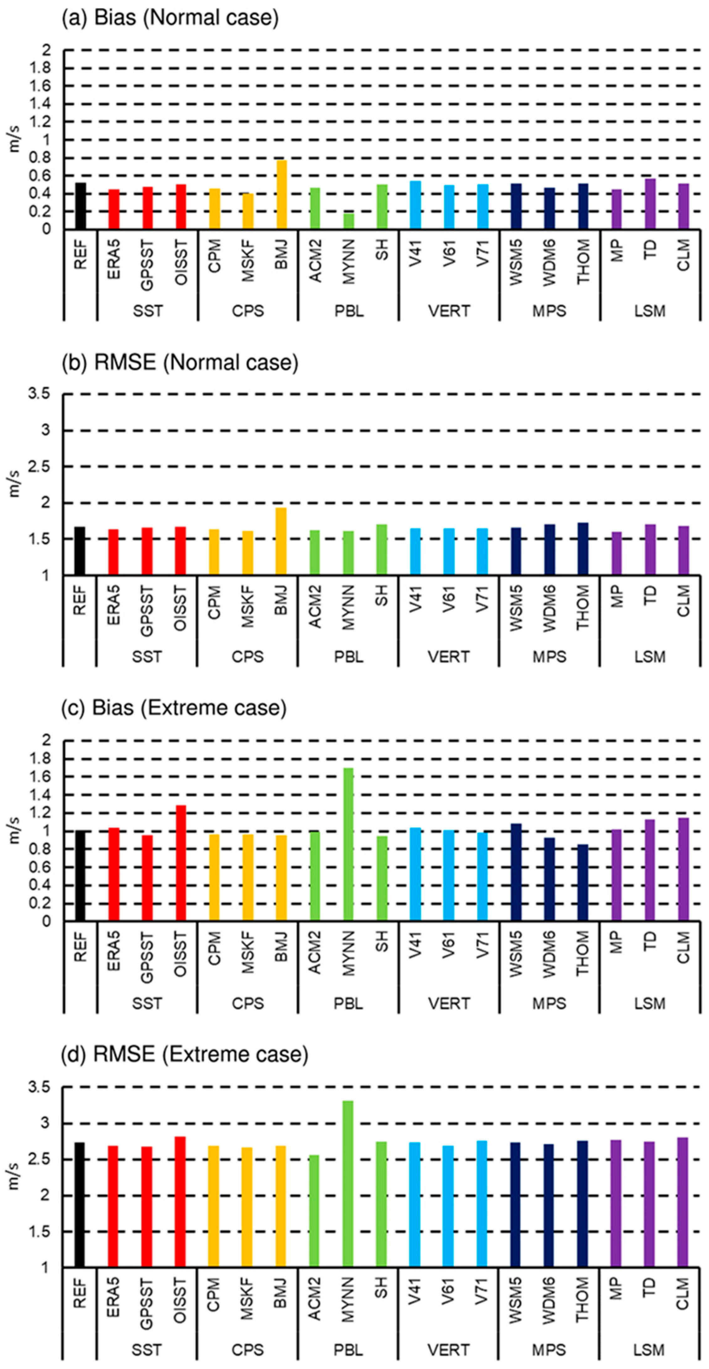
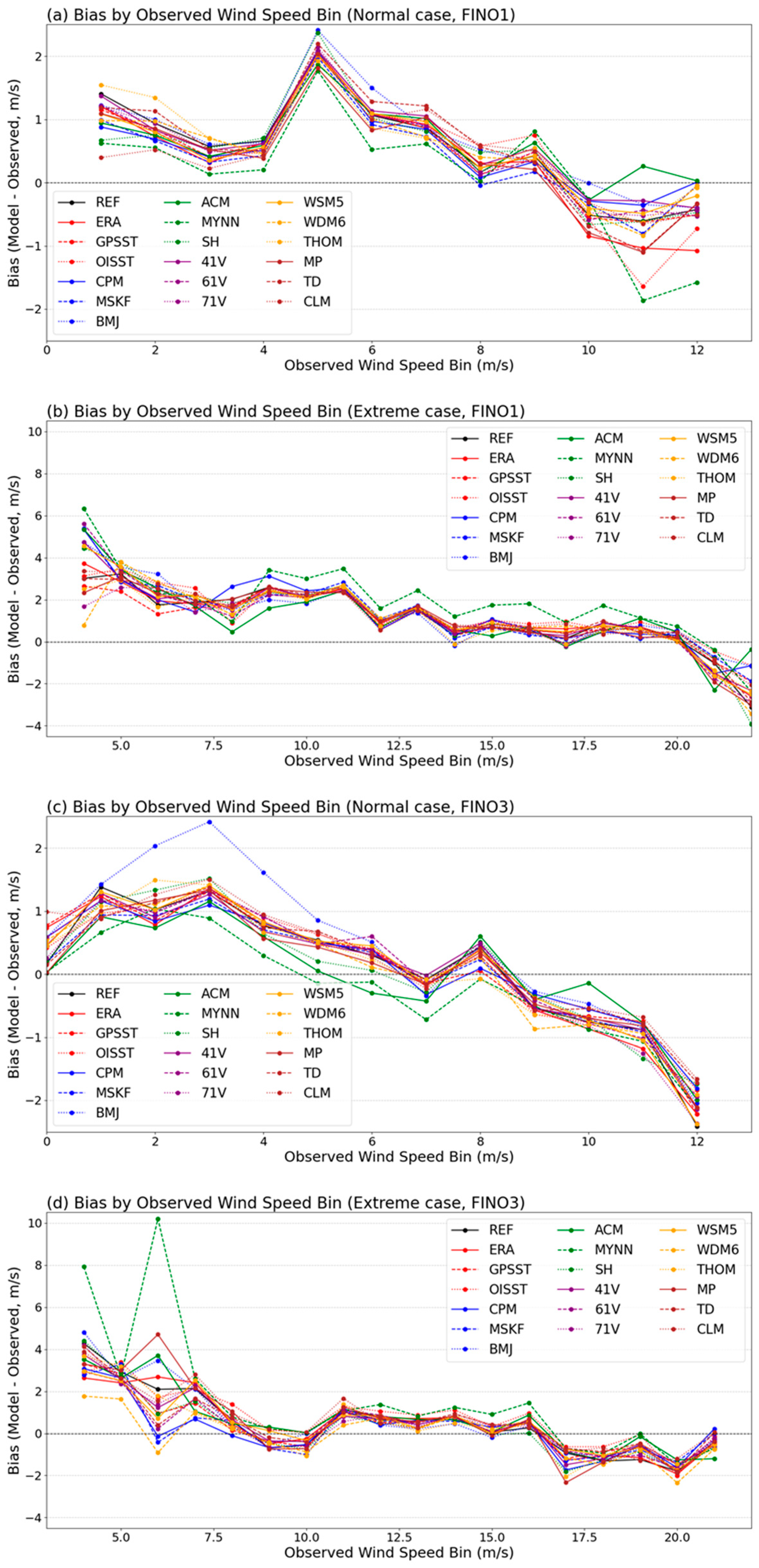
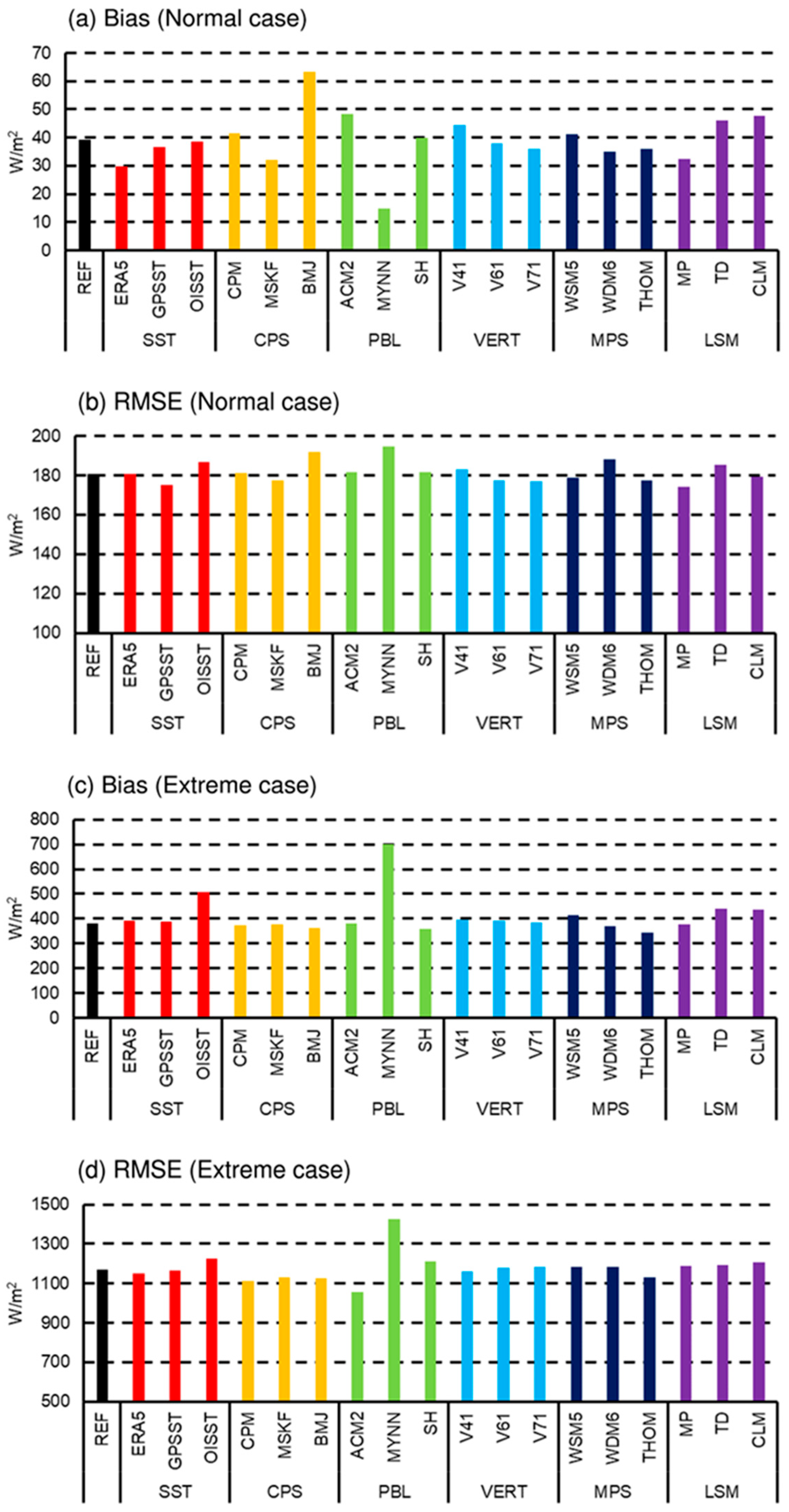
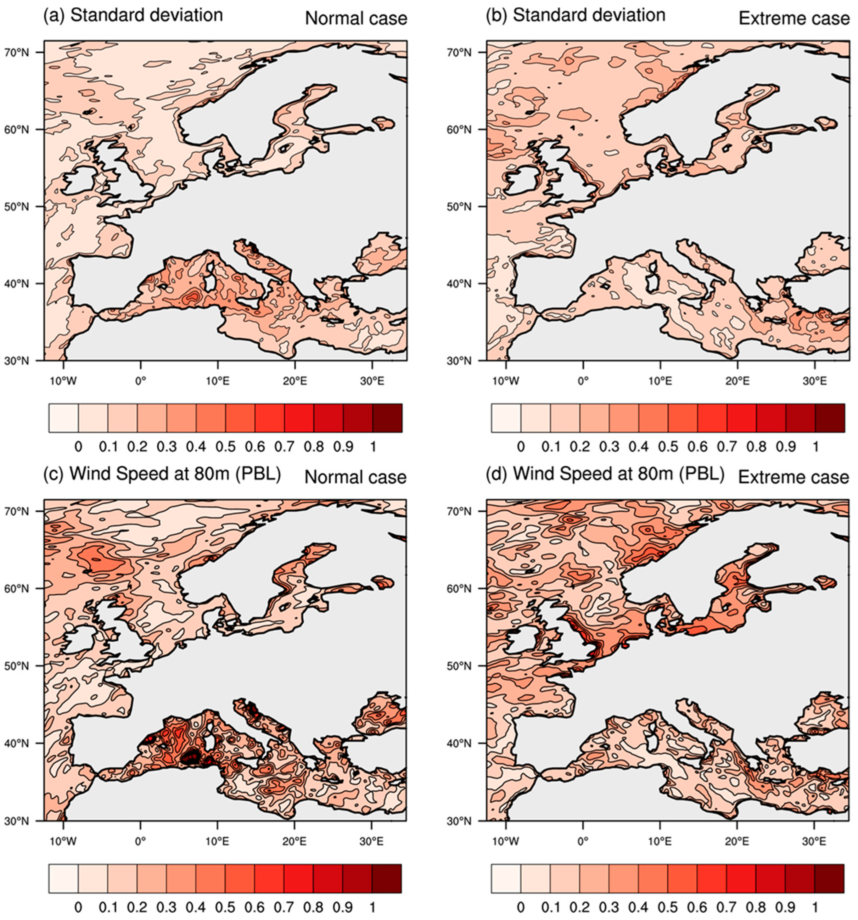
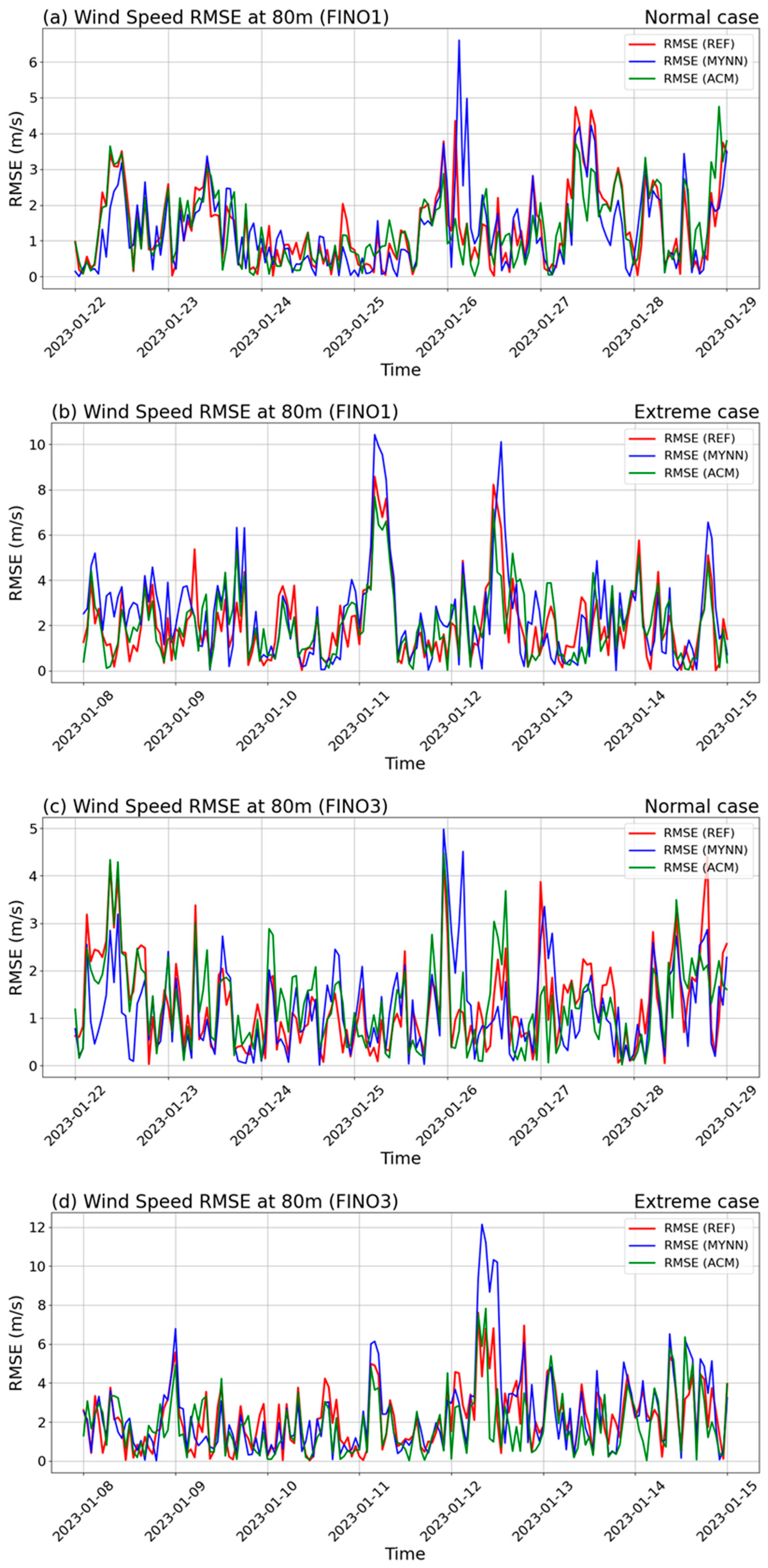
3.1. Model Performance Evaluation

This study focused on evaluating wind energy, emphasizing wind speeds at 80 m height, which corresponds to the hub height of wind turbines (Figure 3). Most offshore wind farms are located in the North Sea, Baltic Sea, and Irish Sea, regions known for their abundant wind resources and relatively stable conditions, leading to their suitability for offshore wind energy development [52]. In the normal case, wind speeds were relatively weak in these areas (approximately 7 m/s), whereas in the extreme case, strong winds were detected in regions where many wind farms are located. Near the Irish Sea, wind speeds exceeded an average of 20 m/s during the simulation period in extreme case, accompanied by intense rainfall due to the influence of a low-pressure system. In the areas where FINO platforms are located, wind speeds averaged around 7 m/s in the normal case, but almost doubled to 14 m/s in the extreme case.
To verify whether the REF experiment of the WRF model reasonably reproduced the large-scale environments, basic statistical metrics, including bias, Root Mean Square Difference (RMSD), and pattern correlation (PC), were examined (Table 3) [53]. PC is calculated by the Pearson product–moment coefficient of linear correlation at corresponding locations on two different maps. Although reanalysis data are not considered true values, these metrics allow for a quantitative assessment of how well the WRF model approximates the reanalysis data. The REF experiment simulated 500 hPa geopotential heights slightly higher than the reanalysis data, with an RMSD of approximately 13 m. The pattern correlation was very high, exceeding 0.99, primarily due to the application of spectral nudging. The bias was small for 850 hPa wind speeds, with an RMSD of approximately 2.3 m/s. However, the pattern correlation was relatively lower compared to geopotential height because spectral nudging was not applied in the low levels, resulting in more considerable differences from the reanalysis data. The results of the REF experiment showed that the two representative atmospheric variables showed no significant deviations from the reanalysis data, and the differences between cases were not notable.
Based on a comparison with FINO observation data, we evaluated how accurately the model results, forced by ERA5 reanalysis data, represent actual wind speeds and verified the reliability of the REF experiment. Due to many missing values in the FINO2 data during the simulation period, only FINO1 and FINO3 data were used for validation. As previously mentioned, the normal case had an average wind speed of approximately 7 m/s, which was about half that of the extreme case, with an average wind speed of 14 m/s (Figure 4). The REF experiment reasonably simulates wind speeds for the normal case, successfully capturing temporal variations with high accuracy (Figure 4a,c). However, significant errors occurred in simulating the sharp wind speed drop between January 27 and 28, particularly at FINO1. In the extreme case, wind speed changes were much more abrupt compared with the normal case, potentially resulting in larger model errors (Figure 4b,d). In addition, even though the two observation sites were close to each other (Figure 1), there were periods when wind speed variations observed opposing trends. Between January 12 and 13, wind speeds at FINO1 exhibited a sharp increase, while FINO3 showed a sharp decrease. Although wind speed tendencies during this period contrasted, the REF experiment adequately captured the overall increasing and decreasing trends, though with some errors.
The characteristics of model errors were examined by analyzing error tendencies in relation to the wind speed observed at FINO (Figure 5). The REF experiment overestimated wind speeds compared to observations on average (approximately 0.54 and 0.82 m/s in normal and extreme cases, respectively). The REF experiment produced significant overestimations in areas with weak winds, leading to substantial errors. Conversely, the model underestimated wind speeds in regions with strong winds, resulting in large errors. These patterns were consistent across both the normal and extreme cases, confirming that errors intensified in extremely weak or strong winds. However, the overestimation in weak wind regions was much more apparent in the extreme case compared to the normal case. In the normal case, the average overestimation in wind speed was approximately 1 m/s. In contrast, in the extreme case, differences exceeding 2 m/s occurred frequently, and at FINO3, differences reached up to 4 m/s. In addition to physical schemes, improvements in initial conditions, data assimilation, and numerical configurations may also help enhance simulation accuracy.

3.2. Sensitivity Experiments

Various experiments were conducted to evaluate the sensitivity of the wind speed performance to different physical processes. This study analyzed how 80 m wind speeds are simulated by modifying parameterization schemes that represent key physical processes, such as SST data, CPS, PBL, VERT, MPS, and LSM. The selected datasets and schemes were based on physical processes and datasets commonly employed in previous studies [14,32,41,54,55]. Details of the sensitivity experiments conducted for each scheme and data are provided in Table 2. To quantitatively assess the model’s errors, bias and Root Mean Square Error (RMSE) were calculated to evaluate the overestimation or underestimation compared to observations. As shown in the previous figure, the REF experiment overestimated wind speeds, with the overestimation being approximately twice as large in the extreme case. The model overestimated wind speeds compared to observations in all sensitivity experiments (approximately 0.2–0.8 m/s and 0.8–1.7 m/s in normal and extreme cases, respectively), including the REF experiment, and the overestimation was notably more pronounced in the extreme case (Figure 6). Based on the bias, the MYNN PBL scheme showed the best performance in the normal case; however, it exhibited the most considerable bias in the extreme case, indicating that consistent results were not simulated across different experiments (Figure 6a,c). In the extreme case, the MPS THOM scheme demonstrated the best performance in bias, followed by the MPS WDM6 scheme, which also realistically simulated wind speeds. The MPS can significantly influence near-surface wind simulations under extreme conditions accompanied by precipitation. Furthermore, a more considerable deviation between experiments was simulated compared to the normal case.
For RMSE in the normal case, most schemes produced similar errors, except for the CPS BMJ scheme, which showed larger discrepancies. In contrast, the extreme case exhibited a relatively larger deviation, with the PBL MYNN scheme showing the highest errors, while the ACM2 scheme achieved the best performance. The ACM2 scheme, as the second version of the Asymmetric Convective Model, employs a hybrid approach that considers both non-local mixing and local mixing, enabling it to simulate vertical turbulent flow and mixing within the atmospheric boundary layer [56,57]. Recent studies have suggested that ACM2’s hybrid approach performs well under event-driven unstable atmospheric conditions, such as extreme precipitation events [58]. RMSE values were also much higher in the extreme case than in the normal case, with more significant differences between experiments reproduced in the extreme case, particularly for the PBL schemes.
We have conducted an additional analysis examining the bias as a function of observed wind speed to evaluate model performance across the full spectrum of observed wind speeds in all sensitivity experiments (Figure 7). Each line represents a different sensitivity experiment, and we have grouped them by physics category (e.g., PBL, MPS, CPS) using a consistent color scheme for clarity. The results, consistent with those in Figure 6, reveal that biases become significantly more pronounced under extreme wind conditions. Across both the normal and extreme cases, and at both FINO1 and FINO3 sites, all sensitivity experiments exhibit a systematic overestimation at low observed wind speeds and an underestimation at high observed wind speeds. Furthermore, we found that the spread in bias among different experiments increases at both ends of the wind speed spectrum. This strengthens the importance of carefully evaluating model performance in these regimes, near the cut-in and cut-off thresholds, as they are particularly critical for wind energy applications.
Since a nonlinear relationship exists between wind speed and wind power density (WPD), evaluating wind speed accuracy alone is insufficient to fully assess wind energy potential. WPD is influenced by both wind speed and air density and is defined by the following equation [59,60]:
W P D = 1 2 ρ v 3
where ρ represents air density (kg m−3), and v denotes wind speed (m/s). This equation indicates that WPD is proportional to the cube of wind speed, meaning that any errors in wind speed are significantly amplified in WPD calculations. Consequently, even minor wind speed errors can lead to substantial deviations in WPD, especially under extreme wind conditions, directly affecting wind farm energy production estimates and design processes. To evaluate the sensitivity of WPD, we analyzed variations in different physical parameterization schemes and input datasets. In the normal case, the sensitivity of WPD was relatively high for the CPS and PBL schemes, exhibiting similar trends to wind speed simulations. Additionally, experiments with a larger number of vertical levels resulted in lower errors (Figure 8a,b). In the extreme case, the MYNN PBL scheme exhibited the poorest performance, whereas the ACM2 scheme demonstrated the highest accuracy, consistent with wind speed results (Figure 8c,d). This finding highlights the significant impact of PBL parameterization schemes on WPD reliability under extreme weather conditions. The hybrid turbulence mixing approach of the ACM2 scheme appears to yield more stable results in extreme wind conditions. Furthermore, bias and RMSE of WPD revealed substantially larger errors in the extreme case compared to the normal case, with even more pronounced discrepancies than those observed in wind speed errors (Figure 6). These results suggest that while improvements in physical parameterizations may have limited effects under normal wind conditions, enhancing model performance under extreme wind conditions can significantly improve the accuracy of wind energy potential assessments. Therefore, optimizing physical parameterization schemes for extreme weather conditions is crucial for ensuring the safe operation of wind energy systems and enhancing the reliability of energy production.
The performance and sensitivity analyses discussed above were based on FINO observation points located in offshore wind farm areas. Additionally, the spatial distribution of wind speed standard deviation was investigated across the entire European domain using the results from all sensitivity experiments (Figure 9a,b). The standard deviation of wind speeds simulated in all experiments was calculated for each grid point. This approach allowed for a visual assessment of how deviations vary between cases and regions. In the offshore regions near the FINO observations, where offshore wind farms are densely located, the standard deviation in the extreme case was larger than in the normal case. Over the entire domain, the sensitivity experiments revealed that wind speed deviations were most significantly affected by PBL schemes (Figure 9c,d), with LSMs also having a notable impact in land regions. These results highlight the large influence of PBL schemes on simulated wind speed variability and demonstrate that model errors tend to be larger under extreme wind conditions.

4. Summary and Conclusions

This study utilized a high-resolution WRF model with a high resolution of 6 km to simulate and identify systematic errors in the WRF model configuration associated with offshore wind speeds over Europe, using ERA5 as initial and lateral boundary conditions. The REF experiment served as a control, employing datasets and physical parameterization schemes widely used in previous studies. Case studies were selected from January 2023, with the normal case representing relatively weak winds and the extreme case a period of strong winds, both in regions with a high concentration of offshore wind farms. Cases were identified based on sea-level pressure patterns. Observational data were obtained from FINO observation platforms located in the North Sea and Baltic Sea (FINO1 and FINO3). Each simulation covered 8 days, with the first day used as a spin-up period and the remaining 7 days analyzed.
The REF experiments, designed to evaluate the community WRF set-up, showed that the model realistically captured synoptic conditions at 500 hPa and 850 hPa, as well as local temporal variations in wind speeds at 80 m compared to observations during the analysis period. However, it struggled to simulate rapidly changing wind speeds, particularly in the extreme case. In this case, average wind speeds were approximately twice as high as those in the normal case, resulting in larger variability and amplified errors. The analysis of model errors based on observed wind speed showed that the model tended to overestimate in weak wind conditions (approximately 1 m/s) and underestimate in strong wind conditions (approximately 3 m/s), with the most pronounced errors occurring in extremely weak or strong wind periods.
The sensitivity experiments were conducted by modifying one parameter at a time from the REF experiment for the SST dataset, CPS, BPL, MPS, LSM schemes, and vertical levels. All sensitivity experiments, including the REF experiment, overestimated wind speeds compared to FINO observations, with more significant results in the extreme case. The model’s performance differed between cases, with the ACM2 PBL scheme simulating the best results in the extreme case, and no notable differences among the experiments were observed under normal conditions. When examining the spatial standard deviation within the European domain, simulations indicated relatively larger deviations over land compared to offshore regions, attributed to factors such as surface roughness. Moreover, PBL schemes, which simulate turbulent processes in the lower atmosphere and directly influence near-surface winds, exhibited significant variability across the domain.
This study conducted WRF experiments with a horizontal resolution of 6 km. This resolution may be insufficient for evaluating wind speeds at wind farms, particularly in complex mountainous regions, coastal areas, or densely concentrated wind farm regions. The primary evaluation areas in this study were offshore regions, such as those around FINO. As a result, the limitations of the resolution have a comparatively minor influence in this context. Furthermore, the model was run for 8 days (7 days analysis) for each of the two cases, which does not account for seasonal characteristics and limits the sample size, making it difficult to perform extensive analysis. To mitigate the limitation of the short simulation period, we have examined the time series of simulation errors in PBL schemes (REF (YSU), MYNN, and ACM2 schemes) to investigate whether the anomalous performance is due to continuous errors or isolated events. Our findings show that large errors for the MYNN scheme tend to occur during periods when the observed wind speeds change rapidly, particularly in the extreme case (Figure 4 and Figure 10). During these periods of abrupt changes, all schemes, including REF (YSU), MYNN, and ACM2, exhibited increased errors. However, while the ACM2 and REF (YSU) schemes simulated relatively smaller errors, the MYNN scheme showed significantly larger errors at both FINO1 and FINO3 sites, especially during periods of rapid fluctuations in wind speed. This result aligns with previous findings [46,61], which indicated that the MYNN scheme would underperform in offshore environments. However, since short-term simulations still present challenges, future research will involve long-term simulations exceeding one year using the ACM2 PBL scheme, which demonstrated high performance in this study. Simulations will be conducted over two domains with 6 km and 2 km resolutions. The 2 km domain will focus on a smaller region of interest, rather than the entire European domain, to consider computational resources and allow for more detailed analysis in interest areas.
Evaluating all combinations of physical parameterizations provided by the WRF model is computationally prohibitive. Therefore, this study fixed the REF experiment configuration and varied only the target physical processes for sensitivity experiments. Additionally, differences in development levels of individual physical parameterizations could not be fully considered. Experiments were designed based on physical processes and datasets frequently employed in previous studies to address these limitations.
In near-surface wind simulations, distinguishing between weak and extreme winds is critical because they are directly related to wind power efficiency and safety. The results of this study confirm that errors and sensitivity to physical parameterizations can vary depending on the cases analyzed. Future long-term simulations aim to provide more reliable conclusions. Furthermore, sensitivity experiments emphasized the particularly significant role of PBL schemes in near-surface wind simulations. Finally, the relatively large errors observed in the extreme case highlight the need for continued research and improvement in simulating extreme wind conditions.

Author Contributions

This research was supported by all authors. Conceptualization, M.L. and J.-Y.K.; methodology, M.L., D.O. and J.-Y.K.; software, M.L. and D.O.; validation, M.L.; formal analysis, M.L.; investigation, M.L.; resources, C.K.K.; data curation, M.L., D.O. and J.-Y.K.; writing—original draft preparation, M.L.; writing—review and editing, M.L., D.O. and J.-Y.K.; visualization, M.L.; supervision, J.-Y.K. and C.K.K.; project administration, J.-Y.K. and, C.K.K.; funding acquisition, J.-Y.K. and C.K.K. All authors have read and agreed to the published version of the manuscript.

Funding

This work was supported by the Korea Institute of Energy Technology Evaluation and Planning (KETEP) and the Ministry of Trade, Industry and Energy (MOTIE) of the Republic of Korea (No. RS-2023-00301792), and conducted under the framework of the research and development program of the Korea Institute of Energy Research (C5-2422).

Institutional Review Board Statement

Not applicable.

Informed Consent Statement

Not applicable.

Data Availability Statement

The data supporting the findings of this study are available from the corresponding author upon reasonable request.

Acknowledgments

The authors would like to express their gratitude to the Korea Institute of Energy Research (KIER) for their support in conducting this research.

Conflicts of Interest

The authors declare no conflicts of interest.

References

  1. DeCastro, M.; Salvador, S.; Gómez-Gesteira, M.; Costoya, X.; Carvalho, D.; Sanz-Larruga, F.J.; Gimeno, L. Europe, China and the United States: Three different approaches to the development of offshore wind energy. Renew. Sustain. Energy Rev. 2019, 109, 55–70. [Google Scholar] [CrossRef]
  2. Europe, W. Wind Energy in Europe: 2023 Statistics and the Outlook for 2024–2030. Available online: https://windeurope.org/intelligence-platform (accessed on 21 March 2024).
  3. Panciatici, P.; Leader, W.; Pache, C.; Maeght, R.; Weber, R. E-Highway 2050 Modular Development Plan of the Pan-European Transmission System 2050; European Commission: Brussels, Belgium, 2016. [Google Scholar]
  4. Wang, J.; Qin, S.; Jin, S.; Wu, J. Estimation methods review and analysis of offshore extreme wind speeds and wind energy resources. Renew. Sustain. Energy Rev. 2015, 42, 26–42. [Google Scholar] [CrossRef]
  5. Wang, K.; Hansen, M.O.L.; Moan, T. Dynamic analysis of a floating vertical axis wind turbine under emergency shutdown using hydrodynamic brake. Energy Procedia 2014, 53, 56–69. [Google Scholar] [CrossRef]
  6. Chen, X.; Li, C.; Tang, J. Structural integrity of wind turbines impacted by tropical cyclones: A case study from China. Proc. J. Phys. Conf. Ser. 2016, 753, 042003. [Google Scholar] [CrossRef]
  7. İlkiliç, C. Wind energy and assessment of wind energy potential in Turkey. Renew. Sustain. Energy Rev. 2012, 16, 1165–1173. [Google Scholar] [CrossRef]
  8. Dabbaghiyan, A.; Fazelpour, F.; Abnavi, M.D.; Rosen, M.A. Evaluation of wind energy potential in province of Bushehr, Iran. Renew. Sustain. Energy Rev. 2016, 55, 455–466. [Google Scholar] [CrossRef]
  9. Onea, F.; Deleanu, L.; Rusu, L.; Georgescu, C. Evaluation of the wind energy potential along the Mediterranean Sea coasts. Energy Explor. Exploit. 2016, 34, 766–792. [Google Scholar] [CrossRef]
  10. Moemken, J.; Reyers, M.; Feldmann, H.; Pinto, J.G. Future changes of wind speed and wind energy potentials in EURO-CORDEX ensemble simulations. J. Geophys. Res. Atmos. 2018, 123, 6373–6389. [Google Scholar] [CrossRef]
  11. Hannesdóttir, Á.; Kelly, M.; Dimitrov, N. Extreme wind fluctuations: Joint statistics, extreme turbulence, and impact on wind turbine loads. Wind Energy Sci. 2019, 4, 325–342. [Google Scholar] [CrossRef]
  12. Li, H.; Claremar, B.; Wu, L.; Hallgren, C.; Körnich, H.; Ivanell, S.; Sahlée, E. A sensitivity study of the WRF model in offshore wind modeling over the Baltic Sea. Geosci. Front. 2021, 12, 101229. [Google Scholar] [CrossRef]
  13. Vemuri, A.; Munters, W.; Buckingham, S.; Helsen, J.; Van Beeck, J. Modeling extreme weather events for offshore wind in the North Sea: A sensitivity analysis to physics parameterizations in WRF. Proc. J. Phys. Conf. Ser. 2022, 2265, 022014. [Google Scholar] [CrossRef]
  14. Carvalho, D.; Rocha, A.; Gómez-Gesteira, M.; Santos, C. A sensitivity study of the WRF model in wind simulation for an area of high wind energy. Environ. Model. Softw. 2012, 33, 23–34. [Google Scholar] [CrossRef]
  15. Davidson, M.R.; Millstein, D. Limitations of reanalysis data for wind power applications. Wind Energy 2022, 25, 1646–1653. [Google Scholar] [CrossRef]
  16. Gualtieri, G. Analysing the uncertainties of reanalysis data used for wind resource assessment: A critical review. Renew. Sustain. Energy Rev. 2022, 167, 112741. [Google Scholar] [CrossRef]
  17. Leiding, T.; Tinz, B.; Gates, L.; Rosenhagen, G.; Herklotz, K.; Senet, C. Standardisierung und Vergleichende Analyse der Meteorologischen FINO-Messdaten (FINO123): Forschungsvorhaben FINO-Wind: Abschlussbericht: 12/2012-04/2016; Deutscher Wetterdienst: Offenbach, Germany, 2016. [Google Scholar]
  18. Skamarock, W.C.; Klemp, J.B.; Dudhia, J.; Gill, D.O.; Barker, D.M.; Duda, M.G.; Huang, X.-Y.; Wang, W.; Powers, J.G. A description of the advanced research WRF version 3. NCAR Tech. Note 2008, 475, 10-5065. [Google Scholar]
  19. Hersbach, H.; Bell, B.; Berrisford, P.; Hirahara, S.; Horányi, A.; Muñoz-Sabater, J.; Nicolas, J.; Peubey, C.; Radu, R.; Schepers, D. The ERA5 global reanalysis. Q. J. R. Meteorol. Soc. 2020, 146, 1999–2049. [Google Scholar] [CrossRef]
  20. Giorgi, F.; Jones, C.; Asrar, G.R. Addressing climate information needs at the regional level: The CORDEX framework. World Meteorol. Organ. (WMO) Bull. 2009, 58, 175. [Google Scholar]
  21. Donlon, C.J.; Martin, M.; Stark, J.; Roberts-Jones, J.; Fiedler, E.; Wimmer, W. The operational sea surface temperature and sea ice analysis (OSTIA) system. Remote Sens. Environ. 2012, 116, 140–158. [Google Scholar] [CrossRef]
  22. Kain, J.S. The Kain–Fritsch convective parameterization: An update. J. Appl. Meteorol. 2004, 43, 170–181. [Google Scholar] [CrossRef]
  23. Hong, S.-Y.; Noh, Y.; Dudhia, J. A new vertical diffusion package with an explicit treatment of entrainment processes. Mon. Weather Rev. 2006, 134, 2318–2341. [Google Scholar] [CrossRef]
  24. Hong, S.Y. A new stable boundary-layer mixing scheme and its impact on the simulated East Asian summer monsoon. Q. J. R. Meteorol. Soc. 2010, 136, 1481–1496. [Google Scholar] [CrossRef]
  25. Hong, S.-Y.; Lim, J.-O.J. The WRF single-moment 6-class microphysics scheme (WSM6). Asia-Pac. J. Atmos. Sci. 2006, 42, 129–151. [Google Scholar]
  26. Ek, M.; Mitchell, K.; Lin, Y.; Rogers, E.; Grunmann, P.; Koren, V.; Gayno, G.; Tarpley, J. Implementation of Noah land surface model advances in the National Centers for Environmental Prediction operational mesoscale Eta model. J. Geophys. Res. Atmos. 2003, 108, 8851. [Google Scholar] [CrossRef]
  27. Jiménez, P.A.; Dudhia, J.; González-Rouco, J.F.; Navarro, J.; Montávez, J.P.; García-Bustamante, E. A revised scheme for the WRF surface layer formulation. Mon. Weather Rev. 2012, 140, 898–918. [Google Scholar] [CrossRef]
  28. Iacono, M.J.; Delamere, J.S.; Mlawer, E.J.; Shephard, M.W.; Clough, S.A.; Collins, W.D. Radiative forcing by long-lived greenhouse gases: Calculations with the AER radiative transfer models. J. Geophys. Res. Atmos. 2008, 113, D13103. [Google Scholar] [CrossRef]
  29. von Storch, H.; Langenberg, H.; Feser, F. A spectral nudging technique for dynamical downscaling purposes. Mon. Weather Rev. 2000, 128, 3664–3673. [Google Scholar] [CrossRef]
  30. Laurila, T.K.; Sinclair, V.A.; Gregow, H. Climatology, variability, and trends in near-surface wind speeds over the North Atlantic and Europe during 1979–2018 based on ERA5. Int. J. Clim. 2021, 41, 2253–2278. [Google Scholar] [CrossRef]
  31. Roberts, J.; Champion, A.; Dawkins, L.; Hodges, K.; Shaffrey, L.; Stephenson, D.; Stringer, M.; Thornton, H.; Youngman, B. The XWS open access catalogue of extreme European windstorms from 1979 to 2012. Nat. Hazards Earth Syst. Sci. 2014, 14, 2487–2501. [Google Scholar] [CrossRef]
  32. Witha, B.; Hahmann, A.N.; Sile, T.; Dörenkämper, M.; Ezber, Y.; Bustamante, E.G.; González-Rouco, J.F.; Leroy, G.; Navarro, J. Report on WRF Model Sensitivity Studies and Specifications for the Mesoscale Wind Atlas Production Runs: Deliverable D4. 3. 2019. Available online: https://backend.orbit.dtu.dk/ws/portalfiles/portal/180023688/2019_05_09_NEWA_D4_3_final.pdf (accessed on 29 March 2025).
  33. Bhattacharya, S. Civil engineering aspects of a wind farm and wind turbine structures. In Wind Energy Engineering; Elsevier: Amsterdam, The Netherlands, 2023; pp. 121–136. [Google Scholar]
  34. Small, R.J.; Xie, S.-P.; Wang, Y.; Esbensen, S.K.; Vickers, D. Numerical simulation of boundary layer structure and cross-equatorial flow in the eastern Pacific. J. Atmos. Sci. 2005, 62, 1812–1830. [Google Scholar] [CrossRef]
  35. Spall, M.A. Midlatitude wind stress–sea surface temperature coupling in the vicinity of oceanic fronts. J. Clim. 2007, 20, 3785–3801. [Google Scholar] [CrossRef]
  36. Lindzen, R.S.; Nigam, S. On the role of sea surface temperature gradients in forcing low-level winds and convergence in the tropics. J. Atmos. Sci. 1987, 44, 2418–2436. [Google Scholar] [CrossRef]
  37. Tompkins, A.M. On the relationship between tropical convection and sea surface temperature. J. Clim. 2001, 14, 633–637. [Google Scholar] [CrossRef]
  38. Lee, S.-H.; Lee, H.-W.; Kim, Y.-K.; Jeon, W.-B.; Choi, H.-J.; Kim, D.-H. Impact of continuously varied SST on land-sea breezes and ozone concentration over south-western coast of Korea. Atmos. Environ. 2011, 45, 6439–6450. [Google Scholar] [CrossRef]
  39. Ma, L.-M.; Tan, Z.-M. Improving the behavior of the cumulus parameterization for tropical cyclone prediction: Convection trigger. Atmos. Res. 2009, 92, 190–211. [Google Scholar] [CrossRef]
  40. Shepherd, T.J.; Walsh, K.J. Sensitivity of hurricane track to cumulus parameterization schemes in the WRF model for three intense tropical cyclones: Impact of convective asymmetry. Meteorol. Atmos. Phys. 2017, 129, 345–374. [Google Scholar] [CrossRef]
  41. Pradhan, P.; Liberato, M.L.; Ferreira, J.A.; Dasamsetti, S.; Rao, S.V.B. Characteristics of different convective parameterization schemes on the simulation of intensity and track of severe extratropical cyclones over North Atlantic. Atmos. Res. 2018, 199, 128–144. [Google Scholar] [CrossRef]
  42. Shen, W.; Song, J.; Liu, G.; Zhuang, Y.; Wang, Y.; Tang, J. The effect of convection scheme on tropical cyclones simulations over the CORDEX East Asia domain. Clim. Dyn. 2019, 52, 4695–4713. [Google Scholar] [CrossRef]
  43. Park, H.; Kim, G.; Cha, D.H.; Chang, E.C.; Kim, J.; Park, S.H.; Lee, D.K. Effect of a scale-aware convective parameterization scheme on the simulation of convective cells-related heavy rainfall in South Korea. J. Adv. Model. Earth Syst. 2022, 14, e2021MS002696. [Google Scholar] [CrossRef]
  44. Shin, H.H.; Hong, S.-Y. Intercomparison of planetary boundary-layer parametrizations in the WRF model for a single day from CASES-99. Bound.-Layer Meteorol. 2011, 139, 261–281. [Google Scholar] [CrossRef]
  45. Hu, X.M.; Klein, P.M.; Xue, M. Evaluation of the updated YSU planetary boundary layer scheme within WRF for wind resource and air quality assessments. J. Geophys. Res. Atmos. 2013, 118, 10490–10505. [Google Scholar] [CrossRef]
  46. Carvalho, D.; Rocha, A.; Gómez-Gesteira, M.; Santos, C.S. Sensitivity of the WRF model wind simulation and wind energy production estimates to planetary boundary layer parameterizations for onshore and offshore areas in the Iberian Peninsula. Appl. Energy 2014, 135, 234–246. [Google Scholar] [CrossRef]
  47. Khain, A.; Lynn, B.; Shpund, J. High resolution WRF simulations of Hurricane Irene: Sensitivity to aerosols and choice of microphysical schemes. Atmos. Res. 2016, 167, 129–145. [Google Scholar] [CrossRef]
  48. Park, J.; Cha, D.H.; Lee, M.K.; Moon, J.; Hahm, S.J.; Noh, K.; Chan, J.C.; Bell, M. Impact of cloud microphysics schemes on tropical cyclone forecast over the western North Pacific. J. Geophys. Res. Atmos. 2020, 125, e2019JD032288. [Google Scholar] [CrossRef]
  49. Lee, C.B.; Kim, J.-C.; Belorid, M.; Zhao, P. Performance evaluation of four different land surface models in WRF. Asian J. Atmos. Environ. 2016, 10, 42–50. [Google Scholar] [CrossRef]
  50. Wu, Z.; Jiang, C.; Deng, B.; Chen, J.; Liu, X. Sensitivity of WRF simulated typhoon track and intensity over the South China Sea to horizontal and vertical resolutions. Acta Oceanol. Sin. 2019, 38, 74–83. [Google Scholar] [CrossRef]
  51. Ma, Z.; Fei, J.; Huang, X.; Cheng, X. Sensitivity of tropical cyclone intensity and structure to vertical resolution in WRF. Asia-Pac. J. Atmos. Sci. 2012, 48, 67–81. [Google Scholar] [CrossRef]
  52. Deveci, M.; Özcan, E.; John, R. Offshore wind farms: A fuzzy approach to site selection in a black sea region. In Proceedings of the 2020 IEEE Texas Power and Energy Conference (TPEC), College Station, TX, USA, 6–7 February 2020; pp. 1–6. [Google Scholar]
  53. Kim, J.Y.; Kim, D.Y.; Oh, J.H. Projected changes in wind speed over the Republic of Korea under A1B climate change scenario. Int. J. Climatol. 2014, 34, 1346. [Google Scholar] [CrossRef]
  54. Fernández-González, S.; Martín, M.L.; García-Ortega, E.; Merino, A.; Lorenzana, J.; Sánchez, J.L.; Valero, F.; Rodrigo, J.S. Sensitivity analysis of the WRF model: Wind-resource assessment for complex terrain. J. Appl. Meteorol. Climatol. 2018, 57, 733–753. [Google Scholar] [CrossRef]
  55. Song, H.-J.; Sohn, B.-J. An evaluation of WRF microphysics schemes for simulating the warm-type heavy rain over the Korean peninsula. Asia-Pac. J. Atmos. Sci. 2018, 54, 225–236. [Google Scholar] [CrossRef]
  56. Pleim, J.E. A combined local and nonlocal closure model for the atmospheric boundary layer. Part I: Model description and testing. J. Appl. Meteorol. Climatol. 2007, 46, 1383–1395. [Google Scholar] [CrossRef]
  57. Pleim, J.E. A combined local and nonlocal closure model for the atmospheric boundary layer. Part II: Application and evaluation in a mesoscale meteorological model. J. Appl. Meteorol. Climatol. 2007, 46, 1396–1409. [Google Scholar] [CrossRef]
  58. Wasson, G.; Panda, S. Sensitivity of PBL parameterization schemes in simulating lightning and thunderstorm using WRF-ELEC model. Clim. Dyn. 2024, 62, 3799–3821. [Google Scholar] [CrossRef]
  59. Manyonge, A.W.; Ochieng, R.; Onyango, F.; Shichikha, J. Mathematical modelling of wind turbine in a wind energy conversion system: Power coefficient analysis. Appl. Math. Sci. 2012, 6, 4527–4536. [Google Scholar]
  60. Chen, L.; Li, G.; Zhang, F.; Wang, C. Simulation uncertainty of near-surface wind caused by boundary layer parameterization over the complex terrain. Front. Energy Res. 2020, 8, 554544. [Google Scholar] [CrossRef]
  61. Bodini, N.; Optis, M.; Redfern, S.; Rosencrans, D.; Rybchuk, A.; Lundquist, J.K.; Pronk, V.; Castagneri, S.; Purkayastha, A.; Draxl, C. The 2023 National Offshore Wind data set (NOW-23). Earth Syst. Sci. Data Discuss. 2023, 2023, 1–57. [Google Scholar]
Figure 1. (a) Model domain and topography used in this study. The red dashed box represents the analysis area. (b) Locations of the FINO observation platforms (FINO1 and FINO3) are indicated by colored dots in both (a) and (b).
Atmosphere 16 00665 g001
Figure 2. Sea-level pressure for the (a) normal case and (b) extreme case, averaged over the 7-day analysis period. The analysis period for the normal case is from 22 January 2023/00 UTC to 29 January 2023/00 UTC, and the analysis period for the extreme case is from 8 January 2023/00 UTC to 15 January 2023/00 UTC.
Atmosphere 16 00665 g002
Figure 3. Spatial distribution of 80 m wind speeds (m/s) in the reference experiment for the (a) normal case and (b) extreme case during the analysis period. Contour interval is 2 m/s.
Atmosphere 16 00665 g003
Figure 4. Time series of 80 m wind speed from the reference experiment and FINO observations. The blue line represents observed wind speeds from FINO, and the red line indicates the simulated wind speeds from the reference experiment. Figures (a,c) correspond to the normal case, and panels (b,d) correspond to the extreme case at FINO1 and FINO3, respectively.
Atmosphere 16 00665 g004
Figure 5. The bias of wind speed based on observed wind speed bins for the (a,c) normal case, and (b,d) extreme case. Red bars represent overestimation (positive bias), and blue bars represent underestimation (negative bias). Each bar corresponds to a 1 m/s observed wind speed interval. Data are shown for FINO1 in (a,b) and FINO3 in (c,d). The number above or below each bar indicates the count of data points within each bin.
Atmosphere 16 00665 g005
Figure 6. (a,c) Bias, and (b,d) RMSE of 80 m wind speed for the normal and extreme cases, respectively. The average values from FINO1 and FINO3 observations are used for comparison. Each bar represents the results for different sensitivity experiments among SST, CPS, PBL, VERT, MPS, and LSM configurations.
Atmosphere 16 00665 g006
Figure 7. Bias based on observed wind speed bins for (a,c) normal case, and (b,d) extreme case. Each line represents a sensitivity experiment, grouped by physics scheme (color) and differentiated by line style. Positive values indicate overestimation, while negative values indicate underestimation. Bin intervals are 1 m s−1.
Atmosphere 16 00665 g007
Figure 8. Same as Figure 6, but for wind power density (W m−2).
Atmosphere 16 00665 g008
Figure 9. Spatial distribution of the standard deviation of 80 m wind speed among all sensitivity experiments for the normal (a) and extreme (b) cases, with (c,d) representing the standard deviation calculated solely from the PBL schemes for each case.
Atmosphere 16 00665 g009
Figure 10. Time series of RMSE for 80 m wind speed between WRF simulations and FINO observations for the REF (YSU, red lines), MYNN (blue lines), and ACM2 (green lines) PBL schemes. Figures (a,c) represent the normal case, and figures (b,d) indicate the extreme case, for the FINO1 and FINO3 sites, respectively.
Atmosphere 16 00665 g010
Table 1. Reference (REF) configuration of the WRF model used in this study, including details on the model version, initial and lateral boundary conditions, resolution, and physical parameterization schemes.
ModelWRF v4.5.1
Domain (grid points)Europe (837 × 879)
(latitudinal and longitudinal grid points, respectively)
Initial and boundary forcingERA5 reanalysis (0.25° × 0.25°)
Horizontal resolution6 km grid spacing
Vertical resolution51 levels
Time step30 s
Simulation period8 days
(1 day spin-up + 7 days analysis)
SST datasetOSTIA (6 km resolution)
ConvectionKain–Fritsch
Planetary boundary layerYSU
MicrophysicsWSM6
Land-surfaceUnified Noah
Surface layerRevised MM5
Short, longwave radiationRRTMG
Table 2. Configuration of sensitivity experiments for each physical process and dataset.
Sensitivity Experiment
SST
(Sea surface temperature)
ERA5 (0.25° × 0.25°)
(ECMWF Reanalysis v5)
GPSST (1 km resolution)
(Geo-Polar Blended Sea Surface Temperature)
OISST (25 km resolution)
(Optimum Interpolation Sea Surface Temperature)
CPS
(Cumulus parameterization scheme)
CPM (Convection-permitting model)
MSKF (Multi-Scale Kain–Fritsch)
BMJ (Bett-Miller–Janjic)
PBL
(Planetary boundary layer)
ACM2 (Asymmetrical Convective Model 2)
MYNN (Mellor-Yamada-Nakanishi-Niino)
SH (Shin and Hong)
VERT
(Vertical levels)
V41 (41 vertical levels)
V61 (61 vertical levels)
V71 (71 vertical levels)
MPS
(Microphysics scheme)
WSM5 (WRF Single-Moment 5-class)
WDM6 (WRF Single-Moment 5-class)
THOM (Thompson)
LSM
(Land surface model)
MP (Noah-MP)
TD (Thermal Diffusion)
CLM (Community Land Model version 4)
Table 3. Bias, RMSD, and pattern correlation (PC) of 500 hPa geopotential height and 850 hPa wind speed between the reference experiment and ERA5 reanalysis data for the normal and extreme case.
VariablesCaseBiasRMSDPC
500 hPa geopotential height (m)Normal6.55213.1650.997
Extreme6.93912.5140.999
850 hPa
wind speed (m/s)
Normal0.0542.2980.920
Extreme0.0392.3800.918
Disclaimer/Publisher’s Note: The statements, opinions and data contained in all publications are solely those of the individual author(s) and contributor(s) and not of MDPI and/or the editor(s). MDPI and/or the editor(s) disclaim responsibility for any injury to people or property resulting from any ideas, methods, instructions or products referred to in the content.

