The Effects of Nonplanar Cloud Top on Lightning Optical Observations from Space-Based Instruments

Abstract

Satellite optical observations of lightning are influenced by a variety of factors. Studying these factors can provide valuable reference information for applications such as lightning parameter inversion. However, due to the variability of natural factors and the high cost of field observations, research requiring controlled variables often relies heavily on effective simulation models. To this end, we applied our developed optical transmission model for lightning, which can simultaneously account for the spatiotemporal characteristics of lightning sources and observation angles, as well as inhomogeneous and irregular cloud environments, to analyze an unexplained hypothesis from previous studies—that non-planar cloud tops may also be an influencing factor. Our analysis confirms that non-planar cloud tops are indeed an important factor that must be considered, especially under smaller or larger observation angles. In the simulation results, undulations caused an energy increase of up to 43.19% at a 0° observation angle, while at a 60° observation angle, the undulations resulted in an additional attenuation of approximately 17.5%.

1. Introduction

As lightning emits intense optical radiation that can be observed from space, several satellite-based instruments for detecting lightning optical emissions have been commissioned over the past decades, including the Optical Transient Detector (OTD), Lightning Imaging Sensor (LIS), Geostationary Lightning Mapper (GLM), and Lightning Mapping Imager (LMI) [1,2,3,4,5]. Most of these instruments rely on cameras with wavelength filters centered around 777.4 nm, which is a strong emission line of lightning. However, due to the influence of different lightning sources and clouds on the propagation path, the observed lightning radiation results vary greatly. In order to better explain these observations and use them, it is necessary to establish a model for simulation to identify and analyze possible influencing factors. Early models include those developed by Thomson, Koshak et al., and Light et al. [6,7,8]. The models using the Monte Carlo method among them has been further improved and applied afterwards.

The simple models proposed in early research have already been able to explain some basic principles. Light et al. [8] confirmed that the shape of the cloud and position of the lightning event in the cloud (rather than the extent or motion of the source) are the primary factors that determine the distribution of photons escaping to space. For example, the shape of the cloud and the location of the lightning event within the cloud may affect the distribution of photons escaping into space. When lightning occurs at low altitude within the cloud, the energy propagating to the cloud top is significantly reduced, making the lightning less likely to be observed. However, these models can only consider simple cloud scenes and cannot generate the simulated observed images.

As observational data accumulates, some phenomena that cannot be explained by previous models have emerged [9,10,11,12,13,14] (e.g., the appearance of dim “holes” within a large, illuminated region), which has prompted researchers to develop more comprehensive models that can consider more factors. Peterson [15] uses the Monte Carlo Atmospheric Radiative Transfer Simulator (MCARaTS) to conduct the research and confirms that diffuse reflections of nearby cloud faces are an important factor that determines how the radiance measured from above is spatially distributed across the scene. Brunner and Bitzer [16] were the first to add inhomogeneous environments adapted from Weather Research and Forecasting (WRF) simulation to the previous computational model. They studied the effects of inhomogeneous scattering environments and source geometry on the lightning optical radiation reaching cloud tops, finding that the gradient effect in the mean free path (MFP) profile also has a significant impact on the optical radiation of lightning at cloud tops. They hypothesized that a non-planar cloud top would also have a significant impact, which is a key aspect of this research.

In previous studies, the clouds employed for models were typically constructed by assembling simple geometric shapes, which clearly lack the ability to represent large-scale, randomly fluctuating cloud tops. To more effectively account for the complex and undulating structures of real-world cloud tops in simulations, we referred to existing lightning optical transmission models and established a model suitable for the 777.4 nm band. This model is capable of flexibly constructing cloud-top structures while simultaneously considering the spatiotemporal characteristics of lightning sources, observation angles, and cloud inhomogeneity. Subsequently, we used this model to simulate lightning optical observations under various conditions, including different cloud-top structures, cloud environments, observation angles, and horizontal extents of clouds. The simulation results were then analyzed to evaluate the influence of non-planar cloud top on lightning observation outcomes.

2. Methods

Based on the models proposed by Thomson and Krider, Light et al., and Luque [6,8,17], we developed a new model for lightning light radiation in the 777.4 nm band. This model accounts for complex three-dimensional cloud structures, varying observation angles, and the spatiotemporal characteristics of lightning sources, and it is capable of generating simulated observation images. Due to the low absorption rate in the 777.4 nm band, the effect of absorption is ignored in the model. When simulating the geostationary satellite observation results, the detector is located at an altitude of 35,786 km above the ground, with a spatial resolution of 4 km × 4 km, and the total size of the simulated image is 2400 pixels × 2400 pixels.

2.1. Simulation Process

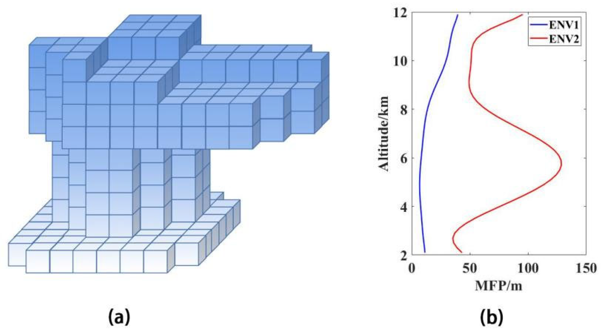
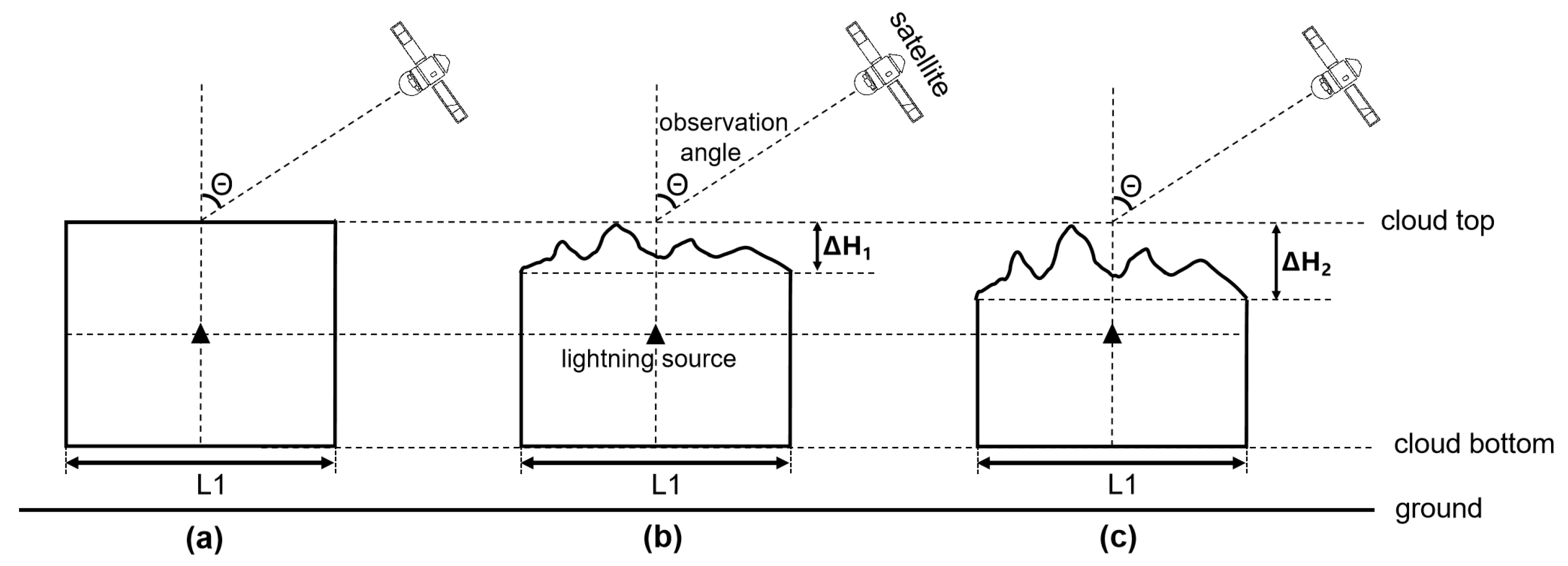
During the simulation, the photons are emitted isotropically from the lightning source and propagate independently. Each photon is tracked as it undergoes multiple scattering until it leaves the simulation domain, its energy drops below the threshold, or its number of scattering events reaches the maximum (set to 10⁶ in this study according to Luque [17]).

In order to determine the new position of photons after scattering, it is necessary to obtain the scattering direction and propagation distance, which depends on the type of scattering. In our model, we consider two different types of scattering: Mie scattering [18] and Rayleigh scattering [19]. When a photon is inside the cloud, it undergoes Mie scattering; otherwise, it undergoes Rayleigh scattering.

When photons undergo Mie scattering, the scattering direction is determined by the Henyey–Greenstein phase function [6,20]:

$$p\left(\mu \right)={\displaystyle \frac{1-g^2}{{\left(1+g^2-2g\mu \right)}^{3/2}}}$$

(1)

where g is known as the “asymmetry parameter” which is the average of the cosine of the scattering angle.

The traveling distance of each step is a randomized distribution of the MFP, now

$$s=-\ln \left(r\right)·\mathsf{\Lambda }$$

(2)

where r is an independent random variable uniformly distributed in the interval [0,1) and Λ represents the MFP, which depends on the particle number concentration (N) and mean radius (r) in the area.

When photons undergo Rayleigh scattering, we obtain scattering direction and the collision rate V_R using the same method as Luque [17]. The traveling distance of each step is then determined as follows:

$$s=-\ln \left(r\right)/V_R$$

(3)

The initial energy of each photon is 1 unit and only decreases after a Mie scattering event. The reduction ratio is determined by the w₀ (referred to as the single-scattering albedo, and a value of 0.99998 is used). The value of w₀ was chosen for two primary reasons. First, because according to the findings of Bohren [21], this value is most appropriate for the cloud environment and radiation wavelength considered in this study. Second, it was selected based on previous studies of lightning optical radiation simulations [6,16], which employed the same value and achieved reasonable results. If the energy of the ith scattering, w_i, is lower than the default value (0.01 in this article), the Russian roulette method [22] is used to determine whether to terminate the simulation of this photon or not.

Furthermore, since we are simulating the optical radiation received by a detector far away from the source, the probability of each simulated photon reaching the detector along a given scattering direction is negligible. To achieve reliable observation results with a limited number of simulated photons, we also employ the local estimation method described by Luque [17].

2.2. Cloud Settings

The different shapes of clouds are approximated through the combination of 3D grids with a side length of 200 m, as shown in Figure 1a. The choice to use 3D grids to form clouds was made because it is easier to reproduce undulating cloud tops. In this study, we used two ranges rectangular clouds with 10 km and 20 km. Both clouds’ base heights were set at 2 km, and the maximum cloud top height was 12 km.

The environment in a 3D cubic grid is all the same. By assigning different MFP values to these cubic grids, an inhomogeneous cloud can be formed. A total of three different environments (HM, ENV1VC, ENV2VC) were constructed in this study. In the HM environment, all cubic grids have a constant MFP value (~15.91 m), which is the same as that used by Thomson and Krider, Light et al., and Brunner [6,8,16]. In ENV1VC and ENV2VC, the MFP only changes vertically, meaning that the MFP of the cubic grids of the same height in the layer remains consistent with the assigned value. The vertical changes in MFP are shown in Figure 1b (refer to the WRF simulation results of Brunner [16]).

2.3. Lightning Source

In order to simulate the result of realistic lightning, the model needs to consider the spatiotemporal characteristics of lightning. This is because lightning propagates along an extended channel at a limited speed, and the emitted energy also changes over time. In this study, a combination of regularly spaced point sources is used to represent the channel geometry. Each point source is isotropic and shares the total number of photons initially set. By sequentially activating these point sources over time, the extension of lightning channels at different speeds with time can be simulated. The activation time of each point source is determined by adding the distance between the current point source and the previous one divided by the propagation speed to the activation time of the previous point source. The activation time for the first point source is zero.

Then, the time at which the optical radiation reaches the detector is determined by summing the initial time and the propagation time of each photon. The initial time of the photon is determined based on the activation time of the point source that emitted the photon and the emission power equation adapted from Light [8], while the propagation time is obtained by dividing the total propagation distance by the speed of light. The propagation distance of a photon is defined as the sum of its total scattering distance and the distance from the cloud to the detector.

2.4. Observation Angle

In our model, different real-world observation angles are represented by adjusting the prescribed zenith and azimuth angles. Based on these specified angles, along with the Earth’s radius and the cloud base height, the results of the simulation are transformed into the coordinate system of the imaging plane. This transformation uses geometric projection relationships and local estimation methods [17], allowing us to obtain simulated observations corresponding to the specified viewing angle. Due to the high computational cost of optical simulations using the Monte Carlo method—particularly for large-scale scenarios—it is impractical to simulate all possible cases. Therefore, selecting representative scenarios is a more reasonable approach. To simplify the analysis of observation angle variations, only the zenith angle was adjusted to represent changes in viewing geometry. Considering that the typical zenith angle range for observations from geostationary satellites is approximately 0° to 60°, we selected three representative angles (0°, 30°, and 60°) for simulation and analysis in this research. These angles have also been commonly used in previous studies.

3. Results

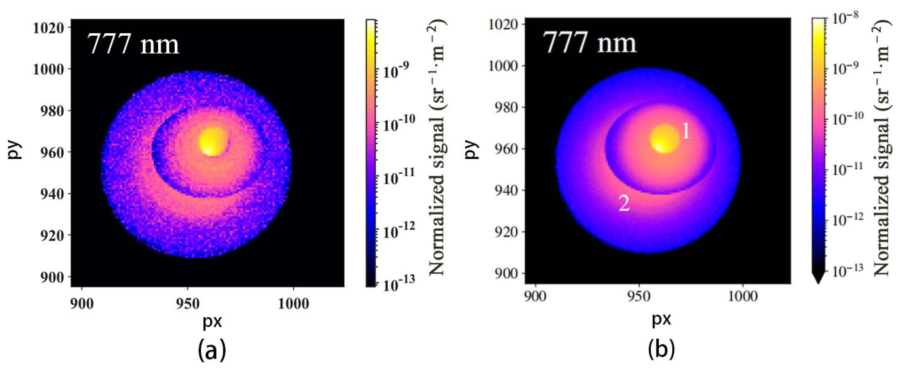
3.1. Model Verification

Firstly, we compared the result simulated by our model with the result obtained by Luque [17] at the 777.4 nm wavelength to validate the effectiveness of our model. The results are shown in Figure 2. Luque approximated a typical convective thunderstorm shape in his simulation by combining simple geometric shapes and adding a depression at the center. His simulated results align with the observation highlighted by Peterson [11]: “Quite often, the standout features of a lightning flash are depressions in the cloud geometry”. Our results are generally consistent with Luque’s in terms of optical radiation energy distribution, with the brightest region located in the same area and the maximum optical radiation energy being nearly identical. The slight differences between the results of the two models may stem from variations in the methods used to construct the cloud layer and the lightning source. This demonstrates that our model is also suitable for lightning optical radiation simulations and can be used to study relevant influencing factors and patterns.

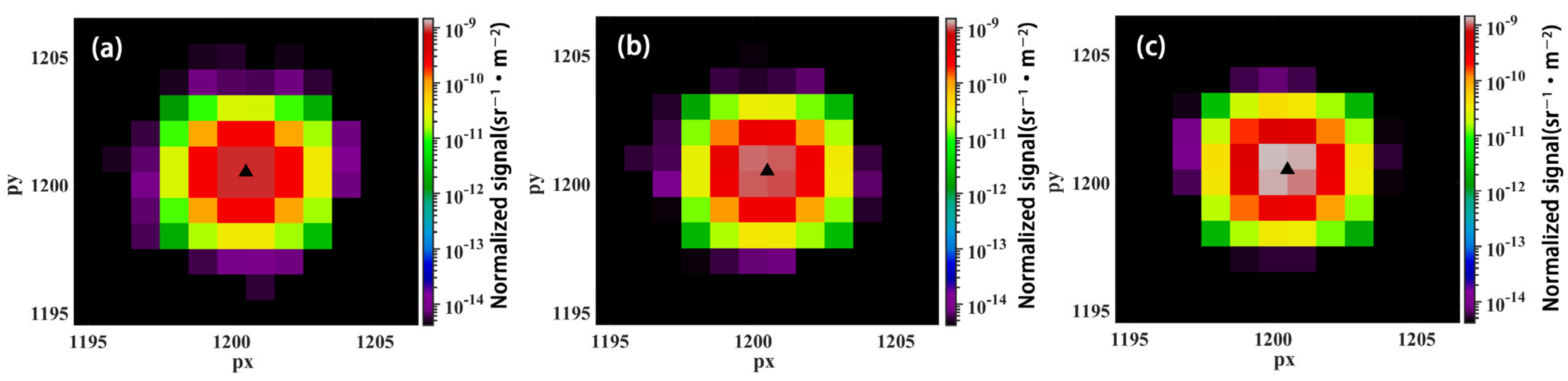
3.2. The Effect of Nonplanar Cloud Top

Based on the cubic cloud, we constructed three types of clouds with different degrees of undulating tops, as shown in Figure 3. These are called flat cloud top, Undulation 1, and Undulation 2, respectively. The altitude of the ground is 0 km and the altitude of the cloud bottom and cloud top are 2 km and 12 km, respectively. The position of the light source, unless otherwise specified, is located at 7 km altitude and at the horizontal center. The cloud top height is randomly reduced within a certain range from the maximum height of 12 km at 200 m horizontal intervals. The variation ranges for the flat cloud top, Undulation 1, and Undulation 2 are 0 m, 400 m, and 800 m, respectively. L1 represents the horizontal extent of the cloud, which is 10 km or 20 km in this study. For simplicity, in the following sections, they will be referred to as 10 km clouds and 20 km clouds. A larger horizontal extent of the cloud means a greater distance from the source to the cloud’s side. Here, we simulated the results under three environments (HM, ENV1VC, and ENV2VC) and three typical angles (0°, 30°, and 60°). The results of the total observed radiation energy under the various conditions mentioned in this study can be found in Supplementary Table S1.

The simulation results indicate that at smaller observation angles, when the maximum cloud thickness is the same, the total optical radiation energy observed by the instrument increases as the cloud top undulation increases, especially in the region where the lightning source is located. Figure 4 and Figure 5 clearly show, from left to right, that at a 0° observation angle, under the same cloud horizontal size and inhomogeneous environment, the distribution of observed radiation energy changes significantly with increasing undulation, and the brightness in the central region increases notably. In the case of Undulation 2, the largest optical energy in the central region and the overall optical energy was observed. In the ENV1VC environment, for clouds with a 10 km horizontal extent, the observed total energy increased by 13.33% and 43.77% for Undulation 1 and Undulation 2, respectively, compared to the flat cloud top. For clouds with a 20 km horizontal extent, the increases were 15.63% and 43.19%, respectively. This trend was also observed in the other two environments. The increase is influenced, on the one hand, by the fact that for clouds with the same maximum thickness, those with larger undulations tend to have a smaller total optical thickness. On the other hand, it is related to the gradient of the mean free path (MFP) in the observation direction, which was considered an important factor in Brunner’s study [16]. When modifying the extent of cloud-top undulations, it inevitably alters the overall MFP gradient.

However, when the observation angle increases beyond a certain threshold, the increase in cloud-top undulations leads to a greater attenuation of the total optical radiation energy observed by the instrument. At an observation angle of 60 degrees, the total energy observed in cloud layers with horizontal extents of 10 km and 20 km all decrease further as the undulations increase, across different environmental conditions. Figure 6 and Figure 7 show the simulation results for two cloud sizes at a 60° observation angle under the ENV1VC environment. It can be seen that as the undulation increases, the energy observed in the higher brightness regions decreases significantly compared to the flat cloud top, even for Undulation 1 with relatively low undulation. For clouds with a 10 km horizontal extent, the observed total energy decreased by 15.62% and 22.39% for Undulation 1 and Undulation 2, respectively, compared to the flat cloud top, while for clouds with a 20 km horizontal extent, the decreases were 27.28% and 39.51%, respectively. Additionally, we compared the energy decay ratios of different cloud tops relative to a flat top at a 0° observation angle for a 60° observation angle. For all environments, the decay ratios showed an increasing trend. In clouds with two different horizontal extents (10 km/20 km) and the ENV1VC environment, by comparing the energy corresponding to flat-top clouds at 0° and 60° observation angles, we found that the attenuation caused purely by the increase in observation angle was 28.72% and 55.73%, respectively. However, in Undulation 1, these decay rates increased to 39.85% and 67.8%, while in Undulation 2, the decay rates were 44.68% and 73.22%, respectively. Clearly, at sufficiently large observation angles, cloud-top undulations induce additional attenuation beyond the decay caused by the increased observation angle, and this attenuation increases with the degree of undulation.

Figure 8 shows the energy attenuation rates relative to a flat cloud top at a 0° observation angle for different cloud tops at observation angles of 30° and 60°, under the same environmental conditions. It can be observed that, at an observation angle of 60°, the undulating cloud tops consistently result in greater attenuation, with the attenuation increasing as the degree of undulation increases. Furthermore, compared to clouds at 10 km altitude, clouds at 20 km exhibit more significant attenuation due to the increased cloud volume, which further increases the optical thickness from the light source to the cloud side. At larger observation angles, the additional attenuation caused by cloud-top undulations may be attributed to changes in the mean free path (MFP) gradient and overall optical thickness, leading to an increase in radiated energy in the cloud-top direction, while radiation in other directions decreases. However, at larger observation angles, most of the radiated energy in the cloud-top direction is not detected by the instruments. On the other hand, radiation may also encounter greater obstruction from the undulating cloud-top boundary during its journey to the detector. It is also worth noting that at the 30° observation angle, the effects do not exhibit a uniform increase or decrease, nor do they become more pronounced as the degree of undulation increases, as observed at 0° and 60°. This indicates that the final effect of cloud-top undulations is closely related to the observation angle. As the observation angle increases, cloud-top undulations cause greater attenuation, eventually surpassing the enhancement effect observed at smaller angles. When the observation angle is sufficiently large or small, the environment no longer influences the attenuation increase resulting from increased undulation. For certain environments at a 30° observation angle, the enhancement effect brought by undulations remains relatively noticeable, leading to a situation where larger undulations result in lower attenuation rates compared to smaller undulations.

4. Conclusions and Discussion

In this study, we developed a model that simultaneously considers undulated cloud tops, inhomogeneous environments, the spatiotemporal characteristics of lightning sources, and different observation angles. The model was then used to explore the factors influencing the measurement results of lightning optical radiation. We found that undulated cloud tops are also a significant factor influencing the observation results of lightning optical radiation, particularly at smaller or larger observation angles. The influence of undulations varies with the observation angle. At a 0° observation angle, larger undulations enhance the observed total optical radiation energy, with a maximum increase of 43.19% in the simulated results. This increase is due not only to the reduced optical thickness between the light source and the detector, but also to further changes in the vertical gradient of the mean free path (MFP) caused by the undulations. As the observation angle increases, undulations tend to cause greater attenuation of the total observed energy. For a cloud with a horizontal extent of 20 km in the ENV1VC environment, the attenuation rate of the total observed energy at a 60° observation angle under Undulation 2, relative to the flat cloud top with a 0° observation angle, is 73.22%, whereas it is only 55.73% under flat cloud tops. The additional attenuation of approximately 17.5% is clearly attributed to the undulating cloud tops. Clearly, the impact of cloud-top undulations exhibits a dual effect depending on the observation angle; at smaller observation angles, the enhancement effect far outweighs the attenuation, while at larger observation angles, the opposite is true. Considering that cloud top height is also a type of data collected by satellites, this allows us to consider cloud top height data for corrections when applying lightning optical radiation observation data, resulting in more accurate results.

In our study, as well as in previous research, the combined influence of various factors—including cloud morphology, cloud environment, and the lightning source itself—leads to nonlinear effects. For instance, lightning sources of the same intensity may produce significantly different distributions and magnitudes of optical energy at the observation instrument. This nonlinearity makes it challenging to directly infer lightning source characteristics solely from observational data. Given the complex and variable nature of these influencing factors, simulation studies that allow controlled manipulation of conditions are more suitable for identifying the key contributors to observed phenomena, rather than for directly establishing inversion-ready empirical relationships. Once the dominant factors are identified, they can be incorporated into potential application scenarios (e.g., lightning intensity retrieval) to improve accuracy. With the advancement of artificial intelligence, it becomes increasingly feasible to use large volumes of observational data associated with these influencing factors determined by simulation to train AI models that can effectively infer the desired parameters, making tasks such as lightning source inversion more efficient and practical.

When simulating with the model established using the Monte Carlo method and producing image results, an unavoidable issue is the lengthy computation time. A feasible method to reduce computation time is to set a height threshold, as proposed by Luque [17], ignoring the radiative contribution of photons below this height. However, there is no clear reference for what this height should be. Setting it too high would cause the model to overlook significant low-altitude radiation, leading to inaccurate results, especially at larger observation angles. Therefore, we believe that using better computational techniques, such as cluster computing, might be a more effective solution.

References

1. Boccippio, D.J.; Koshak, W.; Blakeslee, R.; Driscoll, K.; Mach, D.; Buechler, D.; Boeck, W.; Christian, H.J.; Goodman, S.J. The Optical Transient Detector (OTD): Instrument characteristics and cross-sensor validation. J. Atmos. Ocean. Technol. 2000, 17, 441–458. [Google Scholar] [CrossRef]
2. Blakeslee, R.J.; Lang, T.J.; Koshak, W.J.; Buechler, D.; Gatlin, P.; Mach, D.M.; Stano, G.T.; Virts, K.S.; Walker, T.D.; Cecil, D.J.; et al. Three years of the lightning imaging sensor onboard the international space station: Expanded global coverage and enhanced applications. J. Geophys. Res. Atmos. 2020, 125, e2020JD032918. [Google Scholar] [CrossRef]
3. Goodman, S.J.; Blakeslee, R.J.; Koshak, W.J.; Mach, D.; Bailey, J.; Buechler, D.; Carey, L.; Schultz, C.; Bateman, M.; McCaul, E.; et al. The GOES-R geostationary lightning mapper (GLM). Atmos. Res. 2013, 125, 34–49. [Google Scholar] [CrossRef]
4. Rudlosky, S.D.; Goodman, S.J.; Virts, K.S.; Bruning, E.C. Initial geostationary lightning mapper observations. Geophys. Res. Lett. 2019, 46, 1097–1104. [Google Scholar] [CrossRef]
5. Yang, J.; Zhang, Z.; Wei, C.; Lu, F.; Guo, Q. Introducing the new generation of Chinese geostationary weather satellites, Fengyun-4. Bull. Am. Meteorol. Soc. 2017, 98, 1637–1658. [Google Scholar] [CrossRef]
6. Thomson, L.W.; Krider, E.P. The effects of clouds on the light produced by lightning. J. Atmos. Sci. 1982, 39, 2051–2065. [Google Scholar] [CrossRef]
7. Koshak, W.J.; Solakiewicz, R.J.; Phanord, D.D.; Blakeslee, R.J. Diffusion model for lightning radiative transfer. J. Geophys. Res. Atmos. 1994, 99, 14361–14371. [Google Scholar] [CrossRef]
8. Light, T.E.; Suszcynsky, D.M.; Jacobson, A.R. Coincident radio frequency and optical emissions from lightning, observed with the FORTE satellite. J. Geophys. Res. Atmos. 2001, 106, 28223–28231. [Google Scholar] [CrossRef]
9. Curtis, N.; Carey, L.D.; Schultz, C. An analysis of the lightning jump algorithm using geostationary lightning mapper flashes. In Proceedings of the International Lightning Detection Conference (ILDC 2018), Fort Lauderdale, FL, USA, 12–15 March 2018. [Google Scholar]
10. Fuchs, B.R.; Rutledge, S.A. Investigation of lightning flash locations in isolated convection using LMA observations. J. Geophys. Res. Atmos. 2018, 123, 6158–6174. [Google Scholar] [CrossRef]
11. Peterson, M. Using lightning flashes to image thunderclouds. J. Geophys. Res. Atmos. 2019, 124, 10175–10185. [Google Scholar] [CrossRef] [PubMed]
12. Marchand, M.; Hilburn, K.; Miller, S.D. Geostationary Lightning Mapper and Earth Networks lightning detection over the contiguous United States and dependence on flash characteristics. J. Geophys. Res. Atmos. 2019, 124, 11552–11567. [Google Scholar] [CrossRef]
13. Peterson, M.; Liu, C. Characteristics of lightning flashes with exceptional illuminated areas, durations, and optical powers and surrounding storm properties in the tropics and inner subtropics. J. Geophys. Res. Atmos. 2013, 118, 11–727. [Google Scholar] [CrossRef]
14. Peterson, M. Holes in optical lightning flashes: Identifying poorly transmissive clouds in lightning imager data. Earth Space Sci. 2021, 8, e2020EA001294. [Google Scholar] [CrossRef]
15. Peterson, M. Modeling the transmission of optical lightning signals through complex 3-D cloud scenes. J. Geophys. Res. Atmos. 2020, 125, e2020JD033231. [Google Scholar] [CrossRef]
16. Brunner, K.N.; Bitzer, P.M. A first look at cloud inhomogeneity and its effect on lightning optical emission. Geophys. Res. Lett. 2020, 47, e2020GL087094. [Google Scholar] [CrossRef]
17. Luque, A.; Gordillo-Vázquez, F.J.; Li, D.; Malagón-Romero, A.; Pérez-Invernón, F.J.; Schmalzried, A.; Soler, S.; Chanrion, O.; Heumesser, M.; Neubert, T.; et al. Modeling lightning observations from space-based platforms (CloudScat. jl 1.0). Geosci. Model Dev. 2020, 13, 5549–5566. [Google Scholar] [CrossRef]
18. Wriedt, T. Mie theory: A review. In The Mie Theory: Basics and Applications; Springer: Berlin/Heidelberg, Germany, 2012; pp. 53–71. [Google Scholar]
19. Twersky, V. Rayleigh scattering. Appl. Opt. 1964, 3, 1150–1162. [Google Scholar] [CrossRef]
20. Danielson, R.E.; Moore, D.R.; Van de Hulst, H.C. The transfer of visible radiation through clouds. J. Atmos. Sci. 1969, 26, 1078–1087. [Google Scholar] [CrossRef]
21. Bohren, C.F.; Huffman, D.R. Absorption and scattering by a sphere. In Absorption and Scattering of Light by Small Particles; Wiley: Hoboken, NJ, USA, 1983; Volume 7, pp. 82–129. [Google Scholar]
22. Iwabuchi, H. Efficient Monte Carlo methods for radiative transfer modeling. J. Atmos. Sci. 2006, 63, 2324–2339. [Google Scholar] [CrossRef]
Figure 1. Description of how the three-dimensional cloud shapes were established and the cloud environments used in the research. (a) A random shape of three-dimensional cloud composed of three-dimensional grids. (b) The variation curves of MFP (mean free path) with height in the environments ENV1VC and ENV2VC.
Atmosphere 16 00657 g001
Figure 2. The images obtained by two models at an optical band of 777.4 nm: (a) result of our model; (b) result of Luque’s model.
Atmosphere 16 00657 g002
Figure 3. Illustration of how the cloud, light source, and satellite observation angles are set in the model. (ac) Three types of cloud tops with different degrees of undulation, where (a) is the flat cloud top, (b) is Undulation 1, and (c) is Undulation 2. ∆H1 and ∆H2 indicate the range of cloud top height variations. The black triangle represents the lightning source and L1 denotes the horizontal scale of the cloud.
Atmosphere 16 00657 g003
Figure 4. Simulated optical radiation observation results in the ENV1VC environment at a 0° observation angle, for clouds with a horizontal extent of 10 km. (a), (b), and (c) correspond to flat cloud top, Undulation 1, and Undulation 2, respectively. The black triangle represents the position of lightning source observed.
Atmosphere 16 00657 g004
Figure 5. Simulated optical radiation observation results in the ENV1VC environment at a 0° observation angle, for clouds with a horizontal extent of 20 km. (a), (b), and (c) correspond to flat cloud top, Undulation 1, and Undulation 2, respectively. The black triangle represents the position of lightning source observed.
Atmosphere 16 00657 g005
Figure 6. Simulated optical radiation observation results in the ENV1VC environment at a 60° observation angle, for clouds with a horizontal extent of 10 km. (a), (b), and (c) correspond to flat cloud top, Undulation 1, and Undulation 2, respectively. The black triangle represents the position of lightning source observed.
Atmosphere 16 00657 g006
Figure 7. Simulated optical radiation observation results in the ENV1VC environment at a 60° observation angle, for clouds with a horizontal extent of 20 km. (a), (b), and (c) correspond to flat cloud top, Undulation 1, and Undulation 2, respectively. The black triangle represents the position of lightning source observed.
Atmosphere 16 00657 g007
Figure 8. The total observed energy attenuation rates relative to a flat cloud top at a 0° observation angle for different cloud tops at observation angles of 30° and 60°, under the same environmental conditions. The upper part represents the results of 30°observation angle, with (a) 10 km horizontal extent clouds and (b) 20 km horizontal extent clouds. The lower part represents the results of 60°observation angle, with (c) 10 km horizontal extent clouds and (d) 20 km horizontal extent clouds.
Atmosphere 16 00657 g008
Disclaimer/Publisher’s Note: The statements, opinions and data contained in all publications are solely those of the individual author(s) and contributor(s) and not of MDPI and/or the editor(s). MDPI and/or the editor(s) disclaim responsibility for any injury to people or property resulting from any ideas, methods, instructions or products referred to in the content.