Article

Integrated Effects of Climate, Topography, and Greenhouse Gas on Grassland Phenology in the Southern Slope of the Qilian Mountains

1
Key Laboratory of Tibetan Plateau Land Surface Processes and Ecological Conservation (Ministry of Education), Qinghai Normal University, Xining 810008, China
2
Qinghai Provincial Key Laboratory of Physical Geography and Environmental Process, College of Geographical Science, Qinghai Normal University, Xining 810008, China
3
Academy of Plateau Science and Sustainability, People’s Government of Qinghai Province and Beijing Normal University, Xining 810008, China
*
Author to whom correspondence should be addressed.
Atmosphere 2025, 16(6), 653; https://doi.org/10.3390/atmos16060653
Submission received: 18 March 2025 / Revised: 19 May 2025 / Accepted: 22 May 2025 / Published: 28 May 2025
(This article belongs to the Section Biosphere/Hydrosphere/Land–Atmosphere Interactions)

Abstract

:
Understanding vegetation phenology dynamics is essential for evaluating ecosystem responses to environmental changes. While previous studies have primarily focused on the correlation between vegetation phenology and climate variables, the integrated effects of meteorological factors, topography, and greenhouse gas (GHG) have often been overlooked. This study aims to analyze the spatiotemporal variations in grassland phenology on the southern slopes of the Qilian Mountains from 2002 to 2022, investigating the combined effects of these environmental factors. Our findings reveal significant spatial heterogeneity in vegetation phenology during the study period. Specifically, the start of the growing season (SOS), length of growing season (LOS), and end of the growing season (EOS) advanced, lengthened, and delayed by 0.35, 0.55, and 0.20 days per year, respectively. Climate factors were the primary drivers of phenological changes, with annual precipitation being the main determinant of SOS and LOS, while annual minimum temperature significantly influenced EOS. Topography and GHG had indirect effects on phenology, influencing both annual precipitation and temperature. Additionally, topography affected phenology through its impact on N2O and CO2 emissions. This study highlights the complex interactions between climate, topography, and GHG in shaping vegetation phenology, providing new insights into the driving mechanisms behind phenological changes in semi-arid grassland ecosystems.

1. Introduction

Vegetation plays a pivotal role in terrestrial ecosystems by linking the atmosphere and soil systems, and by regulating biogeochemical cycles, energy exchange, and ecosystem stability [1,2]. Phenology, as an interdisciplinary field, investigates the periodic biological responses of vegetation and animals to climatic, hydrological, and edaphic factors [3]. Specifically, vegetation phenology refers to recurring biological events during key stages of the plant life cycle—such as budburst, leaf-out, growth, maturation, and senescence [4,5]. These phenological processes not only drive critical ecosystem functions such as hydrothermal regulation and carbon cycling but also feed back into global climate systems [6,7,8]. Due to their ecological significance and suitability for remote sensing, three metrics—Start of Season (SOS), End of Season (EOS), and Length of Growing Season (LOS)—are widely used in phenological studies. SOS and EOS indicate the onset and cessation of plant growth, respectively, while LOS represents the effective growing duration within a year.
Grassland ecosystems, as vital terrestrial carbon sinks, contribute significantly to livestock production, biodiversity conservation, and soil and water retention [9,10]. Quantifying the spatiotemporal patterns of grassland phenology and identifying their driving mechanisms is thus essential for understanding ecological thresholds and supporting adaptive management under environmental change.
Global warming is reshaping terrestrial ecosystem dynamics. According to the IPCC Sixth Assessment Report, the global land surface temperature has increased by approximately 0.99°C over the past two decades compared to the pre-industrial baseline (1850–1900) [11]. Against this backdrop, vegetation phenology has become a focal point of climate change research. Current monitoring methods include ground-based observations and satellite remote sensing [12,13]. While ground data provide high accuracy, they are spatially constrained. Remote sensing, on the other hand, offers broad spatial coverage and temporal continuity, making it the mainstream approach [14,15,16]. Vegetation indices such as NDVI and EVI enable phenological parameter extraction at regional to global scales [17,18,19], particularly in remote or high-elevation regions with sparse field observations [20]. For example, studies by Zhang et al. [21], Liu et al. [22], and Cui et al. [23] applied MODIS or GIMMS NDVI/EVI data to extract phenological metrics, revealing trends such as earlier SOS and prolonged growing seasons in the northeastern United States and the Three Gorges Reservoir Area.
Vegetation phenology is jointly influenced by various factors, including climate, topography, and greenhouse gas (GHG) concentrations [24,25,26]. Among these, temperature is widely regarded as a primary driver, as it regulates enzymatic activity and cell division during plant growth [27,28]. Long-term observations in Germany reveal a strong positive correlation between spring temperature and SOS: a 1 °C rise can advance SOS by 2.5–6.7 days and extend LOS by 2.4–3.5 days. Autumn phenology is similarly responsive to temperature changes [29]. Spring warming has led to earlier SOS in regions such as the eastern Tibetan Plateau [30], Qinghai grasslands [31], and the Qinling Mountains [32], while autumn warming tends to delay EOS. Precipitation also plays a crucial role by supplying moisture essential for plant development, especially in arid and semi-arid regions where phenological responses are highly sensitive to hydrological variability [33]. For instance, autumn and winter precipitation positively correlates with EOS on the Tibetan Plateau [34]; in Qinghai grasslands, annual precipitation shows a positive relationship with SOS and a negative one with EOS [31]. Topographic heterogeneity modulates local climate patterns, thereby influencing phenological dynamics [35]. In addition, rising GHG concentrations indirectly affect phenological cycles by amplifying temperature and altering carbon uptake and allocation [36,37].
While previous studies have explored the effects of climatic and topographic variables on phenology, quantitative insights into the interaction pathways among these factors remain limited. A deeper understanding of grassland phenological responses requires disentangling the direct and indirect effects of climate, topography, and GHG.
The Geographical Detector, proposed by Wang and Xu from the Chinese Academy of Sciences [38], is an effective tool for identifying spatial heterogeneity and its determinants. However, its conventional implementation often involves subjective classification of variables. The Optimal Parameter Geographical Detector (OPGD) addresses this limitation by employing multiple discretization strategies—equal interval, natural breaks, quantiles, geometric interval, and standard deviation—to automatically select the scale that maximizes the q-statistic, thereby improving detection accuracy [39]. OPGD has been successfully applied in studies of NDVI, ecological quality, and environmental drivers [40,41,42]. Meanwhile, Partial Least Squares Structural Equation Modeling (PLS-SEM) enables the quantification of complex causal relationships among interrelated variables, overcoming challenges such as multicollinearity and indirect effects that limit traditional regression models [43]. The integration of OPGD and PLS-SEM thus provides a robust framework for revealing ecological mechanisms and enhancing explanatory power.
The study area, located on the southern slopes of the Qilian Mountains, serves as a critical water source conservation region in northwestern China. Its grassland ecosystems play a fundamental role in maintaining hydrological security and regional ecological balance [44,45,46]. However, this region faces growing compound stressors including climate warming and altered precipitation regimes, necessitating timely ecological assessments. Using MODIS NDVI time-series data from 2002 to 2022, this study employs SOS, EOS, and LOS as phenological indicators and integrates OPGD and PLS-SEM methods to: (1) analyze the spatiotemporal evolution of grassland phenology; (2) quantify the independent and interactive effects of climatic, topographic, and GHG factors; and (3) uncover the direct and indirect pathways through which these factors influence phenological variation.

2. Materials and Methods

2.1. Study Site

The southern slope of the Qilian Mountains (37°03′ N–39°05′ N, 98°08′ E–102°38′ E), situated on the northeastern edge of the Tibetan Plateau, functions as a critical transition zone between the first and second steps of China’s topography (Figure 1). This region holds substantial geographical and ecological importance, serving as the source and runoff formation zone for several inland rivers, including the Shiyang, Hei, and Shule Rivers. It plays a vital role in sustaining the Hexi Corridor oasis system and maintaining regional ecological stability [47].
Encompassing an area of approximately 24,000 km2, the region features a complex terrain comprising basins, hills, and river valleys, with altitudes ranging from 2284 m to 5210 m. The rugged landscape supports diverse vegetation types [48]. The southern slope experiences a typical plateau continental climate, characterized by long sunshine durations (approximately 2200–2900 h annually) [49]. Winters are cold, and summers are cool, with a short warm season and a prolonged cold season. The mean annual temperature is −5.9 °C, while the annual precipitation averages around 400 mm. However, rainfall distribution is highly uneven, with most precipitation concentrated between May and September.
Vegetation in the study area exhibits distinct vertical zonation. According to the Braun-Blanquet vegetation classification system, vegetation types can be broadly categorized into alpine meadow communities, montane steppe communities, and alpine meadow-steppe transitional communities. Alpine meadows are typically found at higher elevations with cold and moist conditions, dominated by species such as Kobresia humilis, Carex crebra, and Potentilla bifurca, which belong to the Carici-Kobresietea class. Alpine steppes occupy more arid regions, characterized by drought-resistant species such as Stipa purpurea and Kobresia myosuroides, falling under the Festuco-Brometea class. Montane steppes are mainly distributed at mid-elevations, where soils are relatively fertile and vegetation coverage is higher; dominant species include Stipa capillata and Poa annua, also members of the Festuco-Brometea class. The alpine meadow-steppe represents a transitional vegetation zone, exhibiting higher species richness, with representative species including Bistorta macrophylla and Trichophorum pumilum [50,51].

2.2. Research Data

Table 1 lists the data used in this study. To ensure consistent spatial resolution across data sources, all spatial data were resampled to match the resolution of the meteorological data. The topographic factors include elevation, slope, and aspect; the GHG factors encompass methane (CH4), nitrous oxide (N2O), and carbon dioxide (CO2); and the meteorological factors include annual precipitation, annual mean temperature, annual minimum temperature, and annual maximum temperature. The annual mean temperature is calculated by averaging the monthly mean temperatures over the 12 months of the year. The annual minimum and maximum temperatures are derived by averaging the monthly minimum and maximum temperatures, respectively, with these monthly values based on the daily minimum and maximum temperatures within each month. Consequently, the annual minimum and maximum temperatures represent the annual average of daily minimum and maximum temperatures, rather than the extreme minimum or maximum temperatures. This method offers a more comprehensive reflection of the overall temperature trend, is less influenced by extreme events, and is better suited to capturing the long-term impacts of climate change on vegetation phenology.

2.3. Research Methods

2.3.1. Methodological Framework

The methodological framework of this study is organized as follows: (1) Land Cover Data Processing: Annual land cover datasets with a 30 m resolution for the years 2002, 2012, and 2022 were acquired for the southern slope of the Qilian Mountains. Using the Raster Calculator in ArcGIS 10.8, areas with consistent grassland cover over the years were extracted. This step ensures the stability and representativeness of the study area for subsequent analyses. (2) Vegetation Phenology Extraction: typically conducted in remote sensing-based phenological studies, NDVI data were obtained, and the TIMEAST3.3 tool was used to extract vegetation phenology information for the study area. A trend analysis was then applied to examine the spatiotemporal variations in vegetation phenology, providing insights into the dynamic changes in plant growth over time. (3) Environmental Driving Factor Resampling: Meteorological, topographical, and GHG factors, all of which are related to changes in vegetation phenology, were collected. These environmental drivers were resampled using bilinear interpolation to standardize their spatial resolution to 1 km, ensuring consistency for further analysis and comparison. (4) Dominant Factor Analysis: The OPGD method was applied to analyze the relationships between various driving factors, identifying the dominant factors influencing changes in grassland phenology. (5) Quantification of Driving Factors: PLS-SEM was used to quantify the impact pathways of the different driving factors on grassland phenology changes. This approach helped uncover the intrinsic relationships and mechanisms between the factors (Figure 2).

2.3.2. Extraction of Vegetation Phenology

Previous studies conducted in the Qilian Mountains [52], Northwestern China [53], and the entire China region [54] have processed NDVI data to eliminate the interference of pixels with no vegetation or low vegetation coverage on phenological analysis results. Therefore, to ensure the accuracy of this study, areas with an annual average NDVI value greater than 0.05 are considered vegetated areas, and NDVI data are extracted using ArcGIS 10.8 software. There are various methods for extracting vegetation phenological indicators, including thresholding, moving average, and derivative methods. In the southern Qilian Mountains, the threshold method is more suitable for phenological extraction than the derivative method. Additionally, the dynamic threshold method, due to its stronger adaptability, optimization, and flexibility, is more effective and accurate than the fixed threshold method. Therefore, this study adopts the dynamic threshold method for phenological extraction [55]. To reduce noise, the Savitzky–Golay (S-G) filter method was applied to process the MODIS NDVI data from the southern Qilian Mountains from 2001 to 2023 [56,57,58]. The S-G filter is based on local polynomial least squares fitting and is used solely for smoothing time-series data [59]. The formula is as follows:
y j = i = m m C i y j + i 2 m + 1
where yj denotes the NDVI value after filtering; yj+i is the NDVI value before filtering; j is the index in the data sequence indicating the smoothing value currently being calculated; Ci is the coefficients of the S-G filter; and m is the half-width of the smoothing window. In this paper, the smoothing window and the number of iterations are set to 3 [60].
In this study, TIMESAT 3.3 was used through MATLAB R2016a. After multiple trials, the thresholds for SOS and EOS were set to 20% and 50%, respectively [61]. Since TIMESAT can only extract phenological parameters for the middle year in a three-year dataset, phenological data from 2002 to 2022 were derived based on the NDVI data from 2001 to 2023. To facilitate analysis, Day of year (DOY) was used to represent SOS and EOS, where January 1 of each year was considered the first day.

2.3.3. Trend Analysis

In this study, the Mann–Kendall (M-K) test and Sen’s Slope Estimator were employed to analyze the trend changes in the grassland phenology time series. Sen’s Slope Estimator, also known as Sen’s Slope [62], is a nonparametric method for calculating the slope of a trend. This method is not influenced by outliers in the data, allowing it to more accurately reflect the magnitude of trend changes. The formula for Sen’s Slope is as follows [63,64]:
S = M e d i a n X j X i j i ,   j > i
where S is the rate of change for each raster, X represents a climatic indicator, and i,j∈ [2002, 2022]. “Median” refers to the median value of the differences. If S > 0, it indicates an advancing trend in phenology, while S < 0 indicates a delayed trend in phenology.
The M-K test is a nonparametric statistical method used to determine the significance of trends in time series data [65]. It does not require data to follow any specific distribution and is not affected by a small number of outliers. The significance of the trend is determined by the test statistic Z, calculated as follows [63,64]:
Z = Q 1 V a r ( Q ) , Q > 0                 0                 , Q = 0 Q 1 V a r ( Q ) , Q < 0 S = M e d i a n X j X i j i ,   j > i
where Var(Q) is the variance of Q, and Q is calculated as [63,64]:
Q = i = 1 n 1 j = i + 1 n s g n ( T j T i )
where sgn(Tj − Ti) is the compliance function with the expression [63,64]:
s g n T j T i = 1 , T j T i > 0 0 , T j T i = 0 1 , T j T i < 0
where n is the length of the time series. The significance level α is used to assess the test results. When ∣Z∣ > Z(2 − α)/2, it indicates that the time series trend is statistically significant at the α level. For α = 0.10,0.05,0.01, Z values greater than 1.65, 1.96, and 2.58, respectively, indicate significant trends at 90%, 95%, and 99% confidence levels. When Z > 0, the time series shows an upward trend, and when Z < 0, it indicates a downward trend.

2.3.4. Optimal Parameter Geodetic Detector

Geodetector is a statistical method used to detect spatial divergence and identify the driving factors behind it [66]. It has been widely applied in various fields, including both natural and social sciences. Building upon the principles of geodetector, Song et al. proposed the OPGD model, which allows for the selection of the optimal partitioning method and the number of partitions [67]. This approach improves both the computational efficiency and the accuracy of spatial analysis. In this study, the “GD” package in R 4.2.2 software was used to discretize continuous factors and calculate the q-values under different classification methods, including equal intervals, natural breaks, interquartile intervals, geometric intervals, and standard deviation classification methods. By comparing the q-values across these methods, the combination that yields the largest q-value was selected as the optimal discretization.
The factor detector was employed to analyze the spatial dissimilarity of the dependent variable Y and the explanatory power of each influencing factor X on this spatial dissimilarity. The explanatory power is quantified using the q-value, which ranges from 0 to 1. The calculation formula is as follows [68,69]:
q = 1 1 N σ 2 h = 1 L N h σ h 2
where q represents the explanatory strength of the spatial divergence of the dependent variable Y by the influence factor X. A larger q-value indicates stronger explanatory power. In the formula, N and Nh are the total number of sample units in the entire study area and the number of sample units in the h stratum, respectively; σ2 and σ h 2 are the variance of Y in the entire study area and in the h stratum, respectively; and h refers to the stratification of Y or X, where h = 1,…,L, represents different classifications or subdivisions.
The interaction detector is used to compare the q-values of one-way and two-way interactions to assess the ability of the two-way interaction to explain phenology. By analyzing the q-values of these interactions, the relationships between different factors can be identified. The interactions are categorized into five types: nonlinear attenuated, univariate attenuated, bivariate enhanced, independent, and nonlinear enhanced.

2.3.5. Partial Least Squares Structural Equation Modeling

PLS-SEM integrates Principal Component Analysis and Ordinary Least Squares Regression to estimate the partial model structure of complex causal relationships. PLS-SEM is an effective statistical method that addresses the issue of multicollinearity in multiple regression analysis, making it widely used in causal modeling and analysis [70]. To investigate the influence of various factors on the climatic changes in grassland vegetation on the southern slopes of the Qilian Mountains, this study selected vegetation phenology indicators (SOS, LOS, and EOS) from 2002 to 2022 as the dependent variables, and identified 10 potential drivers from topography, climate, and GHG as independent variables. First, the mean values of the independent variables over the 21-year period were calculated and transformed into discrete variables to facilitate a more rational spatial analysis of the data. Then, the effects of each independent variable were quantitatively analyzed using the OPGD to further reveal the driving effects of different factors on grassland phenology changes.
PLS-SEM typically consists of two main components: the measurement model and the structural model. The measurement model (or external model) defines the relationship between the observed indicators and the latent variables, while the structural model describes the causal relationships among the latent variables. The measurement model can be expressed as [71]:
X = Λ X ξ + δ
Y = Λ Y η + ε
where X and Y are vectors of exogenous and endogenous indicators, respectively; ξ and η are vectors of exogenous and endogenous latent variables, respectively; ΛX and ΛY are matrices of parameters to be estimated; and δ and ϵ are disturbance terms. The structural model is expressed as [71]:
η = B η + Γ ξ + ζ
where B represents the relationships between endogenous latent variables, Γ captures the effects of exogenous latent variables on endogenous latent variables, and ζ is the error term. In this study, we utilized the “plspm” package in R to conduct PLS-SEM analysis, focusing on the effects of topographic factors, climatic factors, and GHG on vegetation phenology.

3. Results

3.1. Analysis of Spatial and Temporal Variability of Grassland Vegetation Phenology

As shown in Figure 3, the vegetation phenological indicators exhibited noticeable inter-annual variability during the study period. Linear fitting results indicate that SOS showed a fluctuating but overall advancing trend, with an average advancement of approximately 0.35 days per year. LOS exhibited a fluctuating increasing trend, with an average extension of about 0.55 days per year. Similarly, EOS showed a fluctuating delayed trend, with an average delay of around 0.20 days per year.
In terms of spatial distribution, the climatic changes in the grassland areas under study exhibited clear geographic variations. From the southeast to the northwest, SOS gradually delayed (Figure 4a), LOS shortened (Figure 4b), and EOS advanced (Figure 4c). This is more consistent with the spatial trend of elevation in the study area. Specifically, between 2002 and 2022, SOS was primarily concentrated between 90 and 150 days, LOS ranged from 120 to 180 days, and EOS varied between 240 and 300 days.
Further analysis using the TS-MK trend analysis method reveals distinct trends in grassland phenology indicators across the study area (Figure 5). For the SOS, the overall change is minimal, with values concentrated between 0 and 0.5 days per year. When combined with significance analysis, it is found that most of the SOS values did not show significant changes from 2002 to 2022. Only a small portion exhibited advancement, while areas with no change accounted for 74.48% of the total, and areas without significant advancement comprised 17.62%.
Regarding the LOS, the overall trend indicates an extension, with changes predominantly between 0 and 0.5 days per year, while a small portion of the area experienced changes exceeding 1.5 days per year. Specifically, 57.88% of the area showed no significant advancement, 23.14% remained unchanged, 5.93% exhibited significant advancement, and 5.88% showed notable advancements.
For the EOS, the general trend is a delay, with changes concentrated between 0 and 0.5 days per year. In this case, 59.96% of the areas showed no significant change, 32.93% remained unchanged, and 3.36% experienced minor changes.

3.2. Inter-Annual Variability of Meteorological Data

The inter-annual variations in meteorological factors exhibit noticeable fluctuations (Figure 6). Annual precipitation shows a generally increasing trend with variability, and linear regression results indicate an average annual increase of approximately 0.67 mm·a−1. The variation pattern of precipitation is somewhat similar to the inter-annual trend of SOS, suggesting that fluctuations in precipitation may influence the timing of vegetation phenology. Such variability may prompt plants to adjust their phenological traits—such as delaying or advancing flowering time—in response to changes in moisture availability, thereby helping to maintain ecological function stability.
In terms of temperature, the annual mean temperature shows a slight increasing trend, with an average rate of 0.01°C·a−1. In contrast, the annual minimum temperature exhibits a more pronounced increasing trend, also at a rate of 0.01°C·a−1, indicating that the gradual rise in minimum temperatures may exert a more direct influence on plant growth cycles and phenological responses. For instance, higher minimum temperatures may shorten the dormancy period, leading to earlier flowering or bud burst. Plants may adjust their physiological processes, such as flowering timing, in response to temperature changes, demonstrating the ecosystem’s homeostatic adaptability. Meanwhile, annual maximum temperature shows relatively minor variation, suggesting it likely has a weaker influence on vegetation phenology compared to minimum temperature.

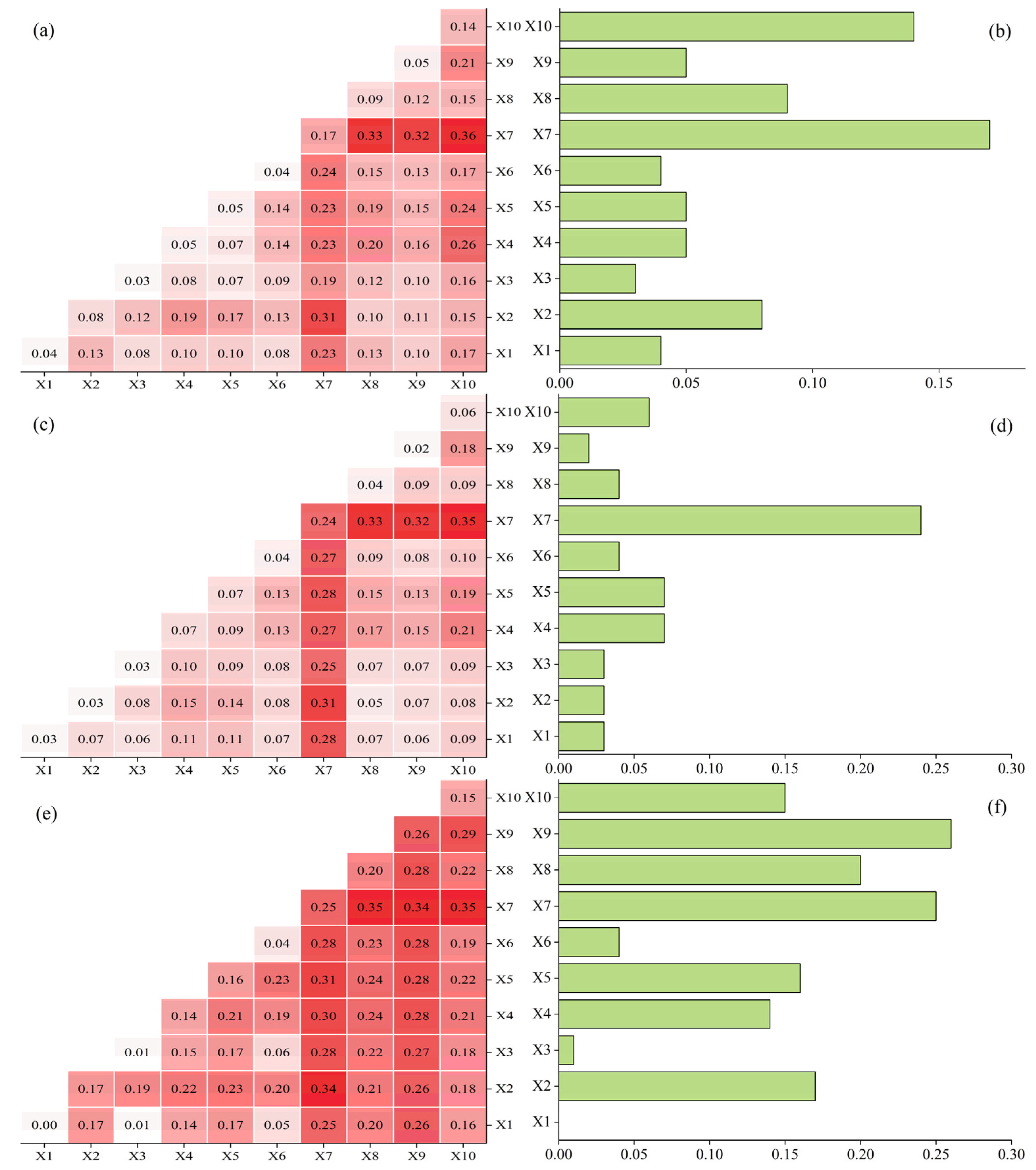
3.3. Factor Detection and Analysis

The results of the factor detection analysis revealed the key driving forces behind vegetation phenology changes and quantified the explanatory power (q-values) of each variable. Specifically, for the start of the growing season (SOS), the dominant driving factors ranked by explanatory power were: X7 > X10 > X8 > X2 > X9 = X5 = X4 > X6 = X1 > X3, with annual precipitation (X7) being the most influential factor (Figure 7b). For the length of the growing season (LOS), the q-value ranking was: X7 > X5 = X4 > X10 > X6 = X8 > X1 = X2 = X3 > X9, again identifying annual precipitation as the dominant factor (Figure 7d). In contrast, the end of the growing season (EOS) was primarily driven by minimum air temperature (X9), followed by annual precipitation and mean temperature, with the q-value ranking as: X9 > X7 > X8 > X2 > X5 > X10 > X4 > X6 > X3 > X1 (Figure 7f). The rise in minimum temperature is likely to accelerate plant senescence due to cumulative cold stress and increased frost frequency. Particularly in autumn and winter, persistently low nighttime temperatures suppress plant metabolic activity and accelerate the degradation of photosynthetic organs—effects that become especially pronounced at the end of the growing season.
To further investigate how interactions between factors affect vegetation phenology, we employed the interaction detector within the OPGD framework to quantify bivariate interaction effects. The results showed that the combined effect of two interacting variables significantly increased the explanatory power for all three phenological indicators (SOS, LOS, and EOS). This increase followed patterns of either bivariate enhancement or nonlinear enhancement, implying that multiple climatic factors act synergistically, exerting far greater influence than individual variables alone. Among the interaction pairs, the combination of annual precipitation and annual maximum temperature exhibited the highest explanatory power on phenological shifts. This interaction strongly influenced seasonal patterns of vegetation growth, particularly under the backdrop of intensifying climate change (Figure 7a,c,e). The coupling of these two climatic variables has profound implications for the spatiotemporal dynamics of plant phenology. These findings highlight the pivotal role of climate interactions—especially between precipitation and maximum temperature—in shaping phenological responses and provide a robust foundation for predicting grassland ecosystem responses to ongoing climate change.

3.4. Analysis of the Influence Mechanism of Grassland Phenology on the South Slope of Qilian Mountains

In this study, we constructed a coupled model integrating multiple phenological indicators of grassland vegetation on the southern slope of the Qilian Mountains using the PLS-SEM (Partial Least Squares Structural Equation Modeling) approach. The aim was to investigate the mechanisms through which climate, topography, and GHG drive changes in vegetation phenology. Model results revealed that the direct path coefficients of climate, topography, and GHG were 0.61, −0.02, and −0.13, respectively (Figure 8). Climate emerged as the dominant driver with the strongest direct influence on vegetation phenology. While topography showed a weak direct effect, it exerted a much stronger indirect influence by regulating climatic conditions and GHG concentrations, with an indirect effect coefficient of 0.49 and a total effect coefficient of 0.47. This highlights topography’s crucial intermediary role in shaping phenological dynamics. GHG had a relatively weak direct impact (−0.13), but their indirect influence through climate mediation was structurally relevant, with an indirect effect coefficient of 0.15 and a total effect of 0.02.
Further analysis revealed that different phenological phases are governed by distinct environmental drivers (Figure 9). Annual precipitation was strongly associated with SOS and LOS, underscoring its importance in determining the timing and duration of grassland growth. In contrast, EOS was primarily affected by annual minimum temperature, suggesting that prolonged low-temperature stress may accelerate plant senescence and reduce late-season physiological activity. Interestingly, SOS was notably correlated with CO2 concentration, indicating that early-season growth may be modulated by carbon assimilation capacity, especially under suboptimal thermal conditions. Meanwhile, LOS and EOS showed stronger correlations with N2O concentrations, highlighting the regulatory role of N2O in the later stages of vegetation development.
As shown in Figure 8, topographic variables affect vegetation phenology indirectly by shaping the spatial distribution of key GHG and climatic factors such as precipitation and minimum temperature. In mountainous environments, terrain plays a foundational role in forming localized climatic regimes and microenvironmental heterogeneity. By influencing the spatial variability of CO2 and N2O concentrations, topography exerts indirect yet pivotal control over phenological processes via climate-mediated pathways. These findings provide valuable insights into ecosystem monitoring, ecological forecasting, and landscape-level management in topographically complex and climate-sensitive regions.
The shape of the ellipse reflects the absolute value of the correlation coefficient: the more elongated the ellipse, the stronger the correlation; the closer it is to a circle, the weaker the correlation. The orientation of the ellipse indicates the direction of the correlation: an upward tilt to the right represents a positive correlation, while a downward tilt to the right represents a negative correlation. The color gradient represents the magnitude and direction of the correlation coefficient, with blue indicating a positive correlation and red indicating a negative correlation.

4. Discussion

This study disentangles the direct and indirect effects of topography, meteorological variables, and GHG on grassland phenology on the southern slope of the Qilian Mountains through a multi-factor coupling framework. The results show that temperature and precipitation exert significant direct effects on the variation in SOS, EOS, and LOS. These findings are consistent with those from other semi-arid and alpine regions such as the Tibetan Plateau and the northern China, reaffirming the dominant role of climate variability in shaping phenological responses [70,71]. Meanwhile, the effects of CO2, CH4, and N2O on phenology are primarily indirect, aligning with prior studies that attribute such influences to altered plant photosynthetic efficiency and nutrient uptake [72,73].
Although topographic variables such as elevation and slope directly impact phenological metrics is weak, they significantly modulate local climate and the spatial distribution of GHG concentrations. This “topography–GHG–phenology” interaction mechanism, which has received limited attention in previous research, provides novel insights into how complex terrain indirectly influences phenological patterns via microclimatic and GHG distribution effects.
PLS-SEM was selected for its ability to address multicollinearity among variables and identify mediation pathways in complex ecological systems. However, this method assumes a predefined linear causal structure, which may limit its capacity to capture nonlinear feedback that are common in real-world ecosystems [74]. Future studies could incorporate Bayesian SEM or nonlinear structural models to enhance flexibility and improve the robustness of causal inference.
The regional differences in GHG within the study area and the spatial scales at which they were harmonized prior to the combined analysis are reasonable for exploring the combined effects of multiple factors. Nonetheless, studies employing finer spatial resolution GHG data would better capture environmental heterogeneity characteristic of mountainous regions. The integration of high-resolution satellite retrievals (e.g., TROPOMI) and in situ observations is recommended to improve spatial characterization of GHGs in future research [75]. The exclusion of variables such as soil moisture, solar radiation, wind speed, and extreme weather events was due to the trade-offs between data availability, spatiotemporal coverage, and model complexity. For example, soil moisture closely regulates the balance between precipitation and evapotranspiration, and its omission may bias the interpretation of precipitation impacts in arid regions [76].
While this study focuses on the southern slope of the Qilian Mountains, the mechanisms revealed—particularly the “meteorological–GHG–phenology” pathway—are likely applicable to other alpine and semi-arid ecosystems, as analogous patterns have been documented in regions such as the Tibetan Plateau [71]. Phenological shifts also have significant implications for global ecosystem functioning. Changes in the timing and length of the growing season can alter carbon uptake, water regulation, and forage availability, indirectly affecting pastoral systems and rural livelihoods [77]. More importantly, phenological asynchrony may disrupt plant–pollinator interactions, leading to reduced reproductive success and heightened risks to biodiversity [78]. Additionally, an earlier EOS or shortened LOS may increase the risk of soil exposure, thereby elevating the risk of erosion and nutrient loss, particularly in steep or fragmented terrains.

5. Conclusions

The SOS of grassland on the southern slope of the Qilian Mountains from 2002 to 2022 was mainly concentrated between 90 and 150 days, LOS was between 120 and 180 days, and EOS was between 240 and 300 days. Spatially, from southeast to northwest, SOS exhibited a gradual delay, LOS showed a progressive shortening, and EOS advanced. Temporally, SOS generally displayed a fluctuating downward trend, with an annual advance of approximately 0.35 days; LOS showed a fluctuating upward trend, lengthening by about 0.55 days per year; and EOS exhibited a fluctuating upward trend, postponing by about 0.20 days annually.
Annual precipitation was identified as the dominant factor influencing both SOS and LOS, while annual minimum temperature played a key role in determining EOS. The combined effect of the two factors had a much greater impact on climate change than either individual factor, showing a bivariate or nonlinear enhancement, with the interaction between annual precipitation and annual maximum temperature having the most significant explanatory power for phenological changes.
Climate factors, particularly annual precipitation, exert a stronger influence on grassland phenology. Topography and GHG regulate the spatial and temporal variability of grassland phenology mainly through their effects on annual precipitation and annual minimum temperature. In addition, topography further affects vegetation phenology indirectly by influencing N2O and CO2.

Author Contributions

Conceptualization, G.C., Q.Z. and L.H.; Data curation, Y.Z.; Funding acquisition, G.C.; Investigation, L.H.; Methodology, M.Z. and Q.Z.; Software, Y.Z., M.Z. and Q.Z.; Supervision, L.H.; Visualization, Q.Z.; Writing—original draft, Y.Z.; Writing—review and editing, Y.Z., G.C., M.Z. and L.H. All authors have read and agreed to the published version of the manuscript.

Funding

This research was funded by the Natural Science Foundation of the Qinghai Province (grant no. 2023-ZJ-907M).

Institutional Review Board Statement

Not applicable.

Informed Consent Statement

Not applicable.

Data Availability Statement

The original contributions presented in this study are included in the article. Further inquiries can be directed to the corresponding author.

Conflicts of Interest

The authors declare no conflicts of interest.

References

  1. Duveiller, G.; Hooker, J.; Cescatti, A. The mark of vegetation change on Earth’s surface energy balance. Nat. Commun. 2018, 9, 679. [Google Scholar] [CrossRef] [PubMed]
  2. Piao, S.; Wang, X.; Park, T.; Chen, C.; Lian, X.; He, Y.; Bjerke, J.W.; Chen, A.; Ciais, P.; Tømmervik, H.; et al. Characteristics, drivers and feedbacks of global greening. Nat. Rev. Earth Environ. 2020, 1, 14–27. [Google Scholar] [CrossRef]
  3. Zhu, K.Z.; Wan, M.W. Phenology; Science Press: Beijing, China, 1973; pp. 2–6. [Google Scholar]
  4. Madiniyati, D.; Yusupujiang, R.; Jiang, H. Temporal and spatial variation of vegetation phenology and its driving factor analysis in the Bosten Lake Drainage Basin from 2001 to 2014. Acta Ecol. Sin. 2018, 38, 6921–6931. [Google Scholar]
  5. Roetzer, T.; Wittenzeller, M.; Haeckel, H.; Nekovar, J. Phenology in central europe–differences and trends of spring phenophases in urban and rural areas. Int. J. Biometeorol. 2000, 44, 60–66. [Google Scholar] [CrossRef]
  6. Du, Q.; Liu, H.; Li, Y.; Xu, L.; Diloksumpun, S. The effect of phenology on the carbon exchange process in grassland and maize cropland ecosystems across a semiarid area of China. Sci. Total Environ. 2019, 695, 133868. [Google Scholar] [CrossRef]
  7. Zhang, Z.; Zhou, J.; Yuan, Y.; Wang, X.; Chen, B.; Zhang, H.; Xin, X. Estimating the impact of climate change on the carbon exchange of a temperate meadow steppe in China. Ecol. Indic. 2022, 140, 109055. [Google Scholar] [CrossRef]
  8. Shen, P.; Wang, X.; Zohner, C.M.; Peñelas, J.; Zhou, Y.; Tang, Z.; Xia, J.; Zheng, H.; Fu, Y.; Liang, J.; et al. Biodiversity buffers the response of spring leaf unfolding to climate warming. Nat. Clim. Change 2024, 14, 863–868. [Google Scholar] [CrossRef]
  9. Dong, S. Revitalizing the grassland on the Qinghai–Tibetan Plateau. Grassl. Res. 2023, 2, 241–250. [Google Scholar] [CrossRef]
  10. Huang, Z.; Liu, Y.; Cui, Z.; Liu, Y.; Wang, D.; Tian, F.; Wu, G. Natural grasslands maintain soil water sustainability better than planted grasslands in arid areas. Agric. Ecosyst. Environ. 2019, 286, 106683. [Google Scholar] [CrossRef]
  11. Masson-Delmotte, V.; Zhai, P.; Pirani, A.; Connors, S.L.; Péan, C.; Berger, S.; Caud, N.; Chen, Y.; Goldfarb, L.; Gomis, M.I.; et al. IPCC, 2021: Climate Change 2021: The Physical Science Basis. Contribution of Working Group I to the Sixth Assessment Report of the Intergovernmental Panel on Climate Change; Cambridge University Press: Cambridge, UK, 2021. [Google Scholar]
  12. Li, H.; Ma, Y.; Wang, Y. Influences of climate warming on plant phenology in Qinghai plateau. J. Appl. Meteorol. Sci. 2010, 21, 500–505. [Google Scholar]
  13. Currier, C.M.; Sala, O.E. Precipitation versus temperature as phenology controls in drylands. Ecology 2022, 103, e3793. [Google Scholar] [CrossRef] [PubMed]
  14. Sun, M.; Li, P.; Ren, P.; Tang, J.; Zhang, C.; Zhou, X.; Peng, C. Divergent response of vegetation phenology to extreme temperatures and precipitation of different intensities on the Tibetan Plateau. Sci. China Earth Sci. 2023, 66, 2200–2221. [Google Scholar] [CrossRef]
  15. Li, C.; Zou, Y.; He, J.; Zhang, W.; Gao, L.; Zhuang, D. Response of Vegetation Phenology to the Interaction of Temperature and Precipitation Changes in Qilian Mountains. Remote Sens. 2022, 14, 1248. [Google Scholar] [CrossRef]
  16. Wang, Y.; Liu, Y.; Zhou, L.; Zhou, G. Spatiotemporal patterns of phenological metrics and their relationships with environmental drivers in grasslands. Sci. Total Environ. 2024, 938, 173489. [Google Scholar] [CrossRef]
  17. Skakun, S.; Franch, B.; Vermote, E.; Roger, J.C.; Becker-Reshef, I.; Justice, C.; Kussul, N. Early season large-area winter crop mapping using MODIS NDVI data, growing degree days information and a Gaussian mixture model. Remote Sens. Environ. 2017, 195, 244–258. [Google Scholar] [CrossRef]
  18. Su, F.; Wang, J.; Wang, Z.; Chen, Y.; Wang, L.; Yang, K. Temporal and Spatial Changes of Vegetation Phenology and Its Response to Climate Change in Nanpan River Basin from 2001 to 2020. Res. Soil Water Conserv. 2022, 29, 220–227. [Google Scholar]
  19. Tang, Y.; Sun, H.; Wang, X. Using leaf area index to analyze the growth stability and influencing factors of the Mount Altai Taiga under climate change. Acta Ecol. Sin. 2024, 44, 8258–8268. [Google Scholar]
  20. Li, X.; Zeng, F.; Jiang, Q.; Yan, S. Remote sensing monitoring of vegetation phonological features in songnen plain of northeast China during 1999–2013. J. Nat. Resour. 2017, 32, 321–328. [Google Scholar]
  21. Zhang, Y.; Hong, S.; Liu, Q.; Huntingord, C.; Peñuelas, J.; Rossi, S. Autumn canopy senescence has slowed down with global warming since the 1980s in the Northern Hemisphere. Commun. Earth Environ. 2023, 4, 173. [Google Scholar] [CrossRef]
  22. Liu, N.; Ding, Y.; Peng, S. Temporal effects of climate on vegetation trigger the response biases of vegetation to human activities. Glob. Ecol. Conserv. 2021, 31, e01822. [Google Scholar] [CrossRef]
  23. Cui, H.; Chu, L.; Yin, Y.; Pan, Y.; Meng, H.; Wang, T. Spatio-temporal patterns of vegetation phenology and their evolutionary mechanisms in the Three Gorges Reservoir Area from 1990 to 2020. Acta Ecol. Sin. 2024, 44, 3775–3790. [Google Scholar]
  24. Ontel, I.; Avram, S.; Gheorghe, C.A.; Niculae, M.I.; Pascu, I.S.; Rodino, S. Shifting vegetation phenology in protected areas: A response to climate change. Ecol. Inform. 2025, 85, 102962. [Google Scholar] [CrossRef]
  25. Liu, Q.; Fu, Y.H.; Zhu, Z.; Liu, Y.; Liu, Z.; Huang, M.; Janssens, I.A.; Piao, S. Delayed autumn phenology in the Northern Hemisphere is related to change in both climate and spring phenology. Glob. Change Biol. 2016, 22, 3702–3711. [Google Scholar] [CrossRef]
  26. Linkosalmi, M.; Tuovinen, J.-P.; Nevalainen, O.; Peltoniemi, M.; Taniş, C.M.; Arslan, A.N.; Rainne, J.; Lohila, A.; Laurila, T.; Aurela, M. Tracking Vegetation Phenology of Pristine Northern Boreal Peatlands by Combining Digital Photography with CO2 Flux and Remote Sensing Data. Biogeosciences 2022, 19, 4747–4765. [Google Scholar] [CrossRef]
  27. Zhou, G.; Song, X.; Zhou, M.; Zhou, L.; Ji, Y. Advances in influencing mechanism and model of total climatic production factors of plant phenology change. Sci. Sin. 2023, 3, 380–389. [Google Scholar] [CrossRef]
  28. Delpierre, N.; Vitasse, Y.; Chuine, I.; Guillemot, J.; Bazot, S.; Rutishauser, T.; Rathgeber, C.B. Temperate and boreal forest tree phenology: Fromorgan-scale processes to terrestrial ecosystem models. Ann. For. Sci. 2016, 73, 5–25. [Google Scholar] [CrossRef]
  29. Chen, L.; Huang, J.G.; Ma, Q.; Hänninen, H.; Tremblay, F.; Bergeron, Y. Long-term changes in the impacts of global warming on leaf phenology of four temperate tree species. Glob. Change Biol. 2019, 25, 997–1004. [Google Scholar] [CrossRef]
  30. Sun, M.; Zhang, Y.; Xin, Y.; Zhong, D.; Yang, C. Changes of Vegetation Phenology and Its Response to Climate Change in the West Sichuan Plateau in the Past 20 Years. Ecol. Environ. 2022, 31, 1326–1339. [Google Scholar]
  31. Jiang, Z.; Sun, Y.; Zhao, S.; He, W.; Li, Z. Vegetation Phenological Change and Its Response to Climate Change in Qinghai Province. J. Ecol. Rural. Environ. 2022, 38, 765–776. [Google Scholar]
  32. Li, D.; Wang, Z. Spatiotemporal Variation of Vegetation Phenology and Its Response to Climate in Qinling Mountains Based on MCD12Q2. Ecol. Environ. Sci. 2020, 1, 11–22. [Google Scholar]
  33. Liu, J.; Li, C.; Li, T.; Liu, Y. The effects of future climate change on soybean growth period and yield in Henan province under RCP scenario. Hubei Agric. Sci. 2020, 22, 81–85. [Google Scholar]
  34. Kong, D.; Zhang, Q.; Huang, W.; Gu, X. Vegetation phenology change in Tibetan Plateau from 1982 to 2013 and its related meteorological factors. Acta Geogr. Sin. 2017, 1, 39–52. [Google Scholar]
  35. Xiong, X.; Li, C.; Chen, J. Topographic regulatory role of vegetation response to climate change. Acta Geogr. Sin. 2023, 78, 2256–2270. [Google Scholar]
  36. Meng, F.; Hong, S.; Wang, J.; Chen, A.; Zhang, Y.; Zhang, Y.; Janssens, I.A.; Mao, J.; Myneni, R.B.; Peñuelas, J.; et al. Climate change increases carbon allocation to leaves in early leaf green-up. Ecol. Lett. 2023, 26, 816–826. [Google Scholar] [CrossRef]
  37. Menzel, A.; Sparks, T.H.; Estrella, N.; Koch, E.; Aasa, A.; Ahas, R.; Alm-Kübler, K.; Bissolli, P.; Braslavská, O.G.; Briede, A.; et al. European phenological response to climate change matches the warming pattern. Nature 2006, 437, 559–562. [Google Scholar] [CrossRef]
  38. Wang, J.; Xu, C. Geodetector: Principle and prospective. Acta Geogr. Sin. 2017, 72, 116–134. [Google Scholar]
  39. Song, Y.; Wang, J.; Ge, Y.; Xu, C. An optimal parameters-based geographical detector model enhances geographic characteristics of explanatory variables for spatial heterogeneity analysis: Cases with different types of spatial data. GIScience Remote Sens. 2020, 57, 593–610. [Google Scholar] [CrossRef]
  40. She, Y.; Zhang, Y.; Chen, C. Temporal and spatial dynamics of NDVI and its driving force analysis in Hunan Province from 2000 to 2020. J. Cent. South Univ. For. Technol. 2025, 4, 108–118. [Google Scholar]
  41. Luo, K.; Samat, A.; Van de Voorde, T.; Li, W.; Xu, W.; Abuduwaili, J. Assessing Ecological Quality Dynamics and Driving Factors in the Irtysh River Basin Using AWBEI and OPGD Approaches. IEEE J. Sel. Top. Appl. Earth Obs. Remote Sens. 2025, 18, 1153–1173. [Google Scholar] [CrossRef]
  42. Jin, Y.; Wang, F.; Zong, Q.; Jin, K.; Liu, C.; Qin, P. Spatial patterns and driving forces of urban vegetation greenness in China: A case study comprising 289 cities. Geogr. Sustain. 2024, 5, 370–381. [Google Scholar] [CrossRef]
  43. Tenenhaus, M.; Vinzi, W.E.; Chatelin, Y.M.; Lauro, C. PLS path modeling. Comput. Stat. Data Anal. 2005, 48, 159–205. [Google Scholar] [CrossRef]
  44. Liu, Z.; Si, J.; Deng, Y.; Jia, B.; Li, X.; He, X.; Zhou, D.; Wang, C.; Zhu, X.; Qin, J.; et al. Assessment of Land Desertification and Its Drivers in Semi-Arid Alpine Mountains: A Case Study of the Qilian Mountains Region, Northwest China. Remote Sens. 2023, 15, 3836. [Google Scholar] [CrossRef]
  45. Wang, H.; Xiong, X.; Wang, K.; Li, X.; Hu, H.; Li, Q.; Yin, H.; Wu, C. The effects of land use on water quality of alpine rivers: A case study in Qilian Mountain, China. Sci. Total Environ. 2023, 875, 162696. [Google Scholar] [CrossRef]
  46. Jia, Z.; Lin, T.; Guo, X.; Zheng, Y.; Geng, H.; Zhang, J.; Chen, Y.; Liu, W.; Lin, M. Vegetation greening mitigates the positive impacts of climate change on water availability in northwest China. J. Hydrol. 2024, 644, 132086. [Google Scholar] [CrossRef]
  47. Li, J.; Gong, C. Effects of terrain factors on vegetation cover change in national park of Qilian mountains. Bull. Soil Water Conserv. 2021, 41, 228–237. [Google Scholar]
  48. Tong, S.; Cao, G.; Yan, X.; Diao, E.; Zhang, Z. Spatial-Temporal Evolution of Vegetation Cover and its Driving Factors on the South Slope of the Qilian Mountains, China from 2000 to 2020. Mt. Res. 2022, 40, 491–503. [Google Scholar]
  49. Zhang, Q.; Cao, G.; Zhang, L.; Zhao, M. Spatiotemporal changes in vegetation greenness on the southern slopes of the Qilian Mountains and their responses to climate change and human activities. Arid Zone Res. 2024, 41, 2143–2153. [Google Scholar]
  50. Baranova, A.; Chickhoff, U.; Wang, S.; Jin, M. Mountain pastures of Qilian Shan: Plant communities, grazing impact and degradation status (Gansu province, NW China). Hacquetia 2016, 15, 21–35. [Google Scholar] [CrossRef]
  51. Wang, G.; Zhou, G.; Yang, L.; Li, Z. Distribution, species diversity and life-form spectra of plant communities along an altitudinal gradient in the northern slopes of Qilianshan Mountains, Gansu, China. Plant Ecol. 2003, 165, 169–181. [Google Scholar] [CrossRef]
  52. Qiao, C.; Jia, D.; Cheng, C. Vegetation phenology change and response to temperature in the Qilian Mountains from 1982 to 2014. J. Beijing Norm. Univ. 2022, 1, 168–177. [Google Scholar]
  53. Jia, J.; Liu, H.; Lin, Z. Multi-time scale changes of vegetation NPP in six provinces of northwest China and their responses to climate change. Acta Ecol. Sin. 2019, 14, 5058–5069. [Google Scholar]
  54. Ge, Q.; Dai, J.; Cui, H.; Wang, H. Spatiotemporal Variability in Start and End of Growing Season in China Related to Climate Variability. Remote Sens. 2016, 8, 433. [Google Scholar] [CrossRef]
  55. Zhou, Y.; Liu, J. Spatio-temporal Analysis of Vegetation Phenology with Multiple Methods over the Tibetan Plateau based on MODIS NDVI Data. Remote Sens. Technol. Appl. 2018, 3, 486–498. [Google Scholar]
  56. Guan, Q.; Ding, M.; Zhang, H. Spatiotemporal Variation of Spring Phenology in Alpine Grassland and Response to Climate Changes on the Qinghai-Tibet, China. Mt. Res. 2019, 37, 639–648. [Google Scholar]
  57. Ji, Z.; Pei, T.; Chen, Y.; Hou, Q.; Xie, B.; Wu, H. Grassland phenological dynamics and its response to driving factors on the Qinghai-Tibet Plateau. Pratacultural Sci. 2023, 40, 4–14. [Google Scholar]
  58. Zhao, X.; Liu, Y.; Yang, S.; Zhang, Q.; Gao, F.; Liu, Y. Spatio-temporal variations of typical woodland and grassland phenology and its response to meteorological factors in Northern China. Acta Ecol. Sin. 2023, 43, 3744–3755. [Google Scholar]
  59. Savitzky, A.; Golay, M.J.E. Smoothing and differentiation of data by simplified least squares procedures. Anal. Chem. 1964, 36, 1627–1639. [Google Scholar] [CrossRef]
  60. Xie, H.; Li, J.; Tong, X.; Zhang, J.; Liu, P.; Yu, P.; Hu, H.; Yang, M. Spatial-temporal variations of forest and grassland phenology in the Yellow River Basin during 2000-2018. Chin. J. Appl. Ecol. 2023, 34, 647–656. [Google Scholar]
  61. Yuan, M.; Wen, Z.; He, L.; Li, X.; Zhao, L. Response of temperate grassland phenology to climate change and its contribution to gross primary productivity in China. Acta Ecol. Sin. 2024, 44, 354–376. [Google Scholar]
  62. Sen, P. Estimates of the Regression Coefficient Based on Kendall’s Tau. J. Am. Stat. Assoc. 2012, 63, 1379–1389. [Google Scholar] [CrossRef]
  63. Zhang, Q.; Cao, G.; Zhao, M.; Zhang, Y. kNDVI Spatiotemporal Variations and Climate Lag on Qilian Southern Slope: Sen–Mann–Kendall and Hurst Index Analyses for Ecological Insights. Forests 2025, 16, 307. [Google Scholar] [CrossRef]
  64. Frimpong, B.F.; Koranteng, A.; Molkenthin, F. Analysis of temperature variability utilising Mann–Kendall and Sen’s slope estimator tests in the Accra and Kumasi Metropolises in Ghana. Environ. Syst. Res. 2022, 11, 24. [Google Scholar] [CrossRef]
  65. Mann, H.B. Nonparametric Tests Against Trend. Econometrica 1945, 13, 245–259. [Google Scholar] [CrossRef]
  66. Zhang, M.; Kafy, A.-A.; Ren, B.; Zhang, Y.; Tan, S.; Li, J. Application of the Optimal Parameter Geographic Detector Model in the Identification of Influencing Factors of Ecological Quality in Guangzhou, China. Land 2022, 11, 1303. [Google Scholar] [CrossRef]
  67. Yao, X.; Ye, B.; Lan, Y.; Lin, Z.; Zhu, Z.; Yang, F.; Zeng, X. Diurnal contrast of urban park cooling effects in a “Furnace city” using multi-source geospatial data and optimal parameters-based geographical detector model. Sustain. Cities Soc. 2024, 114, 105765. [Google Scholar] [CrossRef]
  68. Wang, C.; Ma, L.; Zhang, Y.; Chen, N.; Wang, W. Spatiotemporal dynamics of wetlands and their driving factors based on PLS-SEM: A case study in Wuhan. Sci. Total Environ. 2022, 806, 151310. [Google Scholar] [CrossRef]
  69. Shi, J.; Zhang, P.; Liu, Y.; Tian, L.; Cao, Y.; Guo, Y.; Li, J.; Wang, Y.; Huang, J.; Jin, R.; et al. Study on spatiotemporal changes of wetlands based on PLS-SEM and PLUS model: The case of the Sanjiang Plain. Ecol. Indic. 2024, 169, 112812. [Google Scholar] [CrossRef]
  70. Li, Z.; Wu, Y.; Wang, R.; Liu, B.; Qian, Z.; Li, C. Assessment of climatic impact on vegetation spring phenology in Northern China. Atmosphere 2023, 14, 117. [Google Scholar] [CrossRef]
  71. He, X.; Liu, A.; Tian, Z.; Wu, L.; Zhou, G. Response of Vegetation Phenology to Climate Change on the Tibetan Plateau Considering Time-Lag and Cumulative Effects. Remote Sens. 2024, 16, 49. [Google Scholar] [CrossRef]
  72. Zelikova, T.J.; Williams, D.G.; Hoenigman, R.; Blumenthal, D.M.; Morgan, J.A.; Pendall, E. Seasonality of soil moisture mediates responses of ecosystem phenology to elevated CO2 and warming in a semi-arid grassland. J. Ecol. 2015, 103, 1119–1130. [Google Scholar] [CrossRef]
  73. Chen, Y.; Han, M.; Yuan, X.; Hou, Y.; Qin, W.; Zhou, H.; Zhao, X.; Klein, J.A.; Zhu, B. Warming has a minor effect on surface soil organic carbon in alpine meadow ecosystems on the Qinghai-Tibetan Plateau. Global Change Biol. 2022, 28, 1618–1629. [Google Scholar] [CrossRef] [PubMed]
  74. Henseler, J.; Ringle, C.M.; Sarstedt, M. A new criterion for assessing discriminant validity in variance-based structural equation modeling. J. Acad. Mark. Sci. 2015, 43, 115–135. [Google Scholar] [CrossRef]
  75. Yu, X.; Millet, D.B.; Henze, D.K.; Turner, A.J.; Delgado, A.L.; Bloom, A.A.; Sheng, J. A high-resolution satellite-based map of global methane emissions reveals missing wetland, fossil fuel, and monsoon sources. Atmos. Chem. Phys. 2023, 23, 3325–3346. [Google Scholar] [CrossRef]
  76. Teuling, A.J.; Seneviratne, S.I.; Stöckli, R.; Reichstein, M.; Moors, E.; Ciais, P.; Luyssaert, S.; van den Hurk, B.; Ammann, C.; Bernhofer, C.; et al. Contrasting response of European forest and grassland energy exchange to heatwaves. Nat. Geosci. 2010, 3, 722–727. [Google Scholar] [CrossRef]
  77. Wang, J.; Zhou, Z.; Zhu, M.; Wan, J.; Wu, X.; Liu, R.; Zheng, J. Study on the response of Net Primary Productivity to vegetation phenology and its influencing factors in karst ecologically fragile regions. Atmosphere 2024, 15, 1464. [Google Scholar] [CrossRef]
  78. Kudo, G.; Ida, T.Y. Early onset of spring increases the phenological mismatch between plants and pollinators. Ecology 2013, 94, 2311–2320. [Google Scholar] [CrossRef]
Figure 1. The location of the study area.
Atmosphere 16 00653 g001
Figure 2. Flow chart.
Atmosphere 16 00653 g002
Figure 3. Inter-annual variation curves of vegetation phenology.
Atmosphere 16 00653 g003
Figure 4. Spatial distribution of multi-year means of vegetation phenology.
Atmosphere 16 00653 g004
Figure 5. Trends and significance of SOS, LOS, and EOS on the southern slopes of the Qilian Mountains.
Atmosphere 16 00653 g005
Figure 6. Inter-annual variability curves of meteorological data.
Atmosphere 16 00653 g006
Figure 7. (a) SOS two-factor interactive detection; (b) SOS single-factor detection; (c) LOS two-factor interactive detection; (d) LOS single-factor detection; (e) EOS two-factor interactive detection; (f) EOS single-factor detection. Explanatory power of driving factors based on OPGD, where X1 is Aspect, X2 is Altitude, X3 is Slope, X4 is CH4, X5 is N2O, X6 is CO2, X7 is annual precipitation, X8 is Mean air temperature, X9 is Minimum air temperature, and X10 is Maximum air temperature.
Atmosphere 16 00653 g007
Figure 8. Impact analysis of grassland phenological drivers based on the PLS-SEM model, with solid and dashed arrows indicating direct and indirect effects, respectively.
Atmosphere 16 00653 g008
Figure 9. Correlation coefficients between climatic factors and drivers based on the Pearson correlation coefficient method.
Atmosphere 16 00653 g009
Table 1. Data sources.
DatasetSymbolSourceSpatial ResolutionTime ResolutionUse Period
AspectX1https://www.gscloud.cn/ (accessed on 15 October 2024)90 m--
AltitudeX290 m--
SlopeX390 m--
CH4X4https://edgar.jrc.ec.europa.eu/ (accessed on 1 November 2024)0.1°Year2002–2022
N2OX50.1°Year2002–2022
CO2X60.1°Year2002–2022
Annual precipitationX7http://data.cma.cn/ (accessed on 15 October 2024)0.0083333°Year2002–2022
Mean air temperatureX80.0083333°Year2002–2022
Minimum air temperatureX90.0083333°Year2002–2022
Maximum air temperatureX100.0083333°Year2002–2022
Land cover dataset http://www.ncdc.ac.cn (accessed on 15 October 2024)30 mYear2002, 2012, 2022
MOD13A2.061 NDVI https://earthengine.google.com/ (accessed on 20 October 2024)1 km16 Days2001–2023
Disclaimer/Publisher’s Note: The statements, opinions and data contained in all publications are solely those of the individual author(s) and contributor(s) and not of MDPI and/or the editor(s). MDPI and/or the editor(s) disclaim responsibility for any injury to people or property resulting from any ideas, methods, instructions or products referred to in the content.

