Drivers of a Summertime Combined High Air Pollution Event of Ozone and PM2.5 in Taiyuan, China


Abstract
1. Introduction
2. Methodology
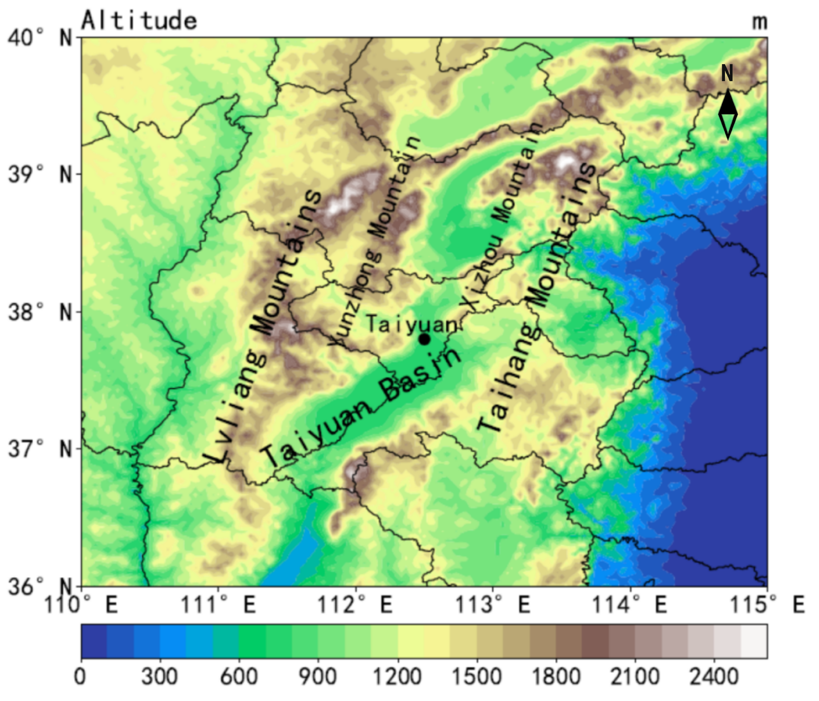
2.1. Measurements
2.2. Model Description
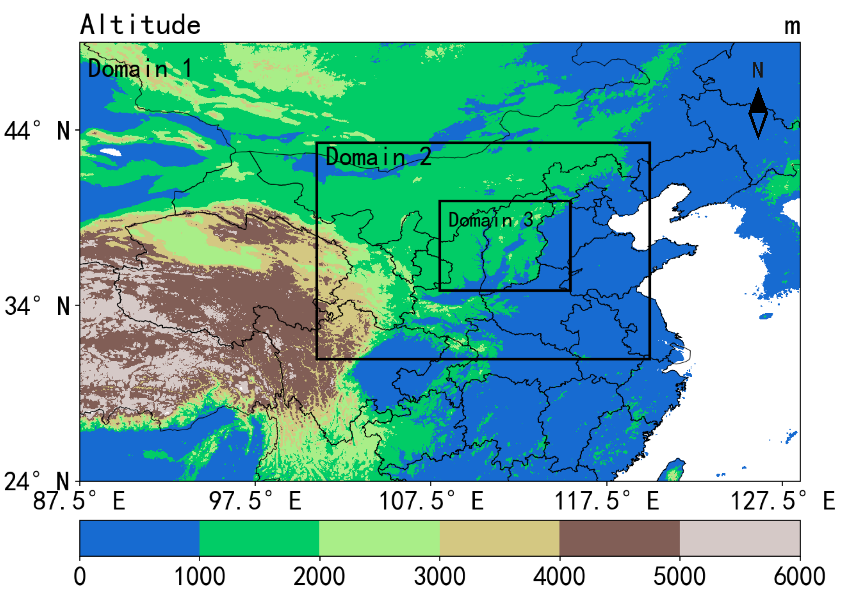
2.2.1. Model Settings
2.2.2. Gas-Phase Chemical Mechanism
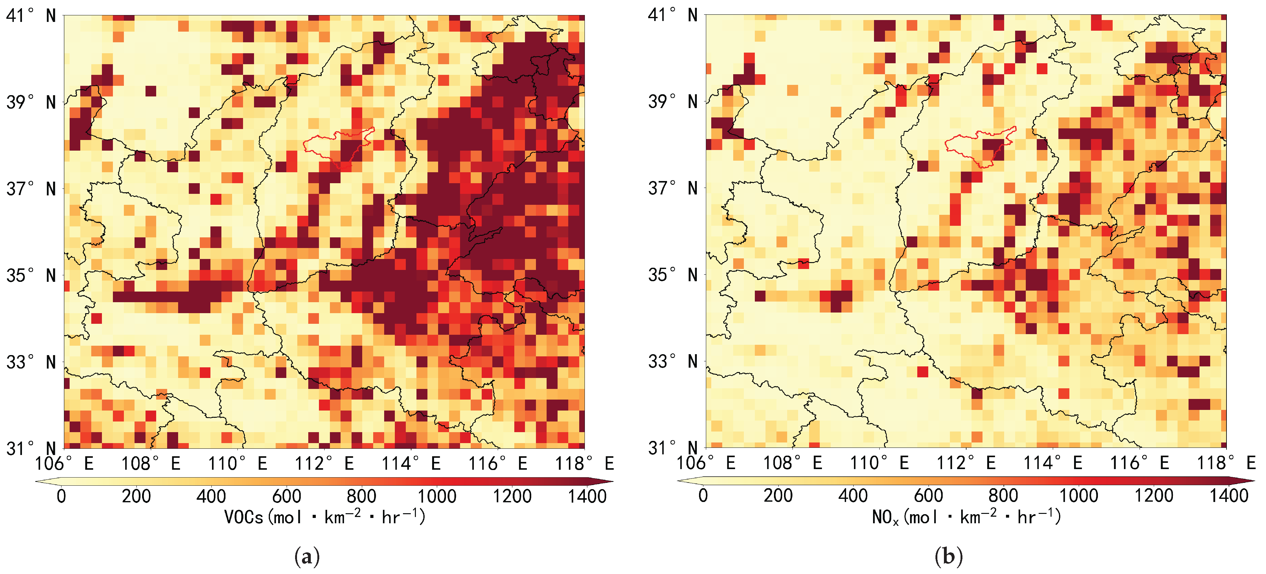
2.2.3. Emissions
2.3. Assessment Parameters
2.4. Sensitivity Tests
3. Results and Discussions
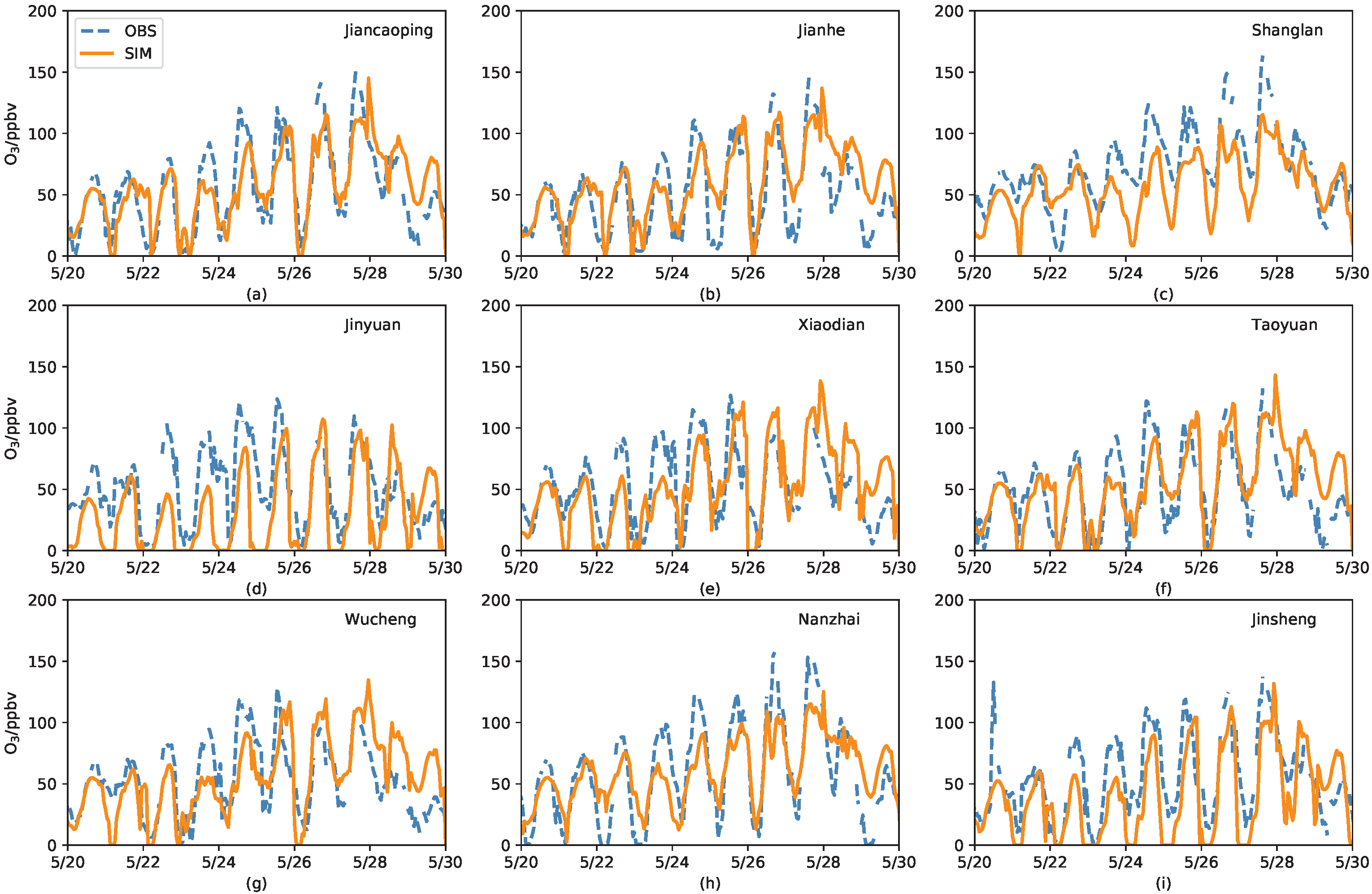
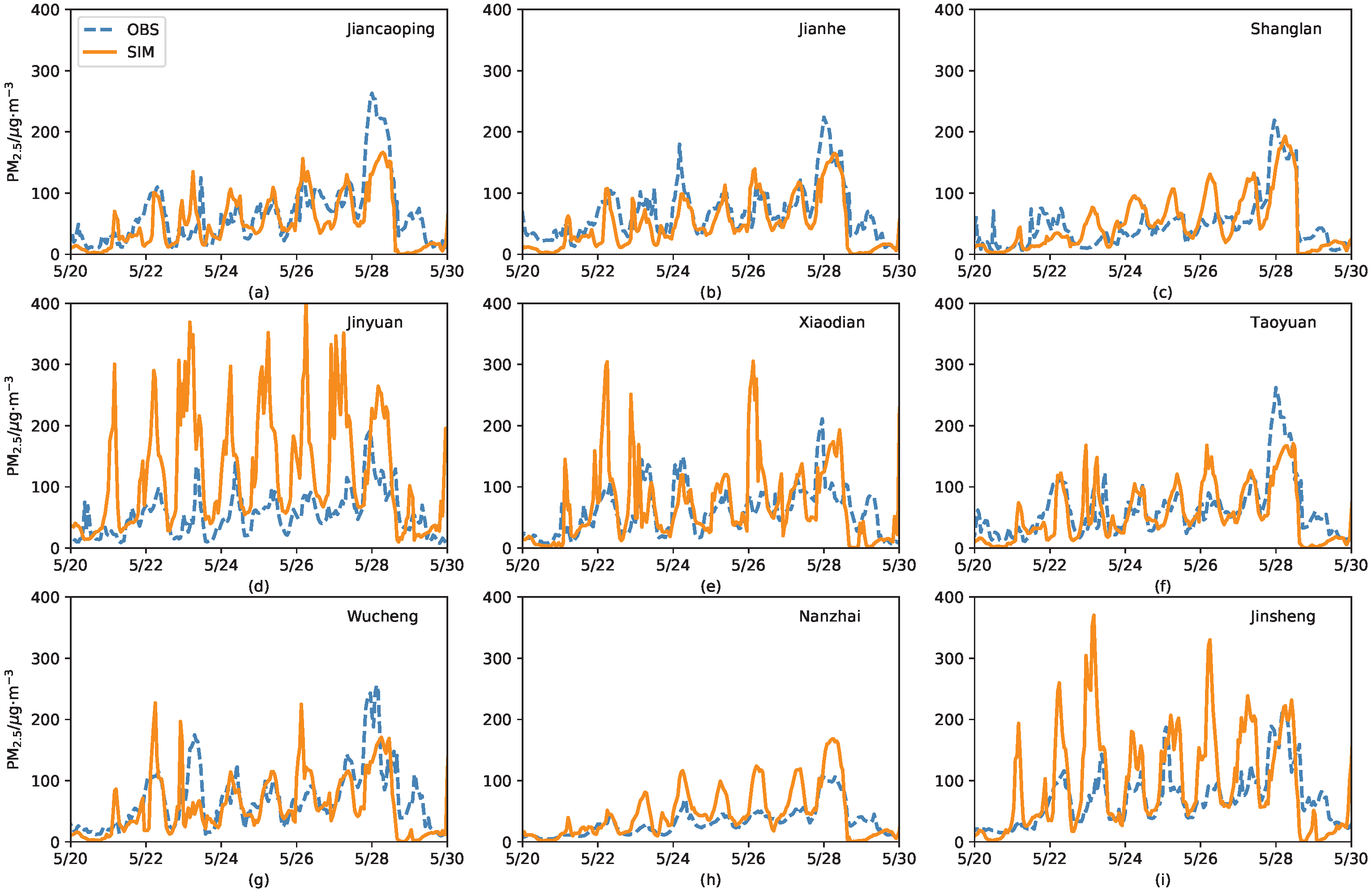
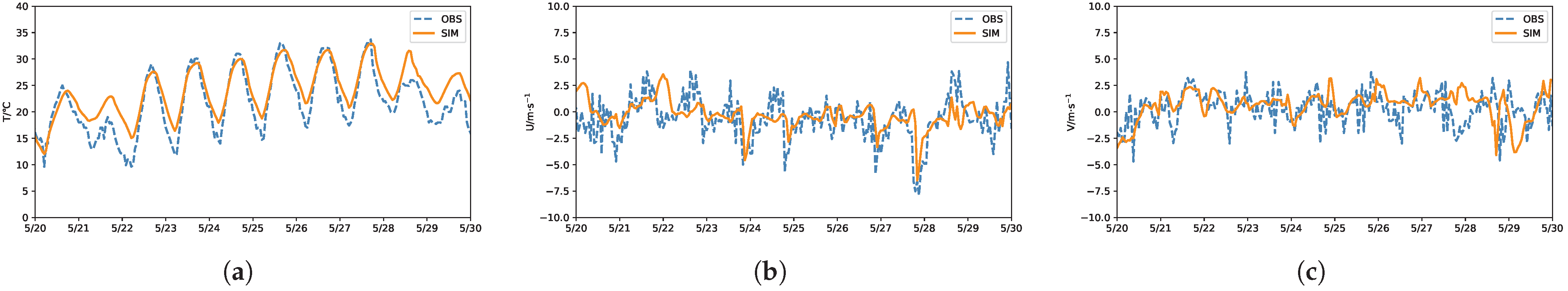
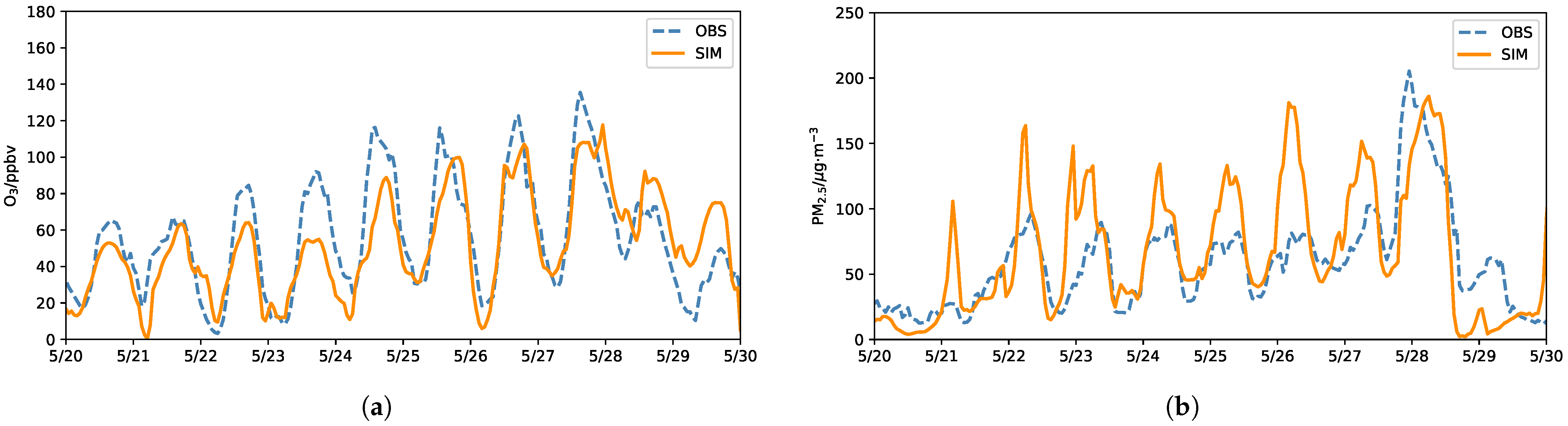
3.1. Comparison of Time Series Between Simulations and Measurements
3.2. Analysis of the Drivers of the Combined Pollution Event in Taiyuan
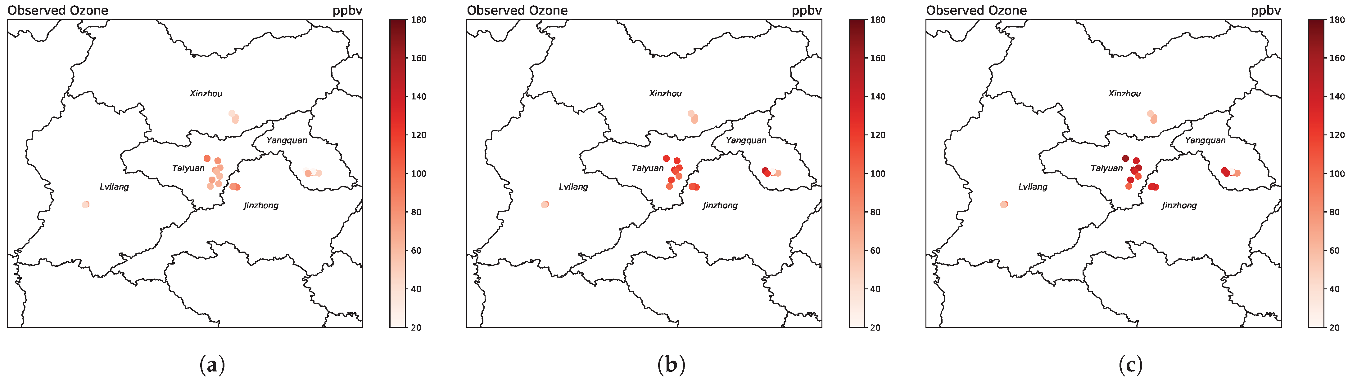
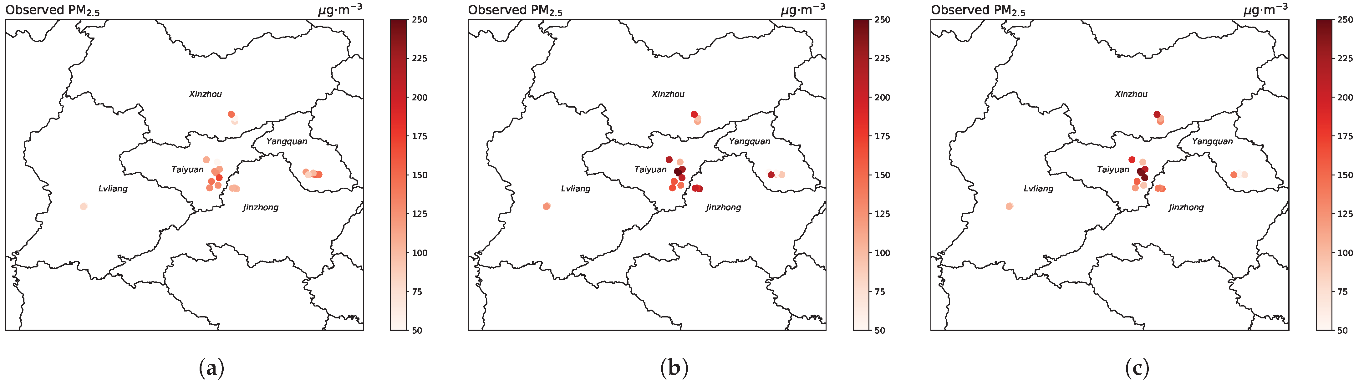
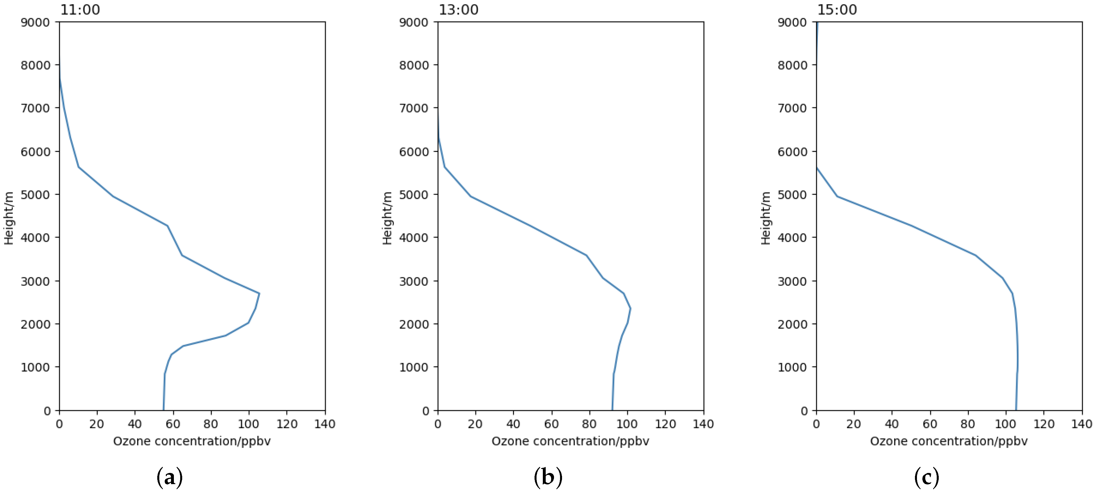
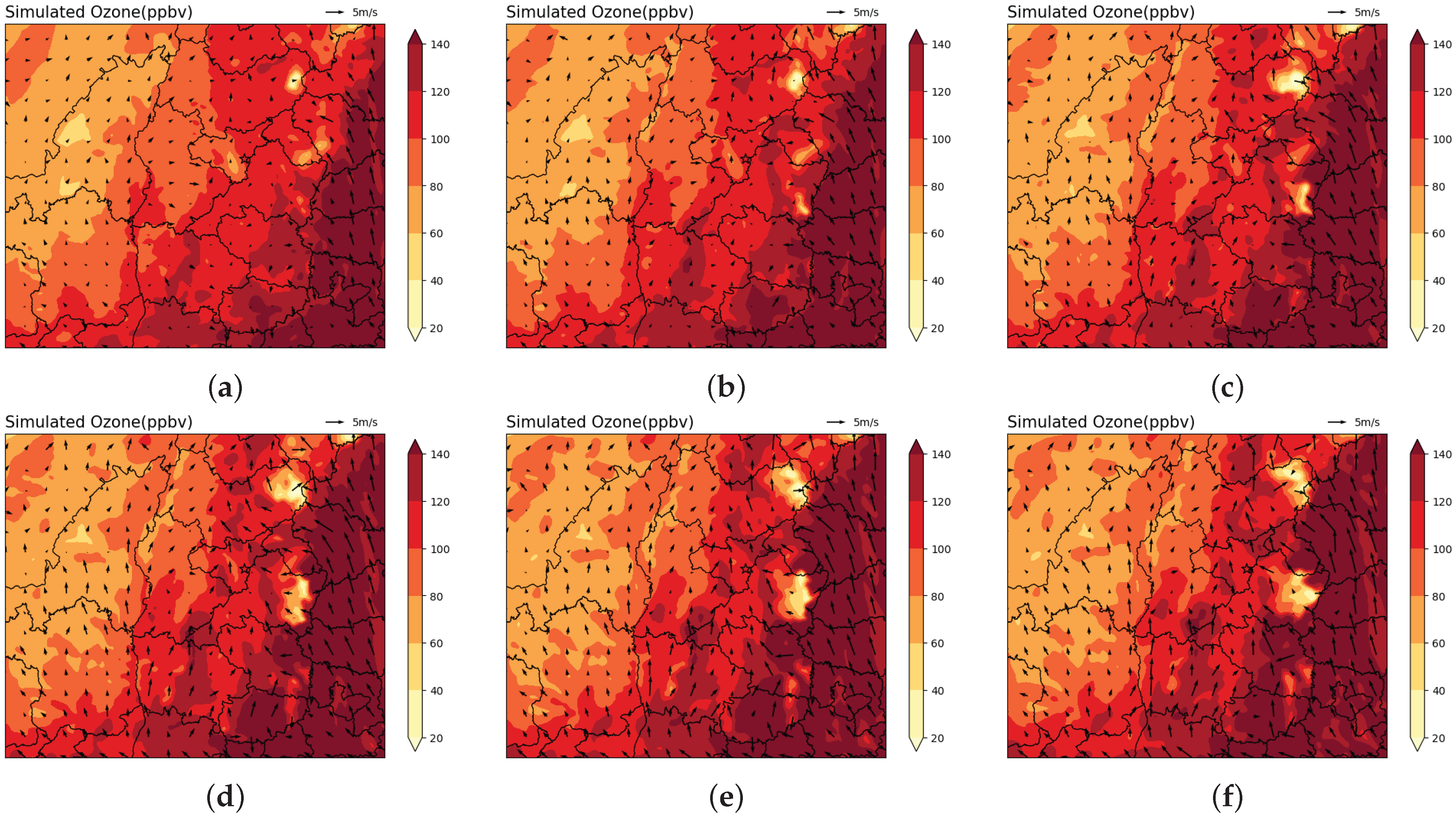
3.2.1. Spatial Distributions of the Observed Ozone and PM2.5
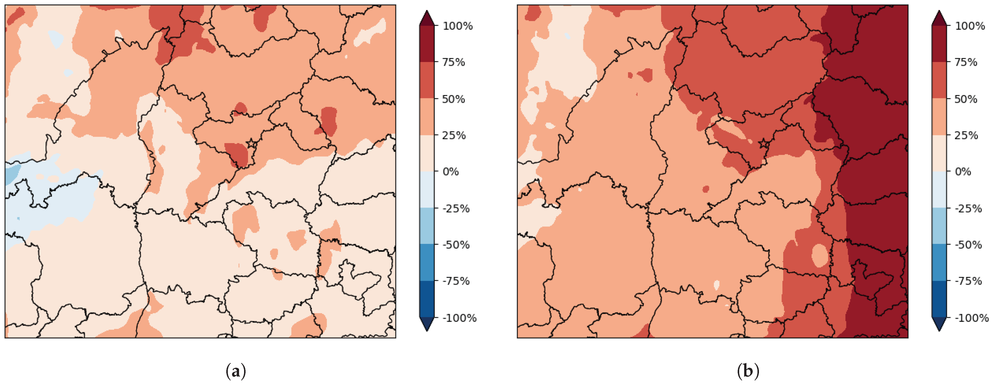
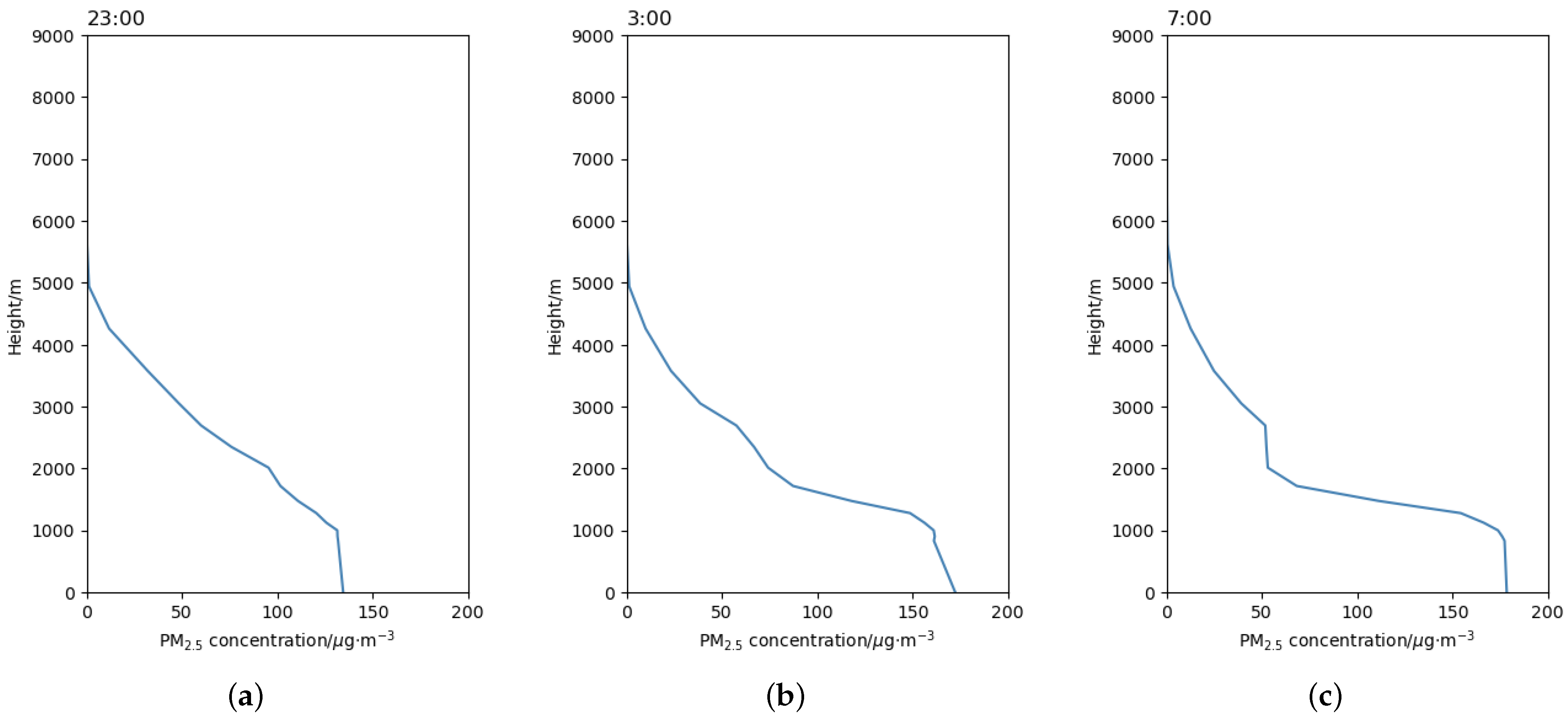
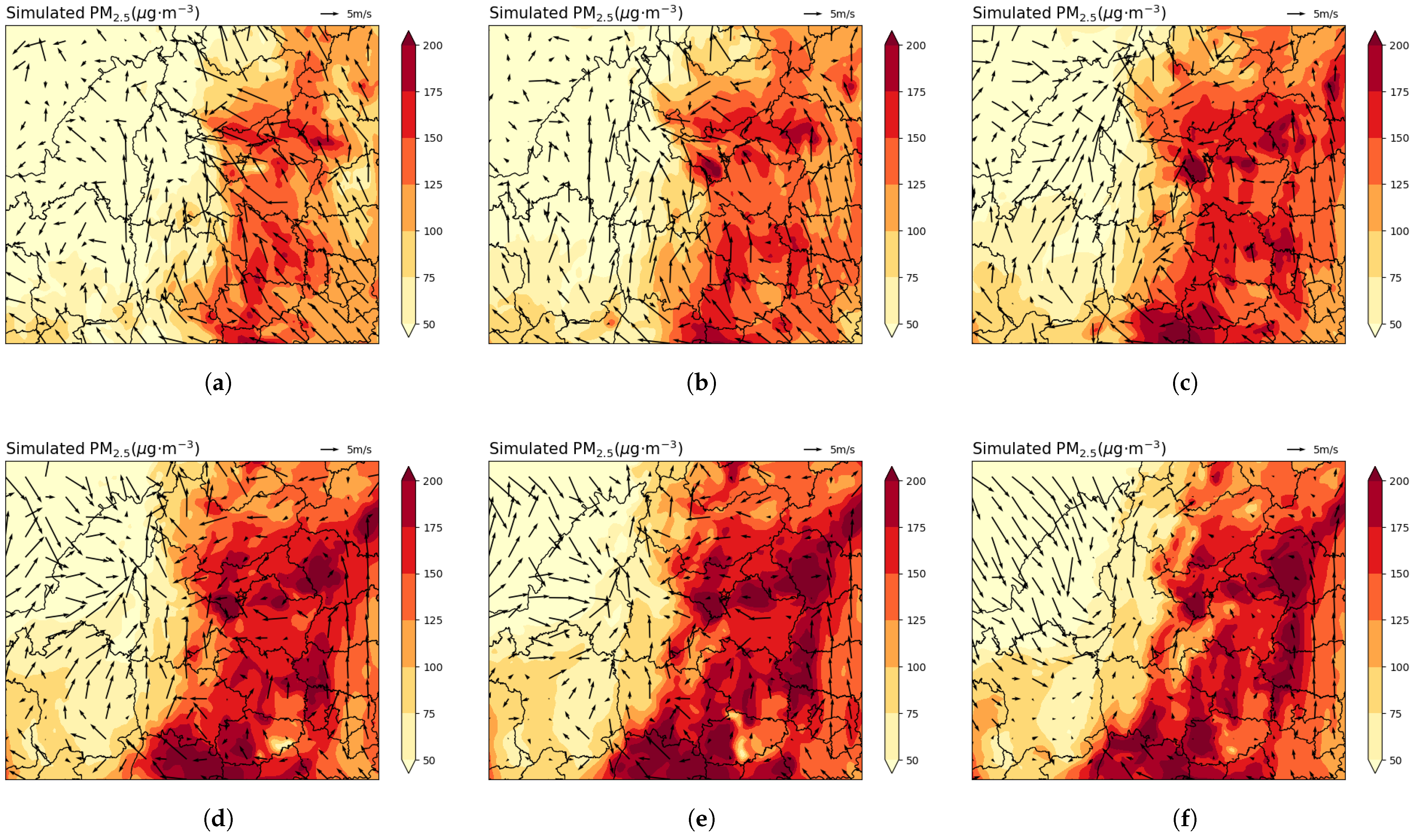
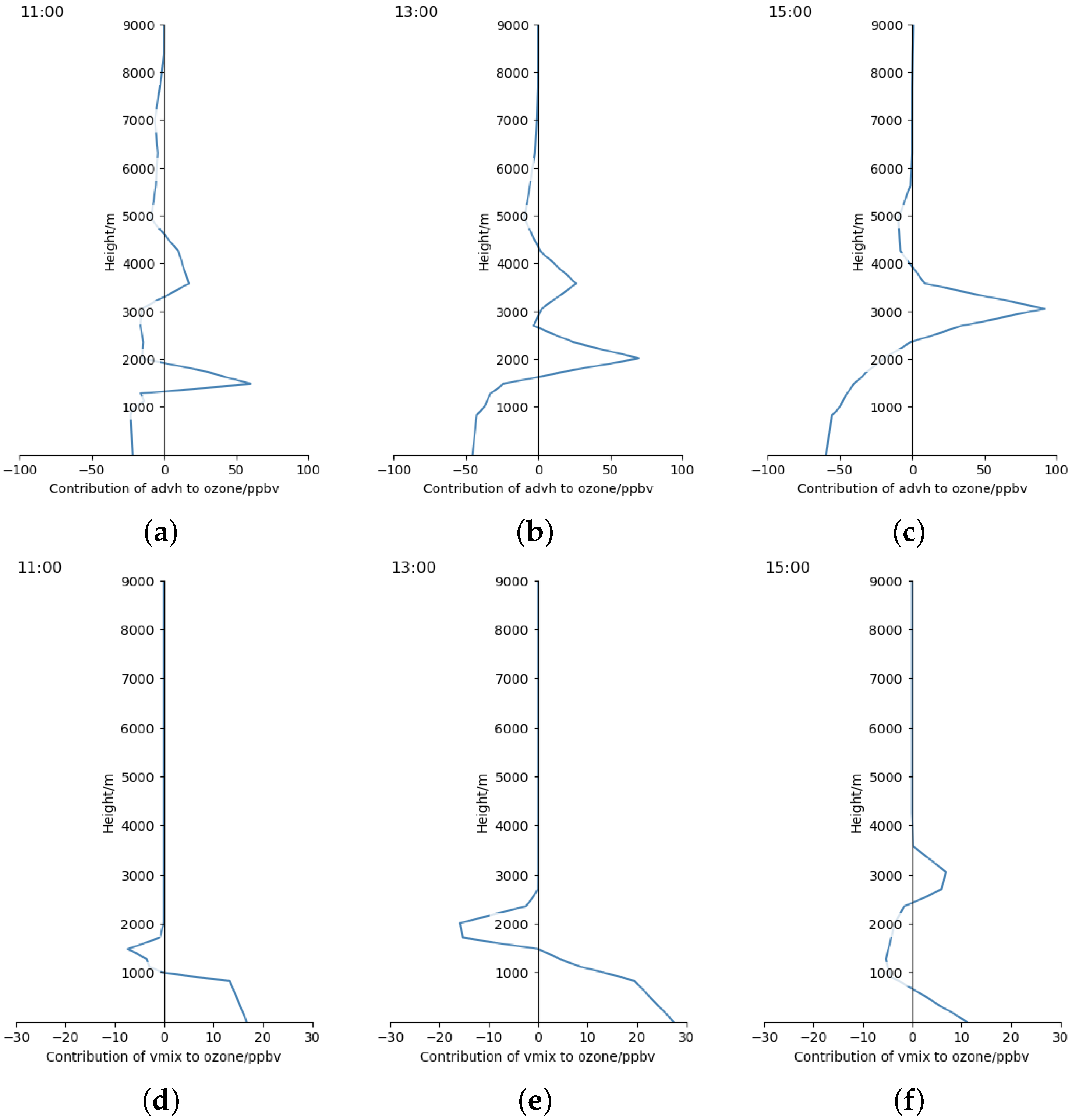
3.2.2. Contributions of the Transport and Emissions to Air Pollution in Taiyuan
4. Conclusions and Future Work
Author Contributions
Funding
Institutional Review Board Statement
Informed Consent Statement
Data Availability Statement
Acknowledgments
Conflicts of Interest
Appendix A. Comparison of Simulated and Observed Concentrations of Ozone and PM 2.5 at Each Monitoring Station
Appendix B. Spatial Distributions of Anthropogenic Emissions of Ozone and PM 2.5 Precursors
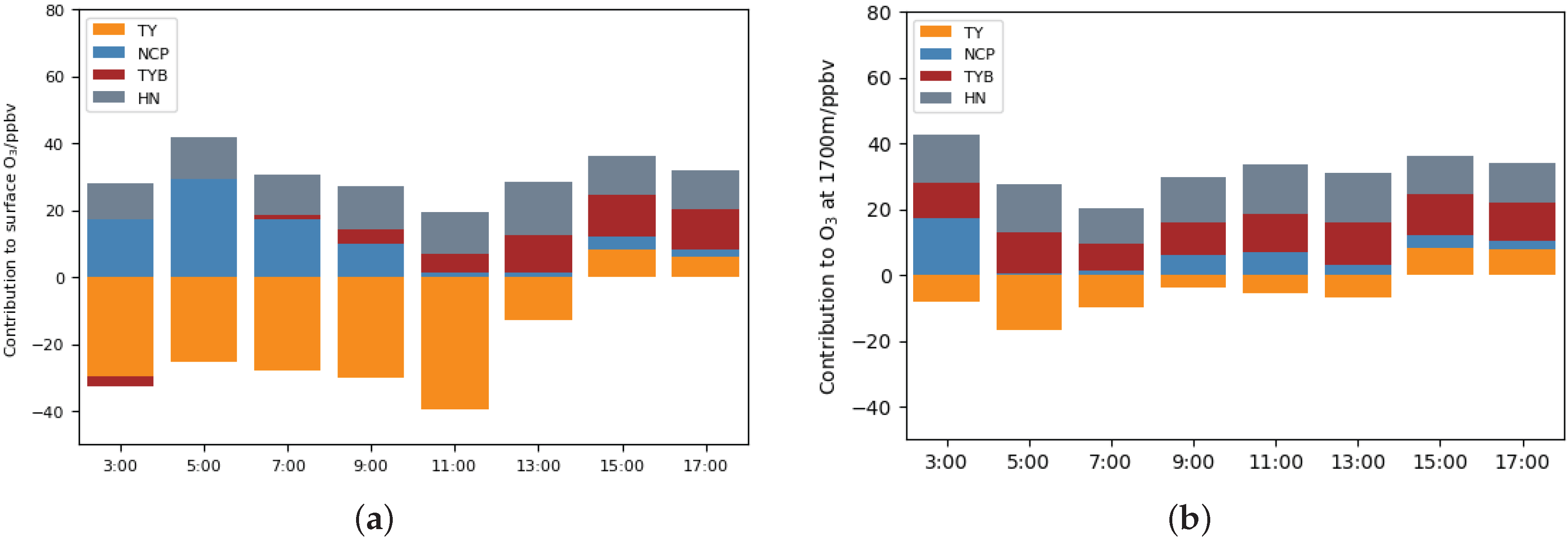
Appendix C. Contributions of Emissions from Different Source Regions to the Air Pollution in Taiyuan

References
- Zong, L.; Yang, Y.; Gao, M.; Wang, H.; Gao, Z. Large-scale synoptic drivers of co-occurring summertime ozone and PM2.5 pollution in eastern China. Atmos. Chem. Phys. 2021, 21, 9105–9124. [Google Scholar] [CrossRef]
- Liu, K.; Shang, Q.; Wan, C. Sources and health risks of heavy metals in PM2.5 in a campus in a typical suburb area of Taiyuan, North China. Atmosphere 2018, 9, 46. [Google Scholar] [CrossRef]
- Chen, Q.; Fu, T.M.; Hu, J.; Ying, Q.; Zhang, L. Modelling secondary organic aerosols in China. Natl. Sci. Rev. 2017, 4, 806–809. [Google Scholar] [CrossRef]
- Li, J.; Cao, L.; Gao, W.; He, L.; Yan, Y.; He, Y.; Pan, Y.; Ji, D.; Liu, Z.; Wang, Y. Seasonal variations in the highly time-resolved aerosol composition, sources and chemical processes of background submicron particles in the North China Plain. Atmos. Chem. Phys. 2021, 21, 4521–4539. [Google Scholar] [CrossRef]
- Jimenez, J.L.; Canagaratna, M.; Donahue, N.; Prevot, A.; Zhang, Q.; Kroll, J.H.; DeCarlo, P.F.; Allan, J.D.; Coe, H.; Ng, N.; et al. Evolution of organic aerosols in the atmosphere. Science 2009, 326, 1525–1529. [Google Scholar] [CrossRef] [PubMed]
- Zhang, Q.; Jimenez, J.L.; Canagaratna, M.R.; Ulbrich, I.M.; Ng, N.L.; Worsnop, D.R.; Sun, Y. Understanding atmospheric organic aerosols via factor analysis of aerosol mass spectrometry: A review. Anal. Bioanal. Chem. 2011, 401, 3045–3067. [Google Scholar] [CrossRef] [PubMed]
- Deng, Y.; Inomata, S.; Sato, K.; Ramasamy, S.; Morino, Y.; Enami, S.; Tanimoto, H. Temperature and acidity dependence of secondary organic aerosol formation from α-pinene ozonolysis with a compact chamber system. Atmos. Chem. Phys. 2021, 21, 5983–6003. [Google Scholar] [CrossRef]
- Shiraiwa, M.; Pöschl, U. Mass accommodation and gas–particle partitioning in secondary organic aerosols: Dependence on diffusivity, volatility, particle-phase reactions, and penetration depth. Atmos. Chem. Phys. 2021, 21, 1565–1580. [Google Scholar] [CrossRef]
- Fu, Y.; Liao, H.; Yang, Y. Interannual and decadal changes in tropospheric ozone in China and the associated chemistry-climate interactions: A review. Adv. Atmos. Sci. 2019, 36, 975–993. [Google Scholar] [CrossRef]
- Xing, J.; Wang, J.; Mathur, R.; Wang, S.; Sarwar, G.; Pleim, J.; Hogrefe, C.; Zhang, Y.; Jiang, J.; Wong, D.C.; et al. Impacts of aerosol direct effects on tropospheric ozone through changes in atmospheric dynamics and photolysis rates. Atmos. Chem. Phys. 2017, 17, 9869–9883. [Google Scholar] [CrossRef]
- Ma, X.; Huang, J.; Zhao, T.; Liu, C.; Zhao, K.; Xing, J.; Xiao, W. Rapid increase in summer surface ozone over the North China Plain during 2013–2019: A side effect of particulate matter reduction control? Atmos. Chem. Phys. 2021, 21, 1–16. [Google Scholar] [CrossRef]
- Li, R.; Yan, Y.; Peng, L.; Wang, F.; Lu, X.; Wang, Y.; Xu, Y.; Wang, C. Enhancement of ozone formation by increased vehicles emission and reduced coal combustion emission in Taiyuan, a traditional industrial city in northern China. Atmos. Environ. 2021, 267, 118759. [Google Scholar] [CrossRef]
- Ren, X.; Wen, Y.; He, Q.; Cui, Y.; Gao, X.; Li, F.; Wang, Y.; Guo, L.; Li, H.; Wang, X. Higher contribution of coking sources to ozone formation potential from volatile organic compounds in summer in Taiyuan, China. Atmos. Pollut. Res. 2021, 12, 101083. [Google Scholar] [CrossRef]
- Wang, P.; Shen, J.; Xia, M.; Sun, S.; Zhang, Y.; Zhang, H.; Wang, X. Unexpected enhancement of ozone exposure and health risks during National Day in China. Atmos. Chem. Phys. 2021, 21, 10347–10356. [Google Scholar] [CrossRef]
- Xie, B.; Zhang, H.; Wang, Z.; Zhao, S.; Fu, Q. A modeling study of effective radiative forcing and climate response due to tropospheric ozone. Adv. Atmos. Sci. 2016, 33, 819–828. [Google Scholar] [CrossRef]
- Jia, M.; Zhao, T.; Cheng, X.; Gong, S.; Zhang, X.; Tang, L.; Liu, D.; Wu, X.; Wang, L.; Chen, Y. Inverse relations of PM2.5 and O3 in air compound pollution between cold and hot seasons over an urban area of east China. Atmosphere 2017, 8, 59. [Google Scholar] [CrossRef]
- Liao, H.; Seinfeld, J.H. Global impacts of gas-phase chemistry-aerosol interactions on direct radiative forcing by anthropogenic aerosols and ozone. J. Geophys. Res. Atmos. 2005, 110, D18208. [Google Scholar] [CrossRef]
- Li, H.; Guo, L.; Cao, R.; Gao, B.; Yan, Y.; He, Q. A wintertime study of PM2.5-bound polycyclic aromatic hydrocarbons in Taiyuan during 2009–2013: Assessment of pollution control strategy in a typical basin region. Atmos. Environ. 2016, 140, 404–414. [Google Scholar] [CrossRef]
- Zhao, Z.; Liu, R.; Zhang, Z. Characteristics of winter haze pollution in the Fenwei plain and the possible influence of EU during 1984–2017. Earth Space Sci. 2020, 7, e2020EA001134. [Google Scholar] [CrossRef]
- Wen, Y. Temporal variations of surface ozone and its relations with meteorological parameters in Taiyuan City. Chin. J. Environ. Eng. 2015, 11, 5545–5554. [Google Scholar]
- Liu, S.; Cai, X.; Song, Y.; Zhang, H.; Yan, Y.; Wang, X. Climatic features of wind field and their impact on local air quality in Taiyuan Basin. Sci. Total Environ. 2025, 979, 179491. [Google Scholar] [CrossRef]
- Li, B.; Zhou, Z.; Xue, Z.; Wei, P.; Ren, Y.; Cao, L.; Feng, X.; Yao, Q.; Ma, J.; Xu, P.; et al. Study on the pollution characteristics and sources of ozone in typical Loess Plateau City. Atmosphere 2020, 11, 555. [Google Scholar] [CrossRef]
- Miao, Y.; Liu, S.; Guo, J.; Yan, Y.; Huang, S.; Zhang, G.; Zhang, Y.; Lou, M. Impacts of meteorological conditions on wintertime PM2.5 pollution in Taiyuan, North China. Environ. Sci. Pollut. Res. 2018, 25, 21855–21866. [Google Scholar] [CrossRef] [PubMed]
- Wang, W.; Zhang, Y.; Jiang, B.; Chen, Y.; Song, Y.; Tang, Y.; Dong, C.; Cai, Z. Molecular characterization of organic aerosols in Taiyuan, China: Seasonal variation and source identification. Sci. Total Environ. 2021, 800, 149419. [Google Scholar] [CrossRef]
- Bai, X.; Tian, H.; Liu, X.; Wu, B.; Liu, S.; Hao, Y.; Luo, L.; Liu, W.; Zhao, S.; Lin, S.; et al. Spatial-temporal variation characteristics of air pollution and apportionment of contributions by different sources in Shanxi province of China. Atmos. Environ. 2021, 244, 117926. [Google Scholar] [CrossRef]
- Li, Y.; Yan, Y.; Hu, D.; Li, Z.; Hao, A.; Li, R.; Wang, C.; Xu, Y.; Cao, J.; Liu, Z.; et al. Source apportionment of atmospheric volatile aromatic compounds (BTEX) by stable carbon isotope analysis: A case study during heating period in Taiyuan, northern China. Atmos. Environ. 2020, 225, 117369. [Google Scholar] [CrossRef]
- Li, J.; Li, H.; He, Q.; Guo, L.; Zhang, H.; Yang, G.; Wang, Y.; Chai, F. Characteristics, sources and regional inter-transport of ambient volatile organic compounds in a city located downwind of several large coke production bases in China. Atmos. Environ. 2020, 233, 117573. [Google Scholar] [CrossRef]
- Wu, J.; Bei, N.; Li, X.; Cao, J.; Feng, T.; Wang, Y.; Tie, X.; Li, G. Widespread air pollutants of the North China Plain during the Asian summer monsoon season: A case study. Atmos. Chem. Phys. 2018, 18, 8491–8504. [Google Scholar] [CrossRef]
- Qi, M.; Wang, L.; Ma, S.; Zhao, L.; Lu, X.; Liu, Y.; Zhang, Y.; Tan, J.; Liu, Z.; Zhao, S.; et al. Evaluation of PM2.5 fluxes in the “2 + 26” cities: Transport pathways and intercity contributions. Atmos. Pollut. Res. 2021, 12, 101048. [Google Scholar] [CrossRef]
- Grell, G.A.; Peckham, S.E.; Schmitz, R.; McKeen, S.A.; Frost, G.; Skamarock, W.C.; Eder, B. Fully coupled “online” chemistry within the WRF model. Atmos. Environ. 2005, 39, 6957–6975. [Google Scholar] [CrossRef]
- Mar, K.A.; Ojha, N.; Pozzer, A.; Butler, T.M. Ozone air quality simulations with WRF-Chem (v3.5.1) over Europe: Model evaluation and chemical mechanism comparison. Geosci. Model Dev. 2016, 9, 3699–3728. [Google Scholar] [CrossRef]
- Morrison, H.; Thompson, G.; Tatarskii, V. Impact of cloud microphysics on the development of trailing stratiform precipitation in a simulated squall line: Comparison of one-and two-moment schemes. Mon. Weather. Rev. 2009, 137, 991–1007. [Google Scholar] [CrossRef]
- Mlawer, E.J.; Taubman, S.J.; Brown, P.D.; Iacono, M.J.; Clough, S.A. Radiative transfer for inhomogeneous atmospheres: RRTM, a validated correlated-k model for the longwave. J. Geophys. Res. Atmos. 1997, 102, 16663–16682. [Google Scholar] [CrossRef]
- Chou, M.D.; Suarez, M.J.; Ho, C.H.; Yan, M.M.; Lee, K.T. Parameterizations for cloud overlapping and shortwave single-scattering properties for use in general circulation and cloud ensemble models. J. Clim. 1998, 11, 202–214. [Google Scholar] [CrossRef]
- Monin, A.; Obukhov, A. Basic laws of turbulent mixing in the atmosphere near the ground. Tr. Geofiz. Inst. Akad. Nauk SSSR 1954, 24, 163–187. [Google Scholar]
- Janić, Z.I. Nonsingular Implementation of the Mellor-Yamada Level 2.5 Scheme in the NCEP Meso Model; National Centers for Environmental Prediction: College Park, MD, USA, 2001. [Google Scholar]
- Chen, F.; Dudhia, J. Coupling an advanced land surface–hydrology model with the Penn State–NCAR MM5 modeling system. Part I: Model implementation and sensitivity. Mon. Weather. Rev. 2001, 129, 569–585. [Google Scholar] [CrossRef]
- Ek, M.; Mitchell, K.; Lin, Y.; Rogers, E.; Grunmann, P.; Koren, V.; Gayno, G.; Tarpley, J. Implementation of Noah land surface model advances in the National Centers for Environmental Prediction operational mesoscale Eta model. J. Geophys. Res. Atmos. 2003, 108, 8851. [Google Scholar] [CrossRef]
- Saijo, S.; Ikeda, S.; Yamabe, K.; Kakuta, S.; Ishigame, H.; Akitsu, A.; Fujikado, N.; Kusaka, T.; Kubo, S.; Chung, S.H.; et al. Dectin-2 recognition of α-mannans and induction of Th17 cell differentiation is essential for host defense against Candida albicans. Immunity 2010, 32, 681–691. [Google Scholar] [CrossRef]
- Hong, S.Y.; Noh, Y.; Dudhia, J. A new vertical diffusion package with an explicit treatment of entrainment processes. Mon. Weather. Rev. 2006, 134, 2318–2341. [Google Scholar] [CrossRef]
- Grell, G.A.; Dévényi, D. A generalized approach to parameterizing convection combining ensemble and data assimilation techniques. Geophys. Res. Lett. 2002, 29, 38-1–38-4. [Google Scholar] [CrossRef]
- Liu, Z.; Liu, Q.; Lin, H.C.; Schwartz, C.S.; Lee, Y.H.; Wang, T. Three-dimensional variational assimilation of MODIS aerosol optical depth: Implementation and application to a dust storm over East Asia. J. Geophys. Res. Atmos. 2011, 116, D23206. [Google Scholar] [CrossRef]
- Zhang, T.; Cao, L.; Li, S.; Zhan, C.; Wang, J.; Zhao, T. Comprehensive sensitivity analysis of the WRF model for meteorological simulations in the Arctic. Atmos. Res. 2024, 299, 107200. [Google Scholar] [CrossRef]
- Hersbach, H.; Bell, B.; Berrisford, P.; Hirahara, S.; Horányi, A.; Muñoz-Sabater, J.; Nicolas, J.; Peubey, C.; Radu, R.; Schepers, D.; et al. The ERA5 global reanalysis. Q. J. R. Meteorol. Soc. 2020, 146, 1999–2049. [Google Scholar] [CrossRef]
- Carter, W.P. Documentation of the SAPRC-99 chemical mechanism for VOC reactivity assessment. Contract 2000, 92, 95–308. [Google Scholar]
- Chen, S.; Ren, X.; Mao, J.; Chen, Z.; Brune, W.H.; Lefer, B.; Rappenglück, B.; Flynn, J.; Olson, J.; Crawford, J.H. A comparison of chemical mechanisms based on TRAMP-2006 field data. Atmos. Environ. 2010, 44, 4116–4125. [Google Scholar] [CrossRef]
- Damian, V.; Sandu, A.; Damian, M.; Potra, F.; Carmichael, G.R. The kinetic preprocessor KPP-a software environment for solving chemical kinetics. Comput. Chem. Eng. 2002, 26, 1567–1579. [Google Scholar] [CrossRef]
- Sandu, A.; Daescu, D.N.; Carmichael, G.R. Direct and adjoint sensitivity analysis of chemical kinetic systems with KPP: Part I—theory and software tools. Atmos. Environ. 2003, 37, 5083–5096. [Google Scholar] [CrossRef]
- Sandu, A.; Sander, R. Simulating chemical systems in Fortran90 and Matlab with the Kinetic PreProcessor KPP-2.1. Atmos. Chem. Phys. 2006, 6, 187–195. [Google Scholar] [CrossRef]
- Donahue, N.M.; Robinson, A.; Stanier, C.; Pandis, S. Coupled partitioning, dilution, and chemical aging of semivolatile organics. Environ. Sci. Technol. 2006, 40, 2635–2643. [Google Scholar] [CrossRef]
- Zaveri, R.A.; Easter, R.C.; Fast, J.D.; Peters, L.K. Model for simulating aerosol interactions and chemistry (MOSAIC). J. Geophys. Res. Atmos. 2008, 113, D13204. [Google Scholar] [CrossRef]
- Li, M.; Liu, H.; Geng, G.; Hong, C.; Liu, F.; Song, Y.; Tong, D.; Zheng, B.; Cui, H.; Man, H.; et al. Anthropogenic emission inventories in China: A review. Natl. Sci. Rev. 2017, 4, 834–866. [Google Scholar] [CrossRef]
- Guenther, A.; Karl, T.; Harley, P.; Wiedinmyer, C.; Palmer, P.I.; Geron, C. Estimates of global terrestrial isoprene emissions using MEGAN (Model of Emissions of Gases and Aerosols from Nature). Atmos. Chem. Phys. 2006, 6, 3181–3210. [Google Scholar] [CrossRef]
- Vautard, R.; Builtjes, P.H.; Thunis, P.; Cuvelier, C.; Bedogni, M.; Bessagnet, B.; Honore, C.; Moussiopoulos, N.; Pirovano, G.; Schaap, M.; et al. Evaluation and intercomparison of Ozone and PM10 simulations by several chemistry transport models over four European cities within the CityDelta project. Atmos. Environ. 2007, 41, 173–188. [Google Scholar] [CrossRef]
- Cohen, J. Statistical Power Analysis for the Behavioral Sciences, 2nd ed.; Routledge: New York, NY, USA, 1988; p. 567. [Google Scholar] [CrossRef]
- Lu, W.; Zhu, B.; Yan, S.; Shi, S.; Li, J.; Wang, Z. Improving PM2.5 simulation in the stable boundary layer over eastern China through parameterized minimum eddy diffusivity. J. Environ. Sci. 2025. [Google Scholar] [CrossRef]
- Xu, Y.; Xue, W.; Lei, Y.; Huang, Q.; Zhao, Y.; Cheng, S.; Ren, Z.; Wang, J. Spatiotemporal variation in the impact of meteorological conditions on PM2.5 pollution in China from 2000 to 2017. Atmos. Environ. 2020, 223, 117215. [Google Scholar] [CrossRef]


| Station | Lon. (E) | Lat. (N) |
|---|---|---|
| Jiancaoping | 112.52 | 37.88 |
| Jianhe | 112.57 | 37.91 |
| Shanglan | 112.43 | 38.01 |
| Jinyuan | 112.46 | 37.71 |
| Xiaodian | 112.55 | 37.73 |
| Taoyuan | 112.53 | 37.86 |
| Wucheng | 112.57 | 37.81 |
| Nanzhai | 112.54 | 37.98 |
| Jinsheng | 112.48 | 37.78 |
| Process | Option | Reference |
|---|---|---|
| Cloud microphysics | Morrison 2-moment | Morrison et al. [32] |
| Longwave radiation | Rapid Radiative Transfer Model (RRTM) | Mlawer et al. [33] |
| Shortwave radiation | Goddard | Chou et al. [34] |
| Surface layer | Monin–Obukhov scheme | Monin and Obukhov [35], Janić [36] |
| Land-surface physics | Noah land surface model | Chen and Dudhia [37], Ek et al. [38] |
| Urban surface physics | Urban canopy | Saijo et al. [39] |
| Planetary boundary layer | Yonsei University Scheme (YSU) | Hong et al. [40] |
| Cumulus parameterization | Grell 3D | Grell and Dévényi [41] |
| Variable | Parameter | Value |
|---|---|---|
| T (°C) | R | 0.90 |
| MB | 2.37 | |
| RMSE | 3.42 | |
| u (m·s−1) | R | 0.40 |
| MB | 0.37 | |
| RMSE | 1.92 | |
| v (m·s−1) | R | 0.25 |
| MB | 0.38 | |
| RMSE | 1.87 |
| Variable | Parameter | Value | Variable | Parameter | Value |
|---|---|---|---|---|---|
| O3 | R | 0.81 | PM2.5 | R | 0.70 |
| IOA | 0.88 | IOA | 0.81 | ||
| NMB | −0.11 | NMB | 0.17 | ||
| NME | 0.29 | NME | 0.47 | ||
| MFB | −0.13 | MFB | −0.01 | ||
| MFE | 0.41 | MFE | 0.49 |
| Station | PM2.5 | Ozone |
|---|---|---|
| Jiancaoping | 0.77 | 0.78 |
| Jianhe | 0.84 | 0.76 |
| Shanglan | 0.72 | 0.73 |
| Jinyuan | 0.42 | 0.57 |
| Xiaodian | 0.51 | 0.62 |
| Taoyuan | 0.70 | 0.70 |
| Wucheng | 0.58 | 0.61 |
| Nanzhai | 0.83 | 0.84 |
| Jinsheng | 0.58 | 0.74 |
Disclaimer/Publisher’s Note: The statements, opinions and data contained in all publications are solely those of the individual author(s) and contributor(s) and not of MDPI and/or the editor(s). MDPI and/or the editor(s) disclaim responsibility for any injury to people or property resulting from any ideas, methods, instructions or products referred to in the content. |
© 2025 by the authors. Licensee MDPI, Basel, Switzerland. This article is an open access article distributed under the terms and conditions of the Creative Commons Attribution (CC BY) license (https://creativecommons.org/licenses/by/4.0/).
Share and Cite
Miao, J.; Wang, Y.; Xu, L.; Ding, H.; Li, S.; Sun, L.; Cao, L. Drivers of a Summertime Combined High Air Pollution Event of Ozone and PM2.5 in Taiyuan, China. Atmosphere 2025, 16, 627. https://doi.org/10.3390/atmos16050627
Miao J, Wang Y, Xu L, Ding H, Li S, Sun L, Cao L. Drivers of a Summertime Combined High Air Pollution Event of Ozone and PM2.5 in Taiyuan, China. Atmosphere. 2025; 16(5):627. https://doi.org/10.3390/atmos16050627
Chicago/Turabian StyleMiao, Jiangpeng, Yuxi Wang, Liqiang Xu, Hongyi Ding, Simeng Li, Luhang Sun, and Le Cao. 2025. "Drivers of a Summertime Combined High Air Pollution Event of Ozone and PM2.5 in Taiyuan, China" Atmosphere 16, no. 5: 627. https://doi.org/10.3390/atmos16050627
APA StyleMiao, J., Wang, Y., Xu, L., Ding, H., Li, S., Sun, L., & Cao, L. (2025). Drivers of a Summertime Combined High Air Pollution Event of Ozone and PM2.5 in Taiyuan, China. Atmosphere, 16(5), 627. https://doi.org/10.3390/atmos16050627