Homogenization of the Probability Distribution of Climatic Time Series: A Novel Algorithm

Abstract

The aim of the homogenization of climatic time series is to remove non-climatic biases from the observed data, which are caused by technical or environmental changes during the period of observations. This bias removal is generally more successful for long-term trends and annual means than for monthly and daily values. The homogenization of probability distribution (HPD) may improve data accuracy even for daily data when the signal-to-noise ratio favors its application. HPD can be performed by quantile matching or spatial interpolations, but both of them have drawbacks. This study presents a new algorithm which helps to increase homogenization accuracy in all temporal and spatial scales. The new method is similar to quantile matching, but section mean values of the probability distribution function (PDF) are compared instead of individual daily values. The input dataset of the algorithm is identical with the homogenization results for section means of the studied time series. The algorithm decides about statistical significance for each break detected during the homogenization of the section means, and skips the insignificant breaks. Correction terms for removing the inhomogeneity biases of PDF are calculated jointly by a Benova-like equation system, a low pass filter is used for smoothing the prime results, and the mean value of the input time series between two consecutive detected breaks is preserved for each of such sections. This initial version does not deal with seasonal variations either during HPD or in other steps of the homogenization. The method has been tested connecting HPD to ACMANTv5.3, and using overall 8 wind speed and relative humidity datasets of the benchmark of European project INDECIS. The results show 4 to 12 percent RMSE reduction by HPD in all temporal scales, except for the extreme tails where a part of the results are weaker.

1. Introduction

Long time series of climate data records are almost always affected by technical changes in the observation and/or changes in the environment of the observing site, which occur for station relocations, changes in the instrumentation or observing rules, etc., [1,2,3]. The purpose of the homogenization of climatic time series (hereafter referred to as homogenization) is to remove the impacts of non-climatic factors, referred to as inhomogeneities, in order to time series show the true climatic trends and variations. The best way of homogenizing is the evaluation of the data of parallel observations [4,5], which allows the direct calculation of the impact of a given technical change. However, most technical changes take place without parallel observations, and even the dates of the changes (referred to as metadata when they are known) are often undocumented. Therefore, the principal method of homogenization is the statistical evaluation of the observed time series. Inhomogeneity biases can be separated from climate variations by comparing time series of nearby observations (relative homogenization) where the adequacy of nearness depends on climatic elements and geographical factors [6].

In many regions of the world the station density is sufficient for the relative homogenization of several climatic elements. Most inhomogeneities are characterized by sudden shifts (breaks) in the statistical properties of the observed data, since they are linked to rapidly introduced technical changes. Generally, all kinds of inhomogeneities are approached with breaks, and in this study, term break is used as a synonym of inhomogeneity. Even with these conditions, the effective removal of inhomogeneity biases is not an easy task for various reasons [7,8]. Two important factors complicating relative homogenizations are the high frequency of breaks, and the combined effects of different size inhomogeneity biases. The mean frequency of inhomogeneities is estimated to be 5 to 7 per 100 years, and the bias size distribution is approximately Gaussian [1,9,10]. Consequently, no time series can be considered fully homogeneous, long time series usually contain several breaks, and perfect break detection and perfect inhomogeneity bias removal are not possible for the low signal-to-noise ratio for small inhomogeneities [9,11,12,13]. As a first approach, one could think that small inhomogeneities can be considered non-existing for their limited impacts on the data quality. However, the problem here is the combined effect of the inhomogeneities, whose effective treatment needs specific statistical methods.

The problem of multiple break homogenization was recognized first in the last decade of the 20th century, and before 2010 Tamás Szentimrey [14,15], Olivier Mestre [16,17] and Matthew Menne [18] contributed most to the development of appropriate statistical techniques. Among the new statistical techniques, the Benova method is likely the most important. Benova was introduced to time series homogenization by [16] calling it ANOVA originally, but that name was confusing due to the widespread use of term ANOVA for variance analysis. In Benova, an equation system is used to jointly calculate all inhomogeneity bias sizes within a network of time series, and its superior accuracy over other bias correction methods is undebatable [19,20]. Note that the change to the use of multiple break homogenization tools has still not been completed for various reasons. An objective obstacle of the transition is that Benova cannot be used in the homogenization of probability distribution. All the homogenization methods which include Benova, such as PRODIGE [16], HOMER [17], ACMANT [21,22] and Bart [23], homogenize only the section means of time series. The homogenization of section means is generally prioritized among homogenization tasks for two reasons: (i) the accuracy of long-term trends and variability of the means are of outstanding importance in climate science; (ii) generally higher accuracy can be achieved for the means than for other characteristics of the PDF, for mathematical reasons.

In spite of the homogenization of means enjoys certain priority, improving the accuracy of the probability distribution is also an important task, and this study presents a HPD (homogenization of probability distribution) algorithm in which the principles of multiple break homogenization are extended to the homogenization of the quantiles of probability distribution. The new algorithm is merged with the ACMANT homogenization procedure. ACMANT is a multiple break homogenization method, including step function fitting with maximum likelihood method [16,24], Benova and ensemble homogenization [7,22]. In the method comparison tests of the Spanish MULTITEST project for monthly data homogenization algorithms [25,26], ACMANT produced the best results among the tested methods, while in tests of daily data homogenization of other projects [27,28,29], ACMANT was tied to the first place with the Climatol method [30,31]. ACMANT has been successfully applied in several dataset developments [32,33,34,35,36,37,38].

In the next section, a brief review of HPD will be shown, then, in Section 3, the new HPD algorithm will be presented. Section 4 will present some tests and test results achieved with the new HPD algorithm, while the last two sections of the study are for discussions and conclusions, respectively.

2. State of the Art of the Homogenization of Probability Distribution

2.1. Nonlinearity of Inhomogeneity Biases

Inhomogeneity biases may vary according to the range of the PDF of the observed values, since the impact of a technical change may depend on the observed climate element or on weather or environmental factors correlating with the observed climate element [39,40]. The degree of the nonlinearity of inhomogeneity biases varies according to climate elements, geographical conditions and the kinds of the source of inhomogeneity.

In Figure 1, panel (a) shows a case when the bias is linear. This may happen, e.g., for instrument errors or data conversion errors. Panels (b) and (c) show monotonously changing biases in the function of observed values. For instance, for temperature data, occurrences similar to panel (c) are more frequent than to panel (b), since both the observed values and the related inhomogeneity effects change faster in the extreme tails of the PDF than close to the median. Panel (d) shows an example for non-monotonic bias size change. Since the physical conditions may notably differ between the occurrences of negative extreme values and positive extreme values, the bias size – PDF relation may show irregularities. Irregularities of this kind might even be sharp and large, as it was demonstrated and discussed in other studies (Figure 1 of [3] and Section 7.8 of [7]). Metadata may inform data users about the likely relation between inhomogeneity bias size and PDF, but when automatic or semi-automatic software is used for homogenizing time series, the statistical procedure should treat appropriately any kind of inhomogeneity bias distribution.

2.2. Quantile Matching

The first method of quantile matching (QM) algorithms for performing HPD was developed by Della-Marta and Wanner [41], with the adaptation of some initial ideas of [39]. The aim of applying QM is to make the PDF comparable between the two sides of any break. Being a relative homogenization tool, QM examines differences between the candidate series and one or more highly correlating neighbor series for preselected sections of the study period. QM is performed individually for each break. The examined sections of a QM procedure lie in the two sides of a break, as for instance, B to C and C to D, as shown in Figure 2.

The usual length of such sections is 3 to 5 years in both sides of the break. No other break is allowed within such periods, either in the candidate series, or in the considered neighbor series. This means that only homogeneous sub-periods (HSP) can be used for QM. The comparisons between the characteristics of the two sections around the examined break are made by a series of individual examinations for 0.05 to 0.1 long intervals of the PDF [11,42,43], then the results are smoothed. In some versions, function fitting substitutes the binning into intervals of the PDF partly [41] or fully [44].

There have been performed a few tests comparing the accuracy of QM methods to other homogenization methods [27,28,29]. These tests show markedly poorer results for QM methods in comparison to the other tested methods. Furthermore, another study [44] reported that two tested QM methods tend to worsen the accuracy of annual means comparing their results with those of a more traditional homogenization approach, and a reduction in RMSE by QM for daily values was found only when the spatial correlations are higher than 0.9. The weak results of QM methods can be explained by the following factors:

(i)

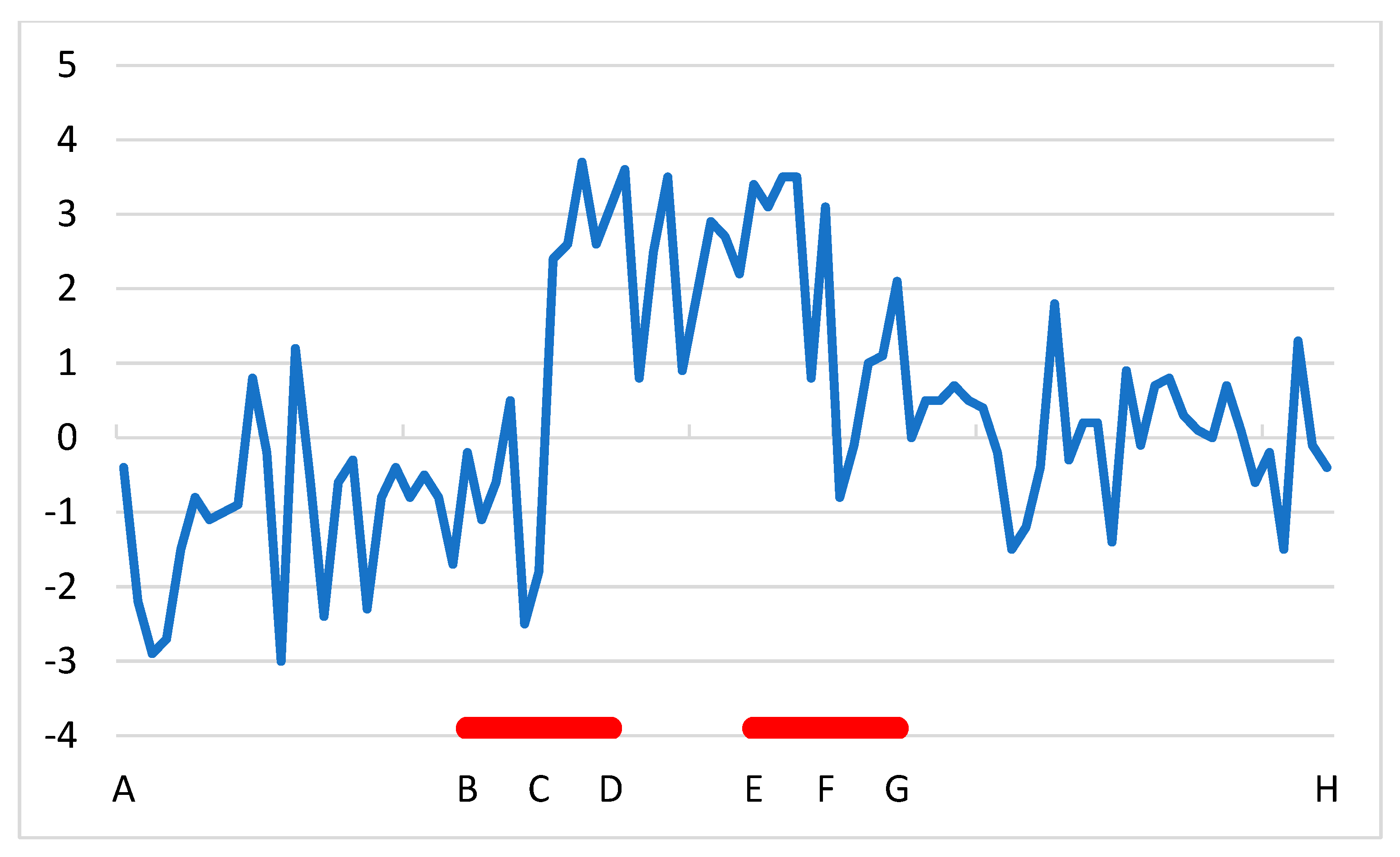
Often only relatively short sections of the time series are used in QM (marked with red color in Figure 2, and referred to as red sections). This results in increased sampling errors. In addition, only neighbor series with no detected break in the red sections of the time series are used, which may reduce further the amount of data considered, and may increase further sampling errors.

(ii)

Given that only neighbor series with no break in the red sections are used in the QM procedure related to the matching detected break of the candidate series, the sets of neighbor series considered often differ for different breaks. For instance, in Figure 2, neighbor series with no detected break between B and D are used in the calculations for break C, while neighbor series with no detected break between E and G are used in the calculations for break F. However, the expected value of estimations varies according to neighbor series, and thus the change in the set of neighbor series acts as if an unconsidered break was between D and E, affecting the overall bias between A and H.

(iii)

The omission of multiple break detection rules likely contributed to the low accuracy of the final results in the tests of [27,28,29].

The error types of (i) and (ii) cannot be avoided when the described QM algorithm is used. Therefore, although QM can give very good results in some case studies, it should not be included in automatic or semi-automatic methods of time series homogenization.

2.3. Climatol

The Climatol homogenization method [30,31] includes the standard normal homogeneity test [45] with binary segmentation [46] for break detection, and iteratively performed spatial interpolations for the removal of inhomogeneity biases. Spatial interpolation, by its nature, includes the consideration of the season of the year and the anomaly from the long-term mean. For this reason, Climatol includes the homogenization of probability distribution. Method comparison tests show that Climatol is one of the best presently available homogenization methods, and it is also a frequently applied method in practical homogenization [47,48,49,50,51,52,53]. Note, however, that Climatol has two weaknesses: this method cannot treat adequately regional mean biases [25], and the homogenized time series include area-average values (except for the last HSP of the time series), by which some station specific characteristics of the observed data are lost.

2.4. MASHv4

In the homogenization method MASH [14], the break detection is performed with multiple t-test, and inhomogeneity biases are removed iteratively according to the inbuilt test statistics of the method. The latest version, MASHv4 [54], includes the detection and bias removal for section mean variances. Although this development does not fully resolve the homogenization of probability distribution, it can be considered an important step forward. The previous version MASHv3 was examined by some method comparison tests [25,26,27]. The test results indicate that the performance of MASH is generally good, although weaker than those of ACMANT and Climatol. MASH is applied in practice mainly in Central Europe [35,55,56,57,58].

3. Homogenization of the Probability Distribution for Time Series (HPDTS)

I propose a new method, in which the results of the homogenization for section mean values, and also station specific characteristics of the time series are preserved, and inhomogeneity biases of the probability distribution are removed or at least reduced. The name of this method is Homogenization of the Probability Distribution for Time Series (HPDTS).

3.1. Principles of the Development

• The input dataset of the procedure comprises the homogenized time series obtained by the ACMANTv5.3 procedure. The time series are divided into intervals similarly to QM. The way of the division is fixed for any given climate variable. During the operations, the arithmetical mean or extreme values of the observed daily values within a given PDF interval are used.
• The HPDTS procedure is applied separately to each candidate series of a studied dataset, but each candidate time series is examined together with a set of neighbor series.
• A statistical significance test is performed for each break of the candidate series detected by ACMANTv5.3, and breaks being insignificant for HPD are skipped.
• All pieces of the candidate series and neighbor series data are used in the calculations, and the combined effect of inhomogeneities are calculated by an equation system similar to Benova.
• Symmetric low pass filters and linear interpolation between adjacent quantiles are applied, while the use of any other function type is avoided.
• HPDTS does not alter HSP means, so that all HSP means calculated by ACMANTv5.3 are preserved.
• In the version presented here, seasonal changes in inhomogeneity biases are not considered either in the ACMANTv5.3 procedure (seasonality mode “flat” is selected) or during HPDTS.

3.2. Concepts and Definitions

In the presentation of HPDTS algorithm the terminology of [21] is used. Here, the meanings of some specific terms and denotations are explained.

-

Homogenized period: the period of the time series for which homogenization can be performed, i.e., it has sufficient amount of observed data, and the period can be compared to the data of a sufficient number of neighbor series. This term can be applied either before or after the homogenization is executed.

-

Relative time series: series of differences between a candidate series and its neighbor series. In HPDTS the candidate series is compared to one composite reference series.

-

Station effect: the summarized effect of station representativeness and inhomogeneity biases. The station representativeness is a station specific constant, while inhomogeneity biases are approached by step function.

-

Style of symbols: scalars are written by italics, while vectors and matrix are presented by bold capital letters.

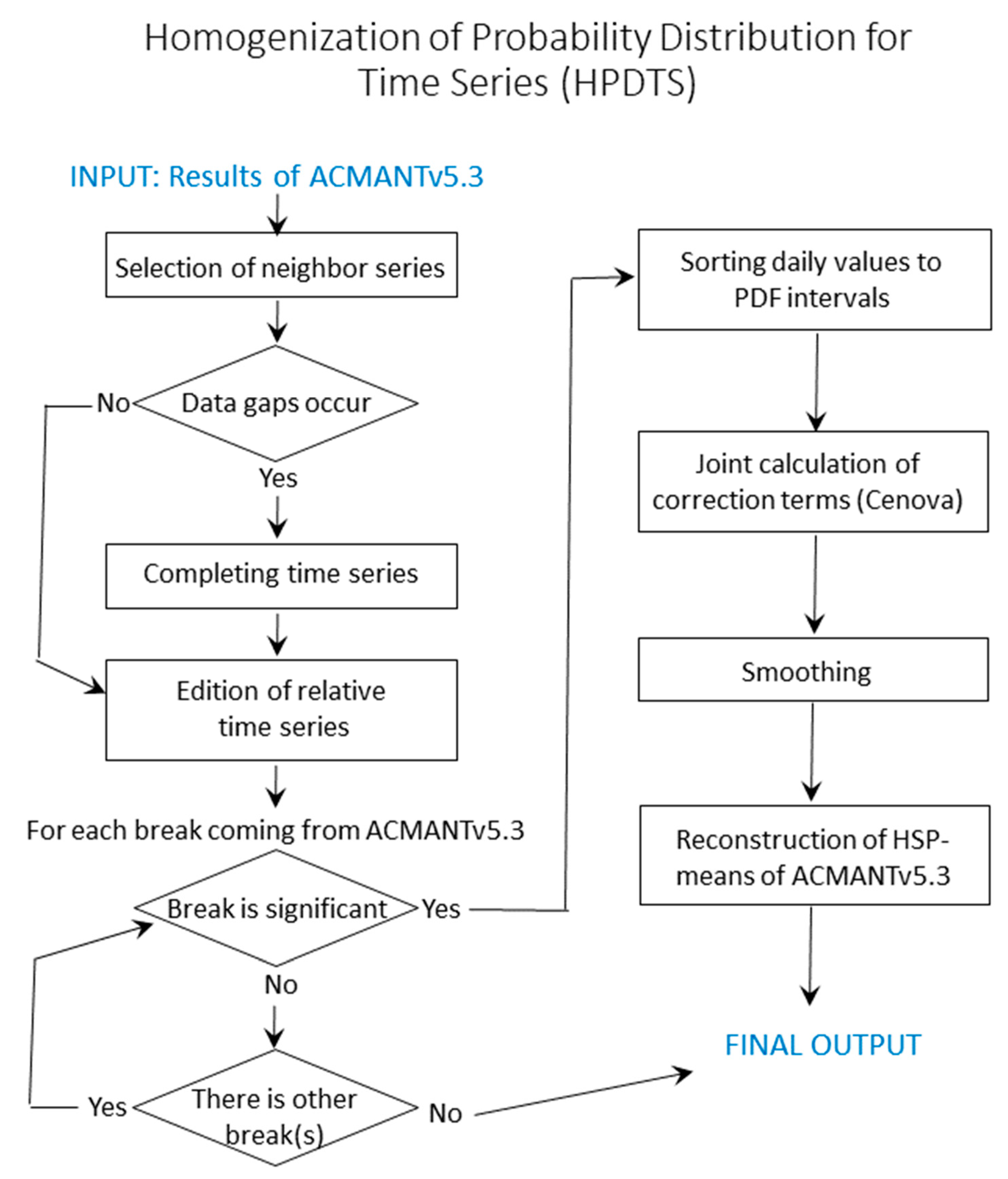
3.3. HPDTS Algorithm

The HPDTS algorithm is applied separately to each time series of the dataset. The actually examined time series is referred to as a candidate series.

Step 1. Neighbor series are selected to the candidate series according to the rank order of the spatial correlations (R) with the candidate series. Deseasonalized monthly increment series [21] are used for the calculation of R. Any neighbor series used by ACMANTv5.3 can be accepted to HPDTS, except for series with shorter than the 20 years homogenized period when the length of the homogenized period of the candidate series is at least the double of that of the neighbor series. In HPDTS the maximum number of neighbor series is 10, while when less than 3 neighbor series meet with the required conditions, no HPDTS is performed. Together with the candidate series, a network for HPDTS (hereafter: network) comprises N time series where 4 ≤ N ≤ 11. Note that these networks are often smaller than those of the previous ACMANTv5.3 procedure.

Step 2. Data gaps within the homogenized period of the candidate series are infilled in all series of the network. This includes that relatively short neighbor series are also completed to the homogenized period of the candidate series. The gap filling is performed similarly to step 20.4 of [21], and only in this step, time series out of the network may contribute to the procedure. There are two modifications relative to the gap filling procedure of 20.4 of [21]: (i) monthly data-pairs are used to calculate the candidate series – neighbor series relations (here, exceptionally, candidate series means the series for which gap filling is performed) also in daily data interpolation, which is a general change in ACMANTv5 relative to ACMANTv4; (ii) only in HPDTS: the candidate series of the HPDTS does not take part in the gap filling of any neighbor series.

Step 3. The minimum length of HSPs is elevated to 9 months both in the candidate series and the neighbor series. Shorter HSPs are preserved only for the candidate series when its spatial correlations with the first 6 neighbor series are ≥0.85. When an HSP is shorter than expected, one of its bordering breaks is canceled from the break list. The selection of the break to be dropped depends on the total length (L) of its connecting two HSPs (Equation (1)).

$$L=L_1+L_2$$

(1)

L₁ (L₂) stands for the length of the HSP on the left (right) side of the examined break. When a break must be dropped for the shortness of one of its connecting HSPs, always the one with the shortest L is canceled. The execution of this step is iterative, it starts with the exclusion of the break with the shortest L (but only when L₁ or L₂ is shorter than 9 months) and lasts until at least one HSP is shorter than 9 months.

Step 4. A relative time series of daily values (T) is created similarly to step 22.7.1 of [21], but here the relative time series covers the whole homogenized period of the candidate series. Note that in this procedure, T series are used only for testing the significance of breaks in HPD.

Step 5. Significance test for the breaks of the candidate series. The initial list of the breaks comes from the list of the detected breaks by ACMANTv5.3, so once they have passed a significance test. However, the significance for HPD may differ from the significance for homogenization of the section means, as it was illustrated in Figure 1. The basic idea of the significance test here is that when the inhomogeneity biases significantly differ for the tails of the PDF from the mean inhomogeneity bias, the differences between the T values of a tail from the average of T values must have the same sign. For instance, dividing the range of 0 to 0.2 of the PDF to the four subsections of 0–0.05, 0.05–0.1, 0.1–0.15 and 0.15–0.2, the deviations of these section means from the overall mean should be of the same sign. When both the ranges of 0 to 0.2 and 0.8 to 1 are divided into four subsections and all signs are the same within any given tail, the random chance that the break is insignificant (first type error) is only 1/2⁶. However, typical PDF distributions (Figure 1) show that inhomogeneity biases likely differ most at the most extreme sections, and thus random effects might influence more the test results for the subsections closer to the median than for the most extreme subsections. Therefore, in the significance test here, the four bins of a tail is constructed in a way that values both from the most extreme 0.1 wide interval and the less extreme 0.1 wide interval fall into any bin (Figure 3).

Then, the arithmetical averages and the differences from the overall mean are calculated for each bin. When the signs are the same only for the bins of one tail, one more test is performed for the T values at that tail. In this test, the range of 0 to 0.21 (or 0.79 to 1) of the PDF is divided into 14 subsections, and their values are sorted into seven bins in a similar way as the sorting into four bins was performed in the first test. The break is significant in this second test if all the seven signs of the differences from the overall mean are the same.

Once a break has been canceled for the lack of significance, the significance of the adjacent breaks might change. Therefore, the check of break significances is performed iteratively, starting from the break separating the HSPs of the shortest L.

Note 1: The division of PDF presented here is used only in the significance tests, and is the same for any climate element.

Note 2: Spatial correlations are left out of consideration in the significance tests, since a break can be significant in a way that the noise is high, but the sign is even higher (high dependence of inhomogeneity bias on PDF values), while it can be insignificant in a way that although the noise is low, the sign is even lower.

Step 6. From this step, HPDTS is similar to QM from the point of view that first the biases are calculated for a finite number of quantiles, then smoothers are applied; but the procedure differs from QM in editing and using an equation system similar to that of Benova for each pre-selected quantile. The modified Benova system is called Cenova. In this step, the number of synchronous breaks is controlled, as this is an obligatory preparatory step for applying any Benova-type equation system. The maximum number of breaks (N_TH) within any 9-month-long period is set by Formula (2).

$$N_{TH}\le N-3$$

(2)

When the number of synchronous breaks is higher than N_TH, the break separating the HSPs of the shortest L is canceled from the break list, and this step may be repeated if the remaining number of breaks is still higher than N_TH.

Step 7. The use of Cenova will need a continuous data field, and in this respect, a problem is that the occurrences of values falling into a given interval of the PDF are discontinuous in time. Therefore, sections of time series will be filled with the arithmetical mean of the data belonging to the actually examined PDF interval. At this step, the division to sections (HSP*) is specified. All HSP*s of the candidate series are identical with its homogeneous sub-periods. However, in neighbor series, the separating points between two adjacent HSP*s are not always breaks of the same series. More specifically: (i) the breaks of the candidate series are separating points in all neighbor series; (ii) any break closer than 5 months to a break of the candidate series is not a separating point; (iii) all breaks which are not excluded by (ii) are also separating points. (iv) Any section between two consecutive separation points is an HSP*.

Step 8. The empirical PDF of the input data (x) of HSP* sections are divided to subjectively defined P intervals for each HSP* of each time series. The intervals tend to be longer than average around the maximum of the frequency distribution and shorter for ranges of rare extreme values. In this study, the following divisions of the PDF are applied: (i) for wind speed, P = 9, and the threshold values of PDF intervals are 0, 0.1, 0.25, 0.4, 0.6, 0.75, 0.85, 0.9, 0.95 and 1; (ii) for relative humidity P = 10, and equidistant 0.1 long intervals are applied.

From this point, the intervals of the PDF are examined individually. The arithmetical mean of the values corresponds to the examined PDF interval and actual HSP* (x’) substitutes x in each day of the Cenova time series. The mean and extreme values for a given PDF interval and given HSP of the candidate series are preserved for later operations, and they will be referred to as distinguished points.

Step 9. The estimated regional mean climate signal ($\overline{u\prime }$) is extracted from each daily data x’, its reason will be explained in step 10. The regional mean climate is estimated by the 9-year moving average (MA) of the network mean x’ values (Equations (3) and (4)).

$$\overline{{u^{\prime }}_{y,d}}={\displaystyle \frac{1}{n^{*}{\sum }_{s=1}^N{w}_s}}{\sum }_{i=\max (1,y-4)}^{\min (n,y+4)}{\sum }_{d=1}^{365}{\sum }_{s=1}^N{w}_s{x}_{s,i,d}^{\prime }$$

(3)

$$x_{s,y,d}^{*}=x_{s,y,d}^{\prime }-\overline{{u^{\prime }}_{y,d}} \mathrm{for}\mathrm{every}s, y, d$$

(4)

Denotations: n—number of years in the study period; n*—number of daily data in the period of MA; y and d are year and day of the year, respectively; w—weight of time series. For the candidate series (s = 1) w₁ = 1, while for the neighbor series (s = 2,…N), the weights are the squared spatial correlations with the candidate series ($w_s=R_s^2$). Equation (3) shows that the periods considered in the MA are shorter at the tails of the study period.

Step 10. Calculation of the inhomogeneity biases by Cenova for all x’ values of the candidate series. The same kind of equation system is constructed as for Benova: here, the matrix of X* stands in the place of the observed data, while the list of the breaks is identical to the list of the detected breaks by ACMANTv5.3. Differences from the Benova method come from the performed manipulations (X → X*) of the input data. The Cenova equation system can be described by (5) and (6), where (5) is performed for each HSP of each series, and (6) is performed for each time unit (i), which is day in the present application.

$${\displaystyle \frac{1}{j_{s,k+1}-j_{s,k}}}{\sum }_{i=j_{s,k}+1}^{j_{s,k+1}}(\widehat{u_{s,i}}+u_{s,i}^{*})+\widehat{v_{s,k}}=\overline{{\mathbf{x}}_{\mathbf{s},\mathbf{k}}^{\mathbf{*}}}$$

(5)

$${\sum }_{s=1}^N{w}_s(\widehat{u_{s,i}}+u_{s,i}^{*})+{\sum }_{s=1}^N{w}_s\widehat{v_{s,k\left(i\right)}}={\sum }_{s=1}^N{w}_s{x}_{s,i}^{*}$$

(6)

In Equations (5) and (6), u and v denote climate signal and station effect, respectively; k and j stand for the serial number of break and the timing of break, respectively; and cap over symbols indicates estimated variable. The other symbols are used with the same meaning as in the previous equations. The difference from the weighted version of the Benova equations [20] is that the climate signal estimation is perturbed by u*(s,i). The deviation for this perturbation can be large when the HSP*s of neighbor series from which their HSP* means (x’) are calculated stretch far over the endpoints of the actually examined HSP. This cannot happen with the HSPs of the candidate series, because the breaks of the candidate series are included as separation points in all of its neighbor series. However, the results for the candidate series are also affected, due to the interdependence between the accuracies of individual estimations.

The deviations caused by the presence of U* in the equations tend to be larger when the climate signal includes notable trends or low frequency variations. That is why the low-frequency part of the estimated network mean climate signal was removed in step 9. In both Benova and Cenova, the network mean climate signal is neutral to the break size estimations except for changes in U* in Cenova. The estimations from X’ are acceptable, since the dataset was previously homogenized by ACMANTv5.3.

The results of this step is the first estimations of adjustment terms for the means of the observed values (x’) for intervals p = 1,2,…P, they are denoted by a₁, a₂,… a_P.

Step 11. Smoothing between adjacent adjustment terms of A. Weighted moving average (WMA) is applied according to Equation (7).

$$b_p={0.25\ast a}_{p-1}+0.5\ast a_p+{0.25\ast a}_{p+1}\mathrm{for} 1<p<P$$

(7)

b₁ = a₁;  b_P = a_P

Step 12. Calculation of the adjustment terms e for the lower threshold of PDF intervals. These adjustment terms are estimated by averaging the adjustment terms a for the adjacent PDF intervals, and extending the application of WMA to these distinguished points (Equation (8)).

$$e_p={0.125\ast a}_{p-2}+0.375\ast a_{p-1}+0.375\ast a_p+{0.125\ast a}_{p+1} \mathrm{for} 2<p<P$$

(8)

$$e_p={0.5\ast a}_{p-1}+0.5*a_p \mathrm{for} p=2\mathrm{and} p=P$$

e₁ = a₁; e_P+1 = a_P

Note 1. e_p+1 adjustment term is valid also for the upper threshold of interval p.

Note 2. A and E together comprise the adjustment terms for the distinguished points of the candidate series.

Step 13. Calculation of adjustment terms for all data points, and execution of adjustments. For any piece of data of the input time series (x), the adjustment term (q) is calculated by linear interpolation between the adjustment terms for the closest distinguished points. From them, the adjusted data (h’) are calculated (Equation (9)), but they are still not the final results.

$$h_{y,d}^{\prime }=x_{y,d}+q_{y,d} \mathrm{for} \mathrm{every} y \mathrm{and} d$$

(9)

Step 14. Reconstruction of the HSP means of the input time series. The most accurate estimation of HSP means is provided by the homogenization of section means. Therefore, when a HPD procedure modifies HSP means (for random errors of the procedure), such alterations must be revoked. It can be solved by adding a small correction to each daily data of the HSP (generally only small corrections are needed, which are hardly perceptible at the level of daily data). For instance, when a HSP mean in series h’ is higher with ∆ than the same HSP in series x, the correct HSP mean for the final homogenized series h can be reconstructed by Equation (10).

$$h_{y,d}=h_{y,d}^{\prime }-∆ \mathrm{for} \mathrm{every} y \mathrm{and}d \mathrm{within} \mathrm{the} \mathrm{HSP}$$

(10)

In Figure 4, the main steps of HPDTS are illustrated in a flowchart.

4. Efficiency of HPDTS

4.1. Test Dataset

The test datasets used in this study are a part of the benchmark dataset developed during the European project INDECIS (2017–2020). The benchmark dataset was created to test homogenization methods on synthetically constructed, but realistic, climate time series. The time series of the datasets are of daily resolution, and they include nonlinear inhomogeneities [31]. The homogeneous part of the benchmark was developed for nine climatic variables from model (reanalysis) data [59] for Sweden and Slovenia. Then, inhomogeneities were introduced to them to obtain the inhomogeneous datasets. The Swedish (Slovenian) network comprises 100 (30) time series for each climate variable. All the time series are 56-year long (1950–2005). The inhomogeneous dataset has a complete version (CO) and another with data gaps (DG) in the time series.

In this study, the datasets of wind speed and relative humidity are used. Both the Swedish and Slovenian networks, and both the CO and DG versions are tested with the newly developed ACMANTv5.3 + HPDTS method (referred to as A + HPDTS). In the DG versions, the mean ratio of missing data for individual datasets varies from 13.1% to 14.6% in the selected four datasets.

Before the actual test results will be shown in Section 4.2 and Section 4.3, here some details of the earlier results produced during INDECIS are recalled focusing on the RMSE of daily data and trend bias errors. During INDECIS, the benchmark was tested by three methods: ACMANT, Climatol and DAP [11]. In most test experiments, the daily RMSE of the inhomogeneous series was reduced only by 0 to 15% (by 20 to 30% in the most successful cases) by any homogenization method, and this was true for all of the nine tested climate variables [29]. By contrast, ACMANT and Climatol removed large parts of the trend bias errors. These results indicate the difficulty to achieve high daily data accuracy for this benchmark. Note that much better daily data accuracy (60% to 80% RMSE reduction) was achieved for the daily temperature benchmark dataset of [27] both with ACMANT and Climatol, but given that the present HPDTS version does not consider seasonality for inhomogeneity biases, temperature datasets are not used in this study.

One factor that may explain the weak results for INDECIS datasets is that the spatial correlations between daily data are relatively low (Figure 5). Correlations for daily data were calculated similarly to R, but taking the daily increment series instead of the monthly increment series.

The average of the five highest monthly correlations and that of the five highest daily correlations for any candidate series were used in the calculations for Figure 5. The curves of monthly correlations peak around 0.8, except for the Slovenian wind data where the monthly correlations are weaker. The correlations for daily series are much lower than for monthly series for relative humidity series, while this type difference is much smaller for the wind speed series. The curves of correlations for daily data peak around 0.60–0.65, except for the Swedish wind speed series, where the daily correlations are generally higher.

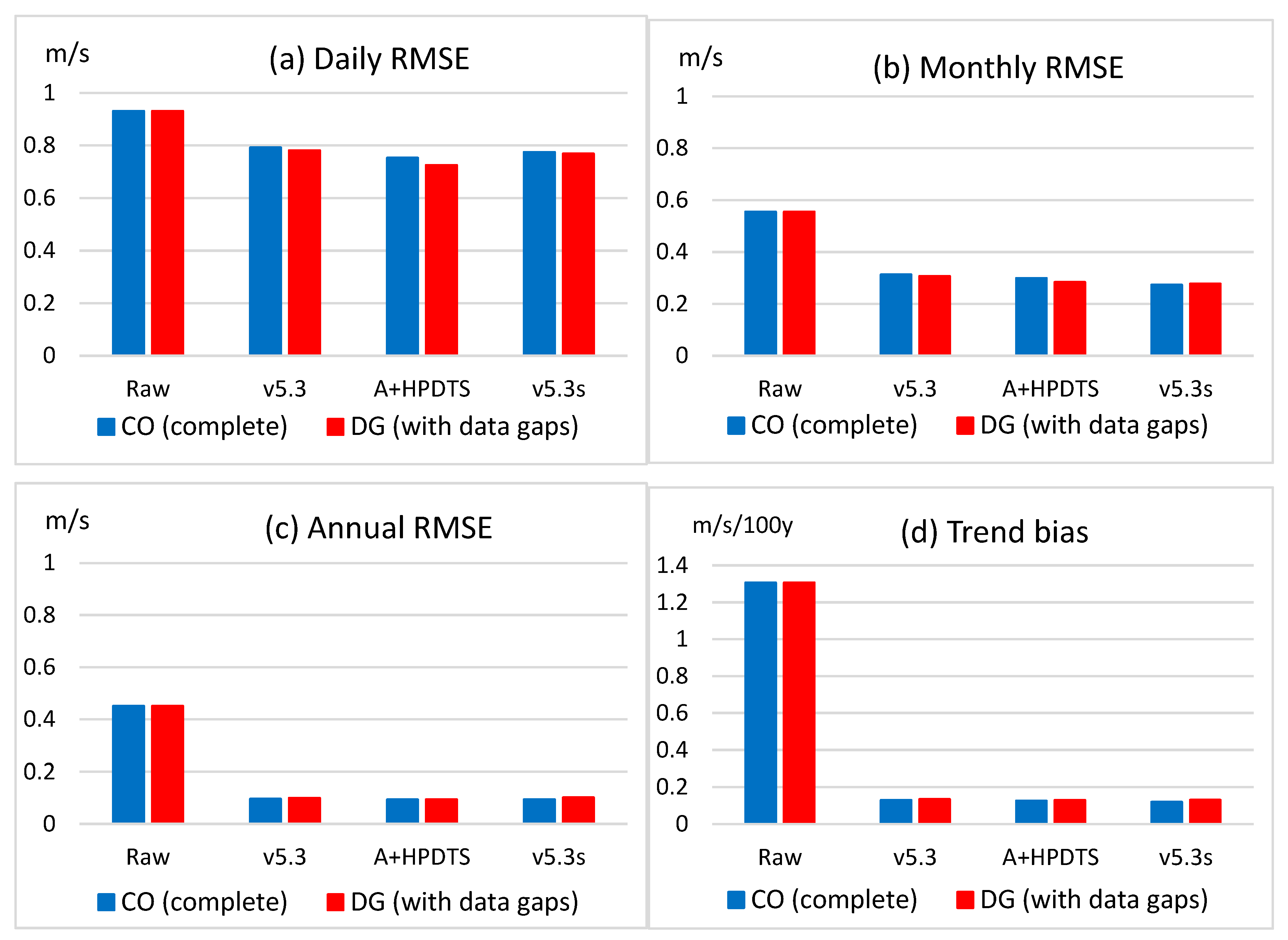
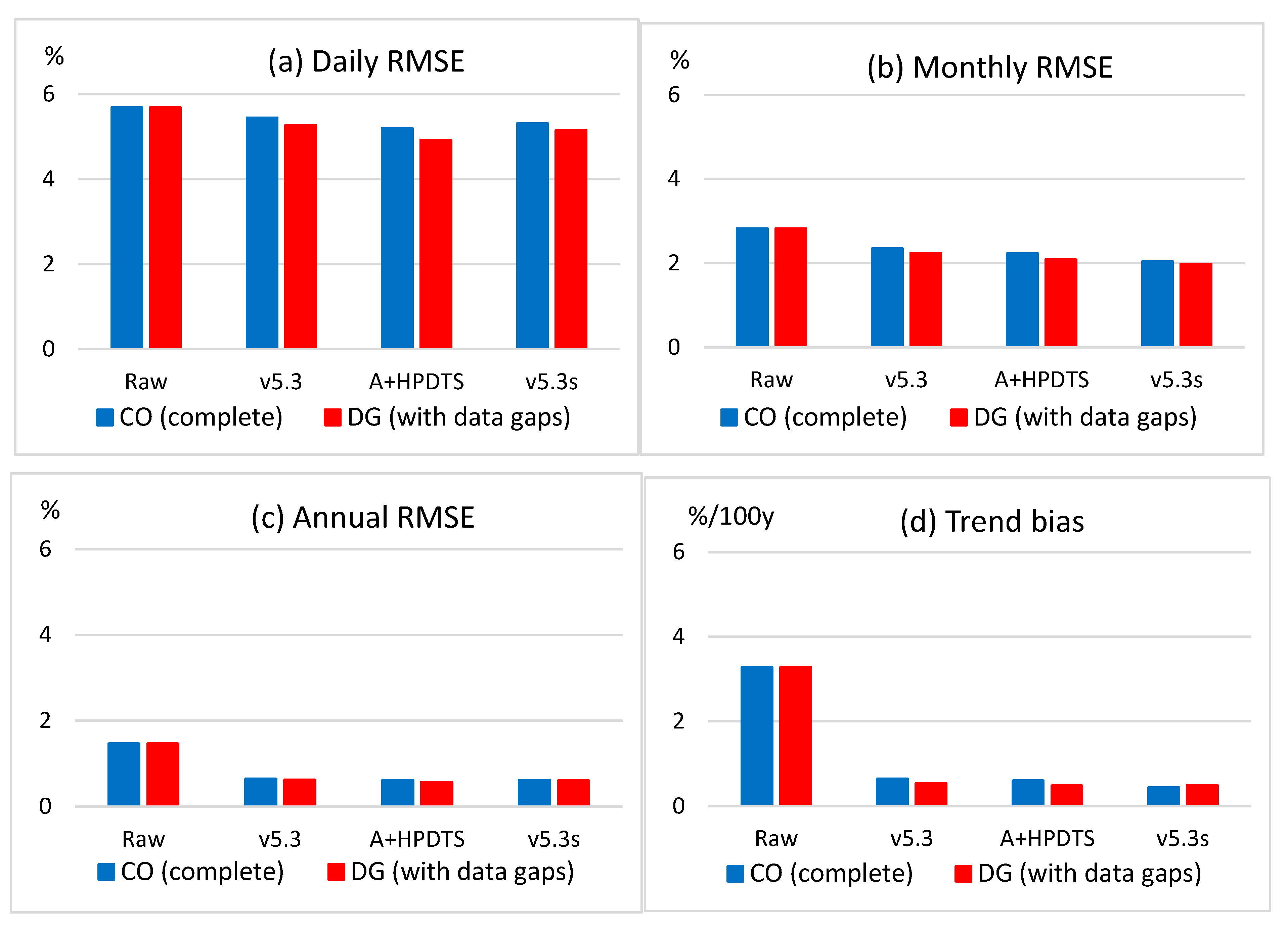
4.2. Test Results I: RMSE for All Data

Four error measures are used for presenting the efficiency of the proposed homogenization method of A + HPDTS: (a) RMSE of daily values; (b) RMSE of monthly values; (c) RMSE of annual values; (d) mean of absolute trend biases. Trend bias errors are calculated only to check if HPDTS preserves the good results of the ACMANT procedure for this error type. All types of errors are calculated for entire time series, and they are averaged for the individual datasets described in Section 4.1. In the calculations for DG datasets, still entire time series are evaluated, and interpolated data are treated in the same way as homogenized observed data. The homogenization results of HPDTS is compared with (i) raw data errors; (ii) ACMANTv5.3 without seasonality of inhomogeneity biases; (iii) ACMANTv5.3 with the inclusion of irregular seasonality of inhomogeneity biases (referred to as v5.3s).

Figure 6 shows the results for the Swedish wind speed datasets. With any of the tested homogenization methods, the error reduction is the highest for the trend bias errors, then the order of efficiency is annual RMSE reduction, monthly RMSE reduction and daily RMSE reduction. These kinds of differences in the homogenization efficiency are caused by the differing signal-to-noise ratios in the reduction in different error types, and are in line with the results of other efficiency tests [10,25,26,27,28,29]. Figure 6 shows that the largest RMSE reduction for daily data is obtained with the A + HPDTS method, and the inclusion of HPDTS also reduces the monthly RMSE. Regarding the annual RMSE and mean absolute trend bias, a major part of these errors are removed by ACMANTv5.3, and HPDTS preserves the good results. Surprisingly, the error reductions are slightly larger for the DG datasets than for the complete datasets.

Figure 7 shows the results for the Slovenian wind speed data. The results are rather similar to those of the Swedish wind speed homogenization, but here, the error reduction for daily RMSE is lower with each of the tested methods. In comparing the results of the individual methods, A + HPDTS is again the most efficient, and the results for the DG dataset are again better than those for the complete dataset.

Figure 8 shows the results for the Swedish relative humidity datasets. For this climate element the error reduction is generally less successful than for wind speed with any of the tested methods. In the reduction for daily RMSE, A + HPDTS produces little improvement, yet it still gives the best results among the tested methods, while for monthly RMSE the error reduction is the highest with v5.3s. Regarding the annual RMSE and mean absolute trend bias, large parts of the raw data errors are also removed with any of the tested methods for this variable.

Figure 9 shows the results for the Slovenian relative humidity datasets. The results are similar to the ones shown in the previous figures, although the error reductions presented here are somewhat larger than those for the Swedish relative humidity data. In the results of Figure 9, the differences between CO and DG results are higher than in the previously presented results (Figure 6, Figure 7 and Figure 8), and the error reduction is consequently larger for the dataset with data gaps. Here, the monthly RMSE reduction is clearly larger with v5.3s than with A + HPDTS.

Table 1. Reduction in RMSE and mean absolute trend bias errors (percentage) by the inclusion of HPDTS in the homogenization with ACMANT. CO—complete series, DG—series with data gaps, FF—wind speed, HH—relative humidity, Sw—Sweden, Sl—Slovenia. Negative values indicate increase in errors.

	Daily RMSE		Monthly RMSE		Annual RMSE		Trend Bias
	CO	DG	CO	DG	CO	DG	CO	DG
FF_Sw	8.7	10.6	8.9	11.4	9.3	12.0	4.8	0.9
FF_Sl	4.9	7.2	4.6	7.3	3.9	5.2	2.9	3.4
HH_Sw	4.6	6.5	4.8	7.0	5.0	8.5	6.9	9.8
HH_Sl	5.0	10.1	5.1	9.6	5.0	7.5	–0.6	–0.7

summarizes the error reductions achieved by the inclusion of HPDTS in the homogenization with ACMANT.

In Table 1, the ratios of error reduction for highly differing absolute errors can more easily be compared than in Figure 6, Figure 7, Figure 8 and Figure 9. Interestingly, the RMSE reduction in different time scales is almost uniform when the ratios are considered, and they are consequently higher for the DG datasets than the CO datasets. The homogenization was the most successful for the Swedish wind speed datasets, where the RMSE reduction is 9% (10–12%) in all time scales for the CO (DG) dataset, while in the other cases, the RMSE reduction is only 4–5% (5–10%) for the CO (DG) datasets. The homogenization slightly reduced the mean absolute trend bias (except for the Slovenian relative humidity datasets), but the changes found are insignificant, because trend bias errors within a given dataset are not statistically independent, and thus the random component of the calculated trend bias errors is relatively high.

4.3. Test Results: RMSE for Extreme Values

Table 2. RMSE and its reduction by HPDTS and by the complete homogenization procedure of ACMANTv5.3 + HPDTS. Two extreme ranges (f < 0.05 and f > 0.95) of the probability distribution function are examined. CO—complete series, DG—series with data gaps, FF—wind speed, HH—relative humidity, red. by HPDTS—error reduction in comparison to the ACMANTv5.3 results, error reduction total—error reduction in A + HPDTS in comparison to the raw data errors. Highest (lowest) error reductions are enhanced by bold (italics). Negative values indicate increase in errors.

	Sweden				Slovenia
	f < 0.05		f > 0.95		f < 0.05		f > 0.95
	CO	DG	CO	DG	CO	DG	CO	DG
FF RMSE (m/s)	0.6	0.6	0.9	1.0	0.5	0.6	1.3	1.3
FF red. by HPDTS (%)	1.5	–0.8	8.5	9.1	1.5	–1.5	4.2	3.9
FF error reduction total	13.5	5.6	31.0	29.9	–4.2	–11.7	18.2	18.2
HH RMSE (%)	7.5	7.1	2.9	3.0	10.3	9.8	3.6	3.7
HH red. by HPDTS (%)	3.7	4.5	0.3	–1.1	3.9	4.6	–1.3	–4.0
HH error reduction total	7.6	12.0	0.2	–4.6	10.4	14.9	1.4	–1.5

shows some homogenization results for the two extreme 5% wide ranges of the probability distribution. The homogenized daily RMSE by A + HPDTS method and the RMSE reductions by HPDTS and A + HPDTS methods are presented.

The RMSE reduction by HPDTS is successful for the extreme high wind speed and extreme low relative humidity values, while the application of HPDTS does not improve the accuracy for extremely low wind speeds and extremely high relative humidity values. Note, however, that the absolute RMSE are the lowest for extreme low wind speeds (where the observed values are close to 0) and for extreme high relative humidity values (observed values are close to 100%). The notable error reduction for extreme high wind speeds (30–31% by A + HPDTS) is particularly valuable for the enhanced practical importance of their accuracy.

Table 2 also shows that the presence of data gaps increases the risk of the worsening of data accuracy at the extreme ranges of the PDF when HPDTS is applied, although the degree of such worsening is insignificant.

5. Discussion

The proposed HPDTS method produced a moderate RMSE reduction (4–12%) for the daily data of the tested datasets, and the results for the extreme ranges are partly even weaker. These facts may suggest that HPDTS has a moderate efficiency, but the following factors should be considered in a profound evaluation: (i) the spatial correlations within the used test datasets are moderate, except for the Swedish wind speed datasets; (ii) in earlier tests, very little improvement in daily data accuracy was produced with any homogenization method [29]; (iii) the results presented here indicate that the daily data accuracy increases with increasing spatial correlations; (iv) the inclusion of HPDTS in ACMANT improves data accuracy in all time scales, and does not affect the accuracy of trend bias estimations; (v) when the spatial correlations are moderate, although only little accuracy improvement can be produced, but the risk of worsening data accuracy is still very low, which is a big step forward in comparison to [44].

The tests with HPDTS gave less stable results for the extreme ranges than for the mean RMSE. In the interpretation of the results, the following factors should be considered: (i) a symmetric low pass filter was applied for all intervals of the PDF, except for the extreme tails where its use is impossible; therefore, a certain weakening of the efficiency for the extreme ranges is likely; (ii) breaks with statistical significant biases only in one of the extreme tails of the PDF may pass the significance test, and in this case, the risk of producing spurious adjustments at the other tail of the PDF is elevated.

One surprising feature of the test results is that the RMSE reduction by HPDTS was generally higher for datasets with 13–15% missing data ratio than for complete datasets. Given that the only difference between the CO and DG datasets are the presence of data gaps in the latter ones, the only possible explanation is that the RMSE reducing effect of data averaging by spatial interpolations exceeds the direct impact of missing data on the data accuracy. Nevertheless, the use of interpolated data will not be widened in ACMANT for the following reasons: (i) spatially interpolated data have partly different properties in comparison to homogenized station specific data series, and the results for the extreme ranges (Table 2) indicate that the error reduction by spatial averaging does not extend to all statistical properties; (ii) for users preferring the use of regional averages, gridded datasets are available.

To consider the common effect of individual inhomogeneities in the phase of the data correction, an alternative version of the Benova equation system [20], referred to as Cenova, is applied in HPDTS. Note that Cenova might give bad results when the regional climate signal includes strong trends or other kinds of low frequency changes. In the present Cenova application, the regional mean climate signal was removed by estimating the climate signal from the previously homogenized input dataset.

In the network construction for HPDTS, only the rank order of spatial correlations is considered (except for special cases specified in Step 1 of Section 3.3), and all time series are completed to the homogenized period of the candidate series. This means that a high portion of neighbor series data may originate from spatial interpolations. This is allowed in HPDTS, because the interpolations are performed using data previously homogenized by ACMANTv5.3.

The development of HPDTS method is a part of the dataset development project of the Catalan Meteorological Service, and a part of the development of the future version ACMANTv6. The research will be continued by addressing the seasonal variations in inhomogeneity biases. The presented results show that the consideration of such seasonal variations tends to improve the accuracy of monthly values, and the joint consideration of the dependence of inhomogeneity biases on quantiles of the PDF and seasonality may improve further the data accuracy. Another issue for studying in the future is the possible inclusion of breaks for section mean variances [54,60,61] in HPDTS. The present form of HPDTS presumes that the significant breaks for homogenizing probability distribution have already been detected by the step function fitting steps of the ACMANTv5.3 procedure. While significant inhomogeneities of PDF often go together with significant inhomogeneities of the means, exceptions occur [62].

6. Conclusions

The HPDTS (Homogenization of Probability Distribution for Time Series) method has been developed to improve the accuracy of observed climatic data, and enhance their usability in climate studies and applied climatic studies.

• HPDTS is applied on datasets for which the section mean biases have been removed by a previous homogenization procedure.
• HPDTS considers the joint effect of inhomogeneity biases by calculating all adjustment terms with an equation system (Cenova) summarizing the climate signal and station effects within a given network. Using this method, the accuracy of daily and monthly data are improved, and the positive features of the previous homogenization results are preserved.
• HPDTS applies adjustments only for breaks which cause significant quantile dependent inhomogeneity biases.
• The present version of the method does not consider seasonal variations in inhomogeneity biases.
• HPDTS has been tested on some sections of the European project INDECIS benchmark dataset, and the test results are favorable. HPDTS resulted in 4 to 12% RMSE reduction in wind speed and relative humidity test data in all temporal scales. The results for the extreme tails of the PDF were more varied, but the notable accuracy improvement of high wind speed data is highlighted here for the great practical importance of this type of climatic extremes.

References

1. Auer, I.; Böhm, R.; Jurkovic, A.; Orlik, A.; Potzmann, R.; Schöner, W.; Ungersböck, M.; Brunetti, M.; Nanni, T.; Maugeri, M.; et al. A new instrumental precipitation dataset for the Greater Alpine Region for the period 1800–2002. Int. J. Climatol. 2005, 25, 139–166. [Google Scholar] [CrossRef]
2. Venema, V.; Trewin, B.; Wang, X.L.; Szentimrey, T.; Lakatos, M.; Aguilar, E.; Auer, I.; Guijarro, J.; Menne, M.; Oria, C.; et al. Guidelines on Homogenization; WMO-No. 1245; World Meteorological Organization: Geneva, Switzerland, 2020. [Google Scholar]
3. Trewin, B. A daily homogenized temperature data set for Australia. Int. J. Climatol. 2013, 33, 1510–1529. [Google Scholar] [CrossRef]
4. Brunet, M.; Asin, J.; Sigró, J.; Bañon, M.; García, F.; Aguilar, E.; Palenzuela, J.E.; Peterson, T.C.; Jones, P. The minimization of the screen bias from ancient Western Mediterranean air temperature records: An exploratory statistical analysis. Int. J. Climatol. 2011, 31, 1879–1895. [Google Scholar] [CrossRef]
5. Hannak, L.; Friedrich, K.; Imbery, F.; Kaspar, F. Analyzing the impact of automatization using parallel daily mean temperature series including breakpoint detection and homogenization. Int. J. Climatol. 2020, 40, 6544–6559. [Google Scholar] [CrossRef]
6. Vicente-Serrano, S.M.; Beguería, S.; López-Moreno, J.I.; García-Vera, M.A.; Stepanek, P. A complete daily precipitation database for northeast Spain: Reconstruction, quality control, and homogeneity. Int. J. Climatol. 2010, 30, 1146–1163. [Google Scholar] [CrossRef]
7. Domonkos, P.; Tóth, R.; Nyitrai, L. Climate Observations: Data Quality Control and Time Series Homogenization; Elsevier: Amsterdam, The Netherlands, 2022; 302p. [Google Scholar]
8. Domonkos, P. Relative homogenization of climatic time series. Atmosphere 2024, 15, 957. [Google Scholar] [CrossRef]
9. Menne, M.J.; Williams, C.N.; Vose, R.S. The U.S. Historical Climatology Network Monthly Temperature Data, Version 2. Bull. Am. Meteor. Soc. 2009, 90, 993–1008. [Google Scholar] [CrossRef]
10. Venema, V.; Mestre, O.; Aguilar, E.; Auer, I.; Guijarro, J.A.; Domonkos, P.; Vertacnik, G.; Szentimrey, T.; Štěpánek, P.; Zahradníček, P.; et al. Benchmarking monthly homogenization algorithms. Clim. Past 2012, 8, 89–115. [Google Scholar] [CrossRef]
11. Štěpánek, P.; Zahradnicek, P.; Farda, A. Experiences with data quality control and homogenisation of daily records of various meteorological elements in the Czech Republic in the period 1961–2010. Időjárás 2013, 117, 123–141. [Google Scholar]
12. Lindau, R.; Venema, V.K.C. The uncertainty of break positions detected by homogenization algorithms in climate records. Int. J. Climatol. 2016, 36, 576–589. [Google Scholar] [CrossRef]
13. O’Neill, P.; Connolly, R.; Connolly, M.; Soon, W.; Chimani, B.; Crok, M.; de Vos, R.; Harde, H.; Kajaba, P.; Nojarov, P.; et al. Evaluation of the homogenization adjustments applied to European temperature records in the Global Historical Climatology Network Dataset. Atmosphere 2022, 13, 285. [Google Scholar] [CrossRef]
14. Szentimrey, T. Multiple Analysis of Series for Homogenization (MASH). In Second Seminar for Homogenization of Surface Climatological Data; Szalai, S., Szentimrey, T., Szinell, C., Eds.; WCDMP-41; WMO: Geneva, Switzerland, 1999; pp. 27–46. [Google Scholar]
15. Szentimrey, T. Methodological questions of series comparison. In Sixth Seminar for Homogenization and Quality Control in Climatological Databases; Lakatos, M., Szentimrey, T., Bihari, Z., Szalai, S., Eds.; WCDMP-76; WMO: Geneva, Switzerland, 2010; pp. 1–7. [Google Scholar]
16. Caussinus, H.; Mestre, O. Detection and correction of artificial shifts in climate series. J. R. Stat. Soc. Ser. C Appl. Stat. 2004, 53, 405–425. [Google Scholar] [CrossRef]
17. Mestre, O.; Domonkos, P.; Picard, F.; Auer, I.; Robin, S.; Lebarbier, E.; Böhm, R.; Aguilar, E.; Guijarro, J.; Vertacnik, G.; et al. HOMER: Homogenization software in R—Methods and applications. Időjárás 2013, 117, 47–67. [Google Scholar]
18. Menne, M.J.; Williams Jr, C.N. Homogenization of temperature series via pairwise comparisons. J. Clim. 2009, 22, 1700–1717. [Google Scholar] [CrossRef]
19. Lindau, R.; Venema, V.K.C. On the reduction of trend errors by the ANOVA joint correction scheme used in homogenization of climate station records. Int. J. Climatol. 2018, 38, 5255–5271. [Google Scholar] [CrossRef]
20. Domonkos, P.; Joelsson, L.M.T. ANOVA (Benova) correction in relative homogenization: Why it is indispensable. Int. J. Climatol. 2024, 44, 4515–4528. [Google Scholar] [CrossRef]
21. Domonkos, P. ACMANTv4: Scientific Content and Operation of the Software. 2020, 71p. Available online: https://github.com/dpeterfree/ACMANT/blob/ACMANTv4.4/ACMANTv4_description.pdf (accessed on 6 April 2024).
22. Domonkos, P. Combination of using pairwise comparisons and composite reference series: A new approach in the homogenization of climatic time series with ACMANT. Atmosphere 2021, 12, 1134. [Google Scholar] [CrossRef]
23. Joelsson, L.M.T.; Sturm, C.; Södling, J.; Engström, E.; Kjellström, E. Automation and evaluation of the interactive homogenization tool HOMER. Int. J. Climatol. 2022, 42, 2861–2880. [Google Scholar] [CrossRef]
24. Bock, O.; Collilieux, X.; Guillamon, F.; Lebarbier, E.; Pascal, C. A breakpoint detection in the mean model with heterogeneous variance on fixed time-intervals. Stat. Comput. 2020, 30, 195–207. [Google Scholar] [CrossRef]
25. Domonkos, P.; Guijarro, J.A.; Venema, V.; Brunet, M.; Sigró, J. Efficiency of time series homogenization: Method comparison with 12 monthly temperature test datasets. J. Clim. 2021, 34, 2877–2891. [Google Scholar] [CrossRef]
26. Guijarro, J.A.; López, J.A.; Aguilar, E.; Domonkos, P.; Venema, V.K.C.; Sigró, J.; Brunet, M. Homogenization of monthly series of temperature and precipitation: Benchmarking results of the MULTITEST project. Int. J. Climatol. 2023, 43, 3994–4012. [Google Scholar] [CrossRef]
27. Killick, R.E. Benchmarking the Performance of Homogenisation Algorithms on Daily Temperature Data. Ph.D. Thesis, University of Exeter, Exeter, UK, 2016. Available online: https://ore.exeter.ac.uk/repository/handle/10871/23095 (accessed on 16 May 2025).
28. Guijarro, J.A. Recommended Homogenization Techniques Based on Benchmarking Results. WP-3 Report of INDECIS Project. 2019. Available online: http://www.indecis.eu/docs/Deliverables/Deliverable_3.2.b.pdf (accessed on 6 April 2024).
29. INDECIS-WP3 Benchmarking Results. 2019. Available online: https://github.com/dpeterfree/INDECIS/blob/main/INDECIS-WP3_benchmarking_results.pdf. (accessed on 23 March 2025).
30. Guijarro, J.A. Homogenization of Climatic Series with Climatol. 2018. Available online: https://www.climatol.eu (accessed on 6 April 2024).
31. Skrynyk, O.; Aguilar, E.; Guijarro, J.; Randriamarolaza, L.Y.A.; Bubin, S. Uncertainty evaluation of Climatol’s adjustment algorithm applied to daily air temperature time series. Int. J. Climatol. 2021, 41, E2395–E2419. [Google Scholar] [CrossRef]
32. Yosef, Y.; Aguilar, E.; Alpert, P. Changes in extreme temperature and precipitation indices: Using an innovative daily homogenized database in Israel. Int. J. Climatol. 2019, 39, 5022–5045. [Google Scholar] [CrossRef]
33. Fioravanti, G.; Piervitali, E.; Desiato, F. A new homogenized daily data set for temperature variability assessment in Italy. Int. J. Climatol. 2019, 39, 5635–5654. [Google Scholar] [CrossRef]
34. Adeyeri, O.E.; Laux, P.; Ishola, K.A.; Zhou, W.; Balogun, I.A.; Adeyewa, Z.D.; Kunstmann, H. Homogenising meteorological variables: Impact on trends and associated climate indices. J. Hydrol. 2022, 607, 127585. [Google Scholar] [CrossRef]
35. Chimani, B.; Bochníček, O.; Brunetti, M.; Ganekind, M.; Holec, J.; Izsák, B.; Lakatos, M.; Tadić, M.P.; Manara, V.; Maugeri, M.; et al. Revisiting HISTALP precipitation dataset. Int. J. Climatol. 2023, 43, 7381–7411. [Google Scholar] [CrossRef]
36. Prohom, M.; Domonkos, P.; Cunillera, J.; Barrera-Escoda, A.; Busto, M.; Herrero-Anaya, M.; Aparicio, A.; Reynés, J. CADTEP: A new daily quality-controlled and homogenized climate database for Catalonia (1950–2021). Int. J. Climatol. 2023, 43, 4771–4789. [Google Scholar] [CrossRef]
37. Molina-Carpio, J.; Rivera, I.A.; Espinoza-Romero, D.; Cerón, W.L.; Espinoza, J.-C.; Ronchail, J. Regionalization of rainfall in the upper Madeira basin based on interannual and decadal variability: A multi-seasonal approach. Int. J. Climatol. 2023, 43, 6402–6419. [Google Scholar] [CrossRef]
38. Casas-Castillo, M.d.C.; Llabrés-Brustenga, A.; Rodríguez-Solà, R.; Rius, A.; Redaño, À. Scaling properties of rainfall as a basis for intensity–duration–frequency relationships and their spatial distribution in Catalunya, NE Spain. Climate 2025, 13, 37. [Google Scholar] [CrossRef]
39. Trewin, B.C.; Trevitt, A.C.F. The development of composite temperature records. Int. J. Climatol. 1996, 16, 1227–1242. [Google Scholar] [CrossRef]
40. Nordli, P.O.; Alexandersson, H.; Frich, P.; Forland, E.J.; Heino, R.; Jonsson, T.; Tuomenvirta, H.; Tveito, O.E. The effect of radiation screens on Nordic time series of mean temperature. Int. J. Climatol. 1997, 17, 1667–1681. [Google Scholar] [CrossRef]
41. Della-Marta, P.M.; Wanner, H. A method of homogenizing the extremes and mean of daily temperature measurements. J. Clim. 2006, 19, 4179–4197. [Google Scholar] [CrossRef]
42. Squintu, A.A.; van der Schrier, G.; Brugnara, Y.; Klein Tank, A. Homogenization of daily temperature series in the European Climate Assessment & Dataset. Int. J. Climatol. 2019, 39, 1243–1261. [Google Scholar] [CrossRef]
43. Squintu, A.A.; van der Schrier, G.; Štěpánek, P.; Zahradníček, P.; Klein Tank, A. Comparison of homogenization methods for daily temperature series against an observation-based benchmark dataset. Theor. Appl. Climatol. 2020, 140, 285–301. [Google Scholar] [CrossRef]
44. Mestre, O.; Gruber, C.; Prieur, C.; Caussinus, H.; Jourdain, S. SPLIDHOM: A method for homogenization of daily temperature observations. J. Appl. Meteorol. Climatol. 2011, 50, 2343–2358. [Google Scholar] [CrossRef]
45. Alexandersson, H. A homogeneity test applied to precipitation data. J. Climatol. 1986, 6, 661–675. [Google Scholar] [CrossRef]
46. Easterling, D.R.; Peterson, T.C. A new method for detecting undocumented discontinuities in climatological time series. Int. J. Climatol. 1995, 15, 369–377. [Google Scholar] [CrossRef]
47. Randriamarolaza, L.Y.A.; Aguilar, E.; Skrynyk, O.; Vicente-Serrano, S.M.; Domínguez-Castro, F. Indices for daily temperature and precipitation in Madagascar, based on quality-controlled and homogenized data, 1950–2018. Int. J. Climatol. 2022, 42, 265–288. [Google Scholar] [CrossRef]
48. Montero-Martínez, M.J.; Andrade-Velázquez, M. Effects of urbanization on extreme climate indices in the valley of Mexico Basin. Atmosphere 2022, 13, 785. [Google Scholar] [CrossRef]
49. Kessabi, R.; Hanchane, M.; Guijarro, J.A.; Krakauer, N.Y.; Addou, R.; Sadiki, A.; Belmahi, M. Homogenization and trends analysis of monthly precipitation series in the Fez-Meknes region, Morocco. Climate 2022, 10, 64. [Google Scholar] [CrossRef]
50. Skrynyk, O.; Sidenko, V.; Aguilar, E.; Guijarro, J.; Skrynyk, O.; Palamarchuk, L.; Oshurok, D.; Osypov, V.; Osadchyi, V. Data quality control and homogenization of daily precipitation and air temperature (mean, max and min) time series of Ukraine. Int. J. Climatol. 2023, 43, 4166–4182. [Google Scholar] [CrossRef]
51. Pauca-Tanco, G.A.; Arias-Enríquez, J.F.; Quispe-Turpo, J.d.P. High-resolution bioclimatic surfaces for Southern Peru: An approach to climate reality for biological conservation. Climate 2023, 11, 96. [Google Scholar] [CrossRef]
52. Jupin, J.L.J.; Garcia-López, A.A.; Briceño-Zuluaga, F.J.; Sifeddine, A.; Ruiz-Fernández, A.C.; Sanchez-Cabeza, J.-A.; Cardoso-Mohedano, J.G. Precipitation homogenization and trends in the Usumacinta River Basin (Mexico-Guatemala) over the period 1959–2018. Int. J. Climatol. 2024, 44, 108–125. [Google Scholar] [CrossRef]
53. Bozzoli, M.; Crespi, A.; Matiu, M.; Majone, B.; Giovannini, L.; Zardi, D.; Brugnara, Y.; Bozzo, A.; Berro, D.C.; Mercalli, L.; et al. Long-term snowfall trends and variability in the Alps. Int. J. Climatol. 2024, 44, 4571–4591. [Google Scholar] [CrossRef]
54. Szentimrey, T. Overview of mathematical background of homogenization, summary of method MASH and comments on benchmark validation. Int. J. Climatol. 2023, 43, 6314–6329. [Google Scholar] [CrossRef]
55. Ilona, J.; Bartók, B.; Dumitrescu, A.; Cheval, S.; Gandhi, A.; Tordai, Á.V.; Weidinger, T. Using long-term historical meteorological data for climate change analysis in the Carpathian region. Atmosphere 2022, 13, 1751. [Google Scholar] [CrossRef]
56. Li, Z.; Shi, Y.; Argiriou, A.A.; Ioannidis, P.; Mamara, A.; Yan, Z. A comparative analysis of changes in temperature and precipitation extremes since 1960 between China and Greece. Atmosphere 2022, 13, 1824. [Google Scholar] [CrossRef]
57. Szentes, O.; Lakatos, M.; Pongrácz, R. New homogenized precipitation database for Hungary from 1901. Int. J. Climatol. 2023, 43, 4457–4471. [Google Scholar] [CrossRef]
58. Dumitrescu, A.; Amihaesei, V.-A.; Cheval, S. RoCliB–bias-corrected CORDEX RCMdataset over Romania. Geosci. Data J. 2023, 10, 262–275. [Google Scholar] [CrossRef]
59. Collins, W.J.; Bellouin, N.; Doutriaux-Boucher, M.; Gedney, N.; Hinton, T.; Jones, C.D.; Liddicoat, S.; Martin, G.; O’Connor, F.; Rae, J.; et al. Evaluation of the HadGEM2 Model; Hadley Centre Technical Note 74; Met Office: Exeter, UK, 2008; 47p. [Google Scholar]
60. Alexandersson, H.; Moberg, A. Homogenization of Swedish temperature data. Part I: Homogeneity test for linear trends. Int. J. Climatol. 1997, 17, 25–34. [Google Scholar] [CrossRef]
61. Toreti, A.; Kuglitsch, F.G.; Xoplaki, E.; Luterbacher, J. A novel approach for the detection of inhomogeneities affecting climate time series. J. Appl. Meteorol. Climatol. 2012, 51, 317–326. [Google Scholar] [CrossRef]
62. Leeper, R.D.; Rennie, J.; Palecki, M.A. Observational Perspectives from U.S. Climate Reference Network (USCRN) and Cooperative Observer Program (COOP) Network: Temperature and Precipitation Comparison. J. Atmos. Ocean. Technol. 2015, 32, 703–721. [Google Scholar] [CrossRef]
Figure 1. Synthetic examples for the dependence of inhomogeneity bias on the PDF values of the observed climatic data. (a) Constant (lack of dependence), (b) linear connection, (c) non-linear connection, (d) non-monotonously changing connection. (See more explanation in the text).
Atmosphere 16 00616 g001aAtmosphere 16 00616 g001b
Figure 2. Synthetic time series (blue line) of 85 years length, lasting from A to H. The series has two detected breaks at C and F, and the sections highlighted with red color (from B to D and from E to G, respectively) mark the periods around them, which are used in quantile matching.
Atmosphere 16 00616 g002
Figure 3. Division of a tail of the PDF to eight subsections, and sorting the values in them to 4 bins for the significance test. Values for sections marked with the same color go to the same bin.
Atmosphere 16 00616 g003
Figure 4. Flowchart of HPDTS.
Atmosphere 16 00616 g004
Figure 5. Frequency distribution of the spatial correlations with the candidate series for the five best correlating neighbor series. (a) Wind speed, Sweden, (b) wind speed, Slovenia, (c) relative humidity, Sweden, (d) relative humidity, Slovenia.
Atmosphere 16 00616 g005
Figure 6. Results of the new A + HPDTS algorithm for the Swedish wind speed data in comparison with the raw data errors and the results of two ACMANT versions. v5.3 (v5.3s) means ACMANTv5.3 without (with) considering seasonality of inhomogeneity biases during the homogenization. In panel (d), y means years. (a) RMSE for daily data, (b) RMSE for monthly means, (c) RMSE for annual means, (d) mean absolute trend bias.
Atmosphere 16 00616 g006
Figure 7. The same as Figure 6, except that this is for Slovenian wind speed data.
Atmosphere 16 00616 g007
Figure 8. The same as Figure 6, except that this is for Swedish relative humidity data.
Atmosphere 16 00616 g008
Figure 9. The same as Figure 6, except that this is for Slovenian relative humidity data.
Atmosphere 16 00616 g009