


Using Chemical Transport Model and Climatology Data as Backgrounds for Aerosol Optical Depth Spatial–Temporal Optimal Interpolation


Abstract
1. Introduction
2. Materials and Methods
2.1. Spatial–Temporal Optimal Interpolation
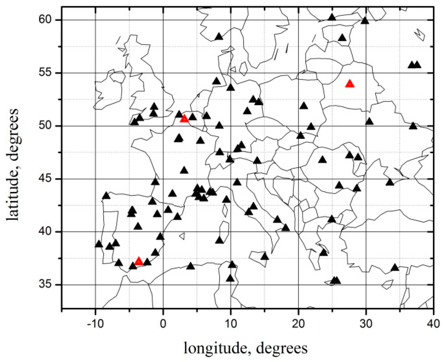
2.2. AERONET AOD Observations
2.3. Background Estimate
2.3.1. Climatology Data as a Background
2.3.2. Model Output as a Background
3. Results and Discussion
4. Conclusions
- The present study confirms the capability of STOI to fill spatial and temporal gaps in observations;
- The STOI estimates are sensitive to the choice of the background in areas with sparsely distributed observations;
- Using both the model output and climatology data as backgrounds allows for reducing the uncertainty in the estimate in areas where observations are limited in space and time without significantly increasing the computational cost.
Author Contributions
Funding
Institutional Review Board Statement
Informed Consent Statement
Data Availability Statement
Conflicts of Interest
Abbreviations
| AOD | Aerosol optical depth |
| OI | Optimal interpolation |
| STOI | Spatial–temporal optimal interpolation |
| KF | Kalman filtering |
| 3D-Var | Three-dimensional variational |
| 4D-Var | Four-dimensional variational |
| AERONET | Aerosol Robotic Network |
| RMSE | Root mean square error |
Appendix A

| AERONET Site | Longitude | Latitude |
|---|---|---|
| Lille | 3.142° E | 50.612° N |
| Barcelona | 2.112° E | 41.389° N |
| Venice | 12.508° E | 45.314° N |
| Xanthi | 24.919° E | 41.147° N |
| Ispra | 8.627° E | 45.803° N |
| Mainz | 8.3° E | 49.999° N |
| Helgoland | 7.887° E | 54.178° N |
| Palaiseau | 2.215° E | 48.712° N |
| Paris | 2.356° E | 48.847° N |
| Moldova | 28.816° E | 47.001° N |
| IMS-METU-ERDEMLI | 34.255° E | 36.565° N |
| Kyiv | 30.497° E | 50.364° N |
| Hamburg | 9.973° E | 53.568° N |
| Modena | 10.945° E | 44.632° N |
| Moscow_MSU_MO | 37.522° E | 55.707° N |
| Minsk | 27.601° E | 53.92° N |
| Rome_Tor_Vergata | 12.647° E | 41.84° N |
| Leipzig | 12.435° E | 51.353° N |
| Davos | 9.844° E | 46.813° N |
| Munich_University | 11.573° E | 48.148° N |
| Lecce_University | 18.111° E | 40.335° N |
| ATHENS-NOA | 23.718° E | 37.972° N |
| Belsk | 20.792° E | 51.837° N |
| Villefranche | 7.329° E | 43.684° N |
| Palencia | 4.516° W | 41.989° N |
| Carpentras | 5.058° E | 44.083° N |
| Toulon | 6.009° E | 43.136° N |
| Dunkerque | 2.368° E | 51.035° N |
| Evora | 7.911° W | 38.568° N |
| Laegeren | 8.364° E | 47.478° N |
| Cabo_da_Roca | 9.498° W | 38.782° N |
| Granada | 3.605° W | 37.164° N |
| Gustav_Dalen_Tower | 17.467° E | 58.594° N |
| OHP_OBSERVATOIRE | 5.71° E | 43.935° N |
| Chilbolton | 1.437° W | 51.144° N |
| Helsinki_Lighthouse | 24.926° E | 59.949° N |
| Sevastopol | 33.517° E | 44.616° N |
| Brussels | 4.35° E | 50.783° N |
| Zvenigorod | 36.775° E | 55.695° N |
| Porquerolles | 6.161° E | 43.001° N |
| Burjassot | 0.42° W | 39.507° N |
| Bucharest_Inoe | 26.028° E | 44.348° N |
| Autilla | 4.603° W | 41.997° N |
| Kanzelhohe_Obs | 13.901° E | 46.677° N |
| Ersa | 9.359° E | 43.004° N |
| Arcachon | 1.163° W | 44.664° N |
| Wytham_Woods | 1.332° W | 51.77° N |
| Malaga | 4.478° W | 36.715° N |
| Birkenes | 8.252° E | 58.388° N |
| Eforie | 28.632° E | 44.075° N |
| Huelva | 6.569° W | 37.016° N |
| Aubiere_LAMP | 3.111° E | 45.761° N |
| Frioul | 5.293° E | 43.266° N |
| CLUJ_UBB | 23.551° E | 46.768° N |
| Gloria | 29.36° E | 44.6° N |
| Bari_University | 16.884° E | 41.108° N |
| Tabernas_PSA-DLR | 2.358° W | 37.091° N |
| Calern_OCA | 6.923° E | 43.752° N |
| Montsec | 0.73° E | 42.051° N |
| Bure_OPE | 5.505° E | 48.562° N |
| Coruna | 8.421° W | 43.363° N |
| Madrid | 3.724° W | 40.452° N |
| Tizi_Ouzou | 4.056° E | 36.699° N |
| Iasi_LOASL | 27.556° E | 47.193° N |
| Zaragoza | 0.882° W | 41.633° N |
| FZJ-JOYCE | 6.413° E | 50.908° N |
| Badajoz | 7.011° W | 38.883° N |
| Cerro_Poyos | 3.487° W | 37.109° N |
| Valladolid | 4.706° W | 41.664° N |
| Murcia | 1.171° W | 38.001° N |
| MetObs_Lindenberg | 14.121° E | 52.209° N |
| Ben_Salem | 9.914° E | 35.551° N |
| CENER | 1.602° W | 42.816° N |
| HohenpeissenbergDWD | 11.012° E | 47.802° N |
| Galata_Platform | 28.193° E | 43.045° N |
| Tunis_Carthage | 10.2° E | 36.839° N |
| Carloforte | 8.31° E | 39.14° N |
| Exeter_MO | 3.475° W | 50.729° N |
| Strzyzow | 21.861° E | 49.879° N |
| LAQUILA_Coppito | 13.351° E | 42.368° N |
| Toulouse_MF | 1.374° E | 43.573° N |
| Martova | 36.953° E | 49.936° N |
| Zeebrugge-MOW1 | 3.12° E | 51.362° N |
| Peterhof | 29.826° E | 59.881° N |
| Finokalia-FKL | 25.67° E | 35.338° N |
| Berlin_FUB | 13.31° E | 52.458° N |
References
- Lahoz, W.A. Data Assimilation; Springer: Berlin/Heidelberg, Germany, 2010. [Google Scholar]
- Sandu, A.; Chai, T. Chemical Data Assimilation—An Overview. Atmosphere 2011, 2, 426–463. [Google Scholar] [CrossRef]
- Bocquet, M.; Elbern, H.; Eskes, H.; Hirtl, M.; Žabkar, R.; Carmichael, G.R.; Flemming, J.; Inness, A.; Pagowski, M.; Pérez Camaño, J.L.; et al. Data Assimilation in Atmospheric Chemistry Models: Current Status and Future Prospects for Coupled Chemistry Meteorology Models. Atmos. Chem. Phys. 2015, 15, 5325–5358. [Google Scholar] [CrossRef]
- Kalnay, E. Atmospheric Modeling, Data Assimilation and Predictability; Cambridge University Press: Cambridge, UK, 2002. [Google Scholar]
- Wikle, C.K.; Berliner, L.M. A Bayesian Tutorial for Data Assimilation. Phys. D Nonlinear Phenom. 2007, 230, 1–16. [Google Scholar] [CrossRef]
- Daley, R. Atmospheric Data Analysis; Cambridge University Press: Cambridge, UK, 1991. [Google Scholar]
- Rodgers, C.D. Inverse Methods for Atmospheric Sounding: Theory and Practice; World Scientific: Singapore, 2000. [Google Scholar]
- Gandin, L.S. Objective Analysis of Meteorological Fields; Gidrometeorol. Izd.: Leningrad, Russia, 1963. [Google Scholar]
- Lorenc, A.C. A Global Three-Dimensional Multivariate Statistical Analysis Scheme. Mon. Weather Rev. 1981, 109, 701–721. [Google Scholar] [CrossRef]
- Kalman, R.E. A New Approach to Linear Filtering and Prediction Problems. J. Basic Eng. 1960, 82, 35–45. [Google Scholar] [CrossRef]
- Constantinescu, E.M.; Sandu, A.; Chai, T.; Carmichael, G. Ensemble-based Chemical Data Assimilation: General Approach. Q. J. R. Meteorol. Soc. 2007, 133, 1229–1243. [Google Scholar] [CrossRef]
- Perrot, A.; Pannekoucke, O.; Guidard, V. Toward a Multivariate Formulation of the Parametric Kalman Filter Assimilation: Application to a Simplified Chemical Transport Model. Nonlin. Processes Geophys. 2023, 30, 139–166. [Google Scholar] [CrossRef]
- Sasaki, Y. An Objective Analysis Based on the Variational Method. J. Meteorol. Soc. Jpn. 1958, 36, 77–88. [Google Scholar] [CrossRef]
- Le Dimet, F.-X.; Talagrand, O. Variational Algorithms for Analysis and Assimilation of Meteorological Observations: Theoretical Aspects. Tellus 1986, 38A, 97–110. [Google Scholar] [CrossRef]
- Zang, Z.; You, W.; Ye, H.; Liang, Y.; Li, Y.; Wang, D.; Hu, Y.; Yan, P. 3DVAR Aerosol Data Assimilation and Evaluation Using Surface PM2.5, Himawari-8 AOD and CALIPSO Profile Observations in the North China. Remote Sens. 2022, 14, 4009. [Google Scholar] [CrossRef]
- Courtier, P.; Thepaut, J.-N.; Hollingsworth, A. A Strategy for Operational Implementation of 4D-Var, Using an Incremental Approach. Q. J. R. Meteorol. Soc. 1994, 120, 1367–1387. [Google Scholar] [CrossRef]
- Carmichael, G.R.; Sandu, A.; Chai, T.; Daescu, D.N.; Constantinescu, E.M.; Tang, Y. Predicting Air Quality: Improvements through Advanced Methods to Integrate Models and Measurements. J. Comput. Phys. 2008, 227, 3540–3571. [Google Scholar] [CrossRef]
- Tian, X.; Zhang, H.; Feng, X.; Li, X. i4DVar: An Integral Correcting Four-Dimensional Variational Data Assimilation Method. Earth Space Sci. 2021, 8, e2021EA001767. [Google Scholar] [CrossRef]
- Wahba, G.; Wendelberger, J. Some New Mathematical Methods for Variational Objective Analysis Using Splines and Cross Validation. Mon. Wea. Rev. 1980, 108, 1122–1143. [Google Scholar] [CrossRef]
- Lorenc, A.C. Analysis Methods for Numerical Weather Prediction. Q. J. R. Meteorol. Soc. 1986, 112, 1177–1194. [Google Scholar] [CrossRef]
- Candiani, G.; Carnevale, C.; Finzi, G.; Pisoni, E.; Volta, M. A Comparison of Reanalysis Techniques: Applying Optimal Interpolation and Ensemble Kalman Filtering to Improve Air Quality Monitoring at Mesoscale. Sci. Total Environ. 2013, 458–460, 7–14. [Google Scholar] [CrossRef]
- Zhao, M.; Dai, T.; Goto, D.; Wang, H.; Shi, G. Assessing the Assimilation of Himawari-8 Observations on Aerosol Forecasts and Radiative Effects during Pollution Transport from South Asia to the Tibetan Plateau. Atmos. Chem. Phys. 2024, 24, 235–258. [Google Scholar] [CrossRef]
- Fang, L.; Jin, J.; Segers, A.; Liao, H.; Li, K.; Xu, B.; Han, W.; Pang, M.; Lin, H.X. A Gridded Air Quality Forecast through Fusing Site-available Machine Learning Predictions from RFSML v1.0 and Chemical Transport Model Results from GEOS-Chem v13.1.0 using the Ensemble Kalman Filter. Geosci. Model Dev. 2023, 16, 4867–4882. [Google Scholar] [CrossRef]
- Jin, J.; Fang, L.; Li, B.; Liao, H.; Wang, Y.; Han, W.; Li, K.; Pang, M.; Wu, X.; Lin, H.X. 4DEnVar-based Inversion System for Ammonia Emission Estimation in China through Assimilating IASI Ammonia Retrievals. Environ. Res. Lett. 2023, 18, 034005. [Google Scholar] [CrossRef]
- Pouyaei, A.; Mizzi, A.P.; Choi, Y.; Mousavinezhad, S.; Khorshidian, N. Downwind Ozone Changes of the 2019 Williams Flats Wildfire: Insights from WRF-Chem/DART Assimilation of OMI NO2, HCHO, and MODIS AOD Retrievals. J. Geophys. Res. Atmos. 2023, 128, e2022JD038019. [Google Scholar] [CrossRef]
- Khattatov, B.V.; Gille, J.C.; Lyjak, L.V.; Brasseur, G.P.; Dvortsov, V.L.; Roche, A.E.; Waters, J. Assimilation of Photochemically Active Species and a Case Analysis of UARS Data. J. Geophys. Res. 1999, 104, 18715–18737. [Google Scholar] [CrossRef]
- Tombette, M.; Mallet, V.; Sportisse, B. PM10 Data Assimilation over Europe with the Optimal Interpolation Method. Atmos. Chem. Phys. 2009, 9, 57–70. [Google Scholar] [CrossRef]
- Miatselskaya, N.S.; Bril, A.I.; Chaikovsky, A.P.; Yukhymchuk, Y.Y.; Milinevski, G.P.; Simon, A.A. Optimal Interpolation of AERONET Radiometric Network Observations for the Evaluation of the Aerosol Optical Thickness Distribution in the Eastern European Region. J. Appl. Spectrosc. 2022, 89, 296–302. [Google Scholar] [CrossRef]
- Miatselskaya, N.; Milinevsky, G.; Bril, A.; Chaikovsky, A.; Miskevich, A.; Yukhymchuk, Y. Application of Optimal Interpolation to Spatially and Temporally Sparse Observations of Aerosol Optical Depth. Atmosphere 2023, 14, 32. [Google Scholar] [CrossRef]
- Donkelaar, A.; Martin, R.V.; Park, R.J. Estimating Ground-level PM2.5 with Aerosol Optical Depth Determined from Satellite Remote Sensing. J. Geophys. Res. 2006, 111, D21201. [Google Scholar] [CrossRef]
- Perez-Ramirez, D.; Veselovskii, I.; Whiteman, D.N.; Suvorina, A.; Korenskiy, M.; Kolgotin, A.; Holben, B.; Dubovik, O.; Siniuk, A.; Alados-Arboledas, L. High Temporal Resolution Estimates of Columnar Aerosol Microphysical Parameters from Spectrum of Aerosol Optical Depth by Linear Estimation: Application to Long-term AERONET and Star-photometry Measurements. Atmos. Meas. Tech. 2015, 8, 3117–3133. [Google Scholar] [CrossRef]
- Yu, H.; Dickinson, R.E.; Chin, M.; Kaufman, Y.J.; Geogdzhayev, B.; Mishchenko, M.I. Annual Cycle of Global Distributions of Aerosol Optical Depth from Integration of MODIS Retrievals and GOCART Model Simulations. J. Geophys. Res. 2003, 108, 4128. [Google Scholar] [CrossRef]
- Adhikary, B.; Kulkarni, S.; Dallura, A.; Tang, Y.; Chai, T.; Leung, L.R.; Qian, Y.; Chung, C.E.; Ramanathan, V.; Carmichael, G.R. A Regional Scale Chemical Transport Modeling of Asian Aerosols with Data Assimilation of AOD Observations Using Optimal Interpolation Technique. Atmos. Environ. 2008, 42, 8600–8615. [Google Scholar] [CrossRef]
- Rubin, J.I.; Reid, J.S.; Hansen, J.A.; Anderson, J.L.; Holben, B.N.; Xian, P.; Westphal, D.L.; Zhang, J. Assimilation of AERONET and MODIS AOT Observations Using Variational and Ensemble Data Assimilation Methods and Its Impact on Aerosol Forecasting Skill. J. Geophys. Res.–Atmos. 2017, 122, 4967–4992. [Google Scholar] [CrossRef]
- Li, J.; Kahn, R.A.; Wei, J.; Carlson, B.E.; Lacis, A.A.; Li, Z.; Li, X.; Dubovik, O.; Nakajima, T. Synergy of Satellite- and Ground-based Aerosol Optical Depth Measurements using an Ensemble Kalman Filter Approach. J. Geophys. Res. Atmos. 2020, 125, e2019JD031884. [Google Scholar] [CrossRef]
- Huang, B.; Pagowski, M.; Trahan, S.; Martin, C.R.; Tangborn, A.; Kondragunta, S.; Kleist, D.T. JEDI-based Three-Dimensional Ensemble-Variational Data Assimilation System for Global Aerosol Forecasting at NCEP. J. Adv. Model. Earth Syst. 2023, 15, e2022MS003232. [Google Scholar] [CrossRef]
- Goto, D.; Nishizawa, T.; Uchida, J.; Yumimoto, K.; Jin, Y.; Higurashi, A.; Shimizu, A.; Sugata, S.; Yashiro, H.; Hayasaki, M.; et al. Development of an Aerosol Assimilation System Using a Global Non-Hydrostatic Model, a 2-Dimensional Variational Method, and Multiple Satellite-Based Aerosol Products. J. Adv. Model. Earth Syst. 2024, 16, e2023MS004046. [Google Scholar] [CrossRef]
- Collins, W.D.; Rasch, P.J.; Eaton, B.E.; Khattatov, B.V.; Lamarque, J.-F.; Zender, C.S. Simulating Aerosols Using a Chemical Transport Model with Assimilation of Satellite Aerosol Retrievals: Methodology for INDOEX. J. Geophys. Res. Atmos. 2001, 106, 7313–7336. [Google Scholar] [CrossRef]
- Xue, Y.; Xu, H.; Guang, J.; Mei, L.; Guo, J.; Li, C.; Mikusauskas, R.; He, X. Observation of an Agricultural Biomass Burning in Central and East China Using Merged Aerosol Optical Depth Data from Multiple Satellite Missions. Int. J. Remote Sens. 2014, 35, 5971–5983. [Google Scholar] [CrossRef]
- Li, K.; Bai, K.; Li, Z.; Guo, J.; Chang, N.-B. Synergistic Data Fusion of Multimodal AOD and Air Quality Data for Near Real-Time Full Coverage Air Pollution Assessment. J. Environ. Manag. 2022, 302, 114121. [Google Scholar] [CrossRef]
- Holben, B.N.; Eck, T.F.; Slutsker, I.; Tanre, D.; Buis, J.P.; Setzer, A.; Vermote, E.; Reagan, J.A.; Kaufman, Y.J.; Nakajima, T.; et al. AERONET—A Federated Instrument Network and Data Archive for Aerosol Characterization. Remote Sens. Environ. 1998, 66, 1–16. [Google Scholar] [CrossRef]
- Holben, B.N.; Kim, J.; Sano, I.; Mukai, S.; Eck, T.F.; Giles, D.M.; Schafer, J.S.; Sinyuk, A.; Slutsker, I.; Smirnov, A. An Overview of Mesoscale Aerosol Processes, Comparisons, and Validation Studies from DRAGON Networks. Atmos. Chem. Phys. 2018, 18, 655–671. [Google Scholar] [CrossRef]
- Giles, D.M.; Sinyuk, A.; Sorokin, M.G.; Schafer, J.S.; Smirnov, A.; Slutsker, I.; Eck, T.F.; Holben, B.N.; Lewis, J.R.; Campbell, J.R.; et al. Advancements in the Aerosol Robotic Network (AERONET) Version 3 Database—Automated Near-Real-Time Quality Control Algorithm with Improved Cloud Screening for Sun Photometer Aerosol Optical Depth (AOD) Measurements. Atmos. Meas. Tech. 2019, 12, 169–209. [Google Scholar] [CrossRef]
- Cimel Electronique. Available online: https://www.cimel.fr/ (accessed on 10 April 2025).
- Dubovik, O.; King, M.D. A Flexible Inversion Algorithm for Retrieval of Aerosol Optical Properties from Sun and Sky Radiance Measurements. J. Geophys. Res. 2000, 105, 20673–20696. [Google Scholar] [CrossRef]
- NASA, Goddard Spase Flight Center; AERONET; Aerosol Robotic Network. Available online: https://aeronet.gsfc.nasa.gov/ (accessed on 16 April 2025).
- Eck, T.F.; Holben, B.N.; Reid, J.S.; Dubovik, O.; Smirnov, A.; O’Neill, N.T.; Slutsker, I.; Kinne, S. Wavelength Dependence of the Optical Depth of Biomass Burning, Urban and Desert Dust Aerosols. J. Geophys. Res. 1999, 104, 31333–31349. [Google Scholar] [CrossRef]
- Holben, B.N.; Tanre, D.; Smirnov, A.; Eck, T.F.; Slutsker, I.; Abuhassan, N.; Newcomb, W.W.; Schafer, J.; Chatenet, B.; Lavenue, F.; et al. An Emerging Ground-Based Aerosol Climatology: Aerosol Optical Depth from AERONET. J. Geophys. Res. 2001, 106, 12067–12097. [Google Scholar] [CrossRef]
- GEOS-Chem. Available online: https://geoschem.github.io (accessed on 10 April 2025).
- Bey, I.; Jacob, D.J.; Yantosca, R.M.; Logan, J.A.; Field, B.D.; Fiore, A.M.; Li, Q.; Liu, H.Y.; Mickley, L.J.; Schultz, M.G. Global Modeling of Tropospheric Chemistry with Assimilated Meteorology: Model Description and Evaluation. J. Geophys. Res. 2001, 106, 23073–23096. [Google Scholar] [CrossRef]
- Park, R.J.; Jacob, D.J.; Field, B.D.; Yantosca, R.M.; Chin, M. Natural and Transboundary Pollution Influences on Sulfate-Nitrate-Ammonium Aerosols in the United States: Implications for Policy. J. Geophys. Res. 2004, 109, D15204. [Google Scholar] [CrossRef]
- NASA, Goddard Space Flight Center; Global Modeling and Assimilation Office; GEOS Systems. Available online: https://gmao.gsfc.nasa.gov/GEOS_systems/ (accessed on 16 April 2025).
- Keller, C.A.; Long, M.S.; Yantosca, R.M.; Da Silva, A.M.; Pawson, S.; Jacob, D.J. HEMCO v1.0: A Versatile, ESMF-Compliant Component for Calculating Emissions in Atmospheric Models. Geosci. Model Dev. 2014, 7, 1409–1417. [Google Scholar] [CrossRef]
- Lin, S.-J.; Rood, R.B. Multidimensional Flux Form Semi-Lagrangian Transport Schemes. Mon. Weather Rev. 1996, 124, 2046–2070. [Google Scholar] [CrossRef]
- Sherwen, T.; Schmidt, J.A.; Evans, M.J.; Carpenter, L.J.; Grossmann, K.; Eastham, S.D.; Jacob, D.J.; Dix, B.; Koenig, T.K.; Sinreich, R.; et al. Global Impacts of Tropospheric Halogens (Cl, Br, I) on Oxidants and Composition in GEOS-Chem. Atmos. Chem. Phys. 2016, 16, 12239–12271. [Google Scholar] [CrossRef]
- Travis, K.R.; Jacob, D.J.; Fisher, J.A.; Kim, P.S.; Marais, E.A.; Zhu, L.; Yu, K.; Miller, C.C.; Yantosca, R.M.; Sulprizio, M.P.; et al. Why Do Models Overestimate Surface Ozone in the Southeast United States? Atmos. Chem. Phys. 2016, 16, 13561–13577. [Google Scholar] [CrossRef]
- Eastham, S.D.; Weisenstein, D.K.; Barrett, S.R.H. Development and Evaluation of the Unified Tropospheric–Stratospheric Chemistry Extension (UCX) for the Global Chemistry-Transport Model GEOS-Chem. Atmos. Environ. 2014, 89, 52–63. [Google Scholar] [CrossRef]
- Latimer, R.N.C.; Martin, R.V. Interpretation of Measured Aerosol Mass Scattering Efficiency over North America Using a Chemical Transport Model. Atmos. Chem. Phys. 2019, 19, 2635–2653. [Google Scholar] [CrossRef]
- Ridley, D.A.; Heald, C.L.; Ford, B. North African Dust Export and Deposition: A Satellite and Model Perspective. J. Geophys. Res. 2012, 117, D02202. [Google Scholar] [CrossRef]
- Wang, Y.X.; Mcelroy, M.B.; Jacob, D.J.; Yantosca, R.M. A Nested Grid Formulation for Chemical Transport over Asia: Applications to CO. J. Geophys. Res. Atmos. 2004, 109, D22307. [Google Scholar] [CrossRef]
- Zhang, L.; Liu, L.; Zhao, Y.; Gong, S.; Zhang, Z.; Henze, D.K.; Capps, S.L.; Fu, T.-M.; Zhang, Q.; Wang, Y. Source Attribution of Particulate Matter Pollution over North China with the Adjoint Method. Environ. Res. Lett. 2015, 10, 084011. [Google Scholar] [CrossRef]
- Kim, P.S.; Jacob, D.J.; Fisher, J.A.; Travis, K.; Yu, K.; Zhu, L.; Yantosca, R.M.; Sulprizio, M.P.; Jimenez, J.L.; Campuzano-Jost, P.; et al. Sources, Seasonality, and Trends of Southeast US Aerosol: An Integrated Analysis of Surface, Aircraft, and Satellite Observations with the GEOS-Chem Model. Atmos. Chem. Phys. 2015, 15, 10411–10433. [Google Scholar] [CrossRef]
- Li, S.; Garay, M.J.; Chen, L.; Rees, E.; Liu, Y. Comparison of GEOS-Chem Aerosol Optical Depth with AERONET and MISR Data over the Contiguous United States. J. Geophys. Res. 2013, 118, 11228–11241. [Google Scholar] [CrossRef]
- Curci, G.; Hogrefe, C.; Bianconi, R.; Im, U.; Balzarini, A.; Baró, R.; Brunner, D.; Forkel, R.; Giordano, L.; Hirtl, M.; et al. Uncertainties of Simulated Aerosol Optical Properties Induced by Assumptions on Aerosol Physical and Chemical Properties: An AQMEII-2 Perspective. Atmos. Environ. 2015, 115, 541–552. [Google Scholar] [CrossRef]
| Wavelength nm | Granada | Lille | Minsk | |||
|---|---|---|---|---|---|---|
| GEOS-Chem | STOI | GEOS-Chem | STOI | GEOS-Chem | STOI | |
| 440 | 0.142 | 0.064 (55%) | 0.116 | 0.094 (19%) | 0.130 | 0.103 (21%) |
| 675 | 0.128 | 0.048 (62%) | 0.089 | 0.077 (14%) | 0.074 | 0.070 (7%) |
| 870 | 0.125 | 0.046 (63%) | 0.081 | 0.070 (13%) | 0.055 | 0.059 (−7%) |
| Wavelength nm | Granada | Lille | Minsk | |||
|---|---|---|---|---|---|---|
| GEOS-Chem | STOI | GEOS-Chem | STOI | GEOS-Chem | STOI | |
| 440 | 0.142 | 0.064 (55%) | 0.116 | 0.101 (13%) | 0.130 | 0.128 (1%) |
| 675 | 0.128 | 0.048 (63%) | 0.089 | 0.079 (10%) | 0.074 | 0.069 (8%) |
| 870 | 0.125 | 0.045 (64%) | 0.081 | 0.071 (12%) | 0.055 | 0.047 (14%) |
| Wavelength nm | Granada | Lille | Minsk | |||
|---|---|---|---|---|---|---|
| GEOS-Chem | STOI | GEOS-Chem | STOI | GEOS-Chem | STOI | |
| 440 | 0.142 | 0.063 (56%) | 0.116 | 0.095 (18%) | 0.130 | 0.103 (20%) |
| 675 | 0.128 | 0.047 (63%) | 0.089 | 0.077 (14%) | 0.074 | 0.060 (20%) |
| 870 | 0.125 | 0.045 (64%) | 0.081 | 0.070 (13%) | 0.055 | 0.044 (19%) |
Disclaimer/Publisher’s Note: The statements, opinions and data contained in all publications are solely those of the individual author(s) and contributor(s) and not of MDPI and/or the editor(s). MDPI and/or the editor(s) disclaim responsibility for any injury to people or property resulting from any ideas, methods, instructions or products referred to in the content. |
© 2025 by the authors. Licensee MDPI, Basel, Switzerland. This article is an open access article distributed under the terms and conditions of the Creative Commons Attribution (CC BY) license (https://creativecommons.org/licenses/by/4.0/).
Share and Cite
Miatselskaya, N.; Bril, A.; Chaikovsky, A. Using Chemical Transport Model and Climatology Data as Backgrounds for Aerosol Optical Depth Spatial–Temporal Optimal Interpolation. Atmosphere 2025, 16, 623. https://doi.org/10.3390/atmos16050623
Miatselskaya N, Bril A, Chaikovsky A. Using Chemical Transport Model and Climatology Data as Backgrounds for Aerosol Optical Depth Spatial–Temporal Optimal Interpolation. Atmosphere. 2025; 16(5):623. https://doi.org/10.3390/atmos16050623
Chicago/Turabian StyleMiatselskaya, Natallia, Andrey Bril, and Anatoly Chaikovsky. 2025. "Using Chemical Transport Model and Climatology Data as Backgrounds for Aerosol Optical Depth Spatial–Temporal Optimal Interpolation" Atmosphere 16, no. 5: 623. https://doi.org/10.3390/atmos16050623
APA StyleMiatselskaya, N., Bril, A., & Chaikovsky, A. (2025). Using Chemical Transport Model and Climatology Data as Backgrounds for Aerosol Optical Depth Spatial–Temporal Optimal Interpolation. Atmosphere, 16(5), 623. https://doi.org/10.3390/atmos16050623