Analysis of Time-Domain Characteristics of Microsecond-Scale Repetitive Pulse Discharge Events in Lightning

Abstract

To clarify the background of multiple burst (MB) specifications in the aviation lightning test standards, a broadband lightning electromagnetic field measurement system was employed to collect 91 sets of VLF/LF band nature flash data. A total of 719 typical repetitive pulse (RP) groups were identified, and 163,589 single pulse samples were analyzed statistically. The variational mode decomposition (VMD) method and a trend-free correlation on index (TFCI) were used to extract RPs from the slowly varying trends and high-frequency noises from the measured data. The time-domain characteristics of four kinds of RPs corresponding to the lightning discharge events—initial breakdown pulse (IBP), regular pulse bursts (RPB), chaotic pulse train (CPT), and dart-stepped leader (DSL)—were investigated. By comparing previous statistics and the definition in current international aviation standards, the intrinsic correlation between RPs and the defined parameters of MBs was explored. New recommendations for the MB test standard were subsequently proposed.

1. Introduction

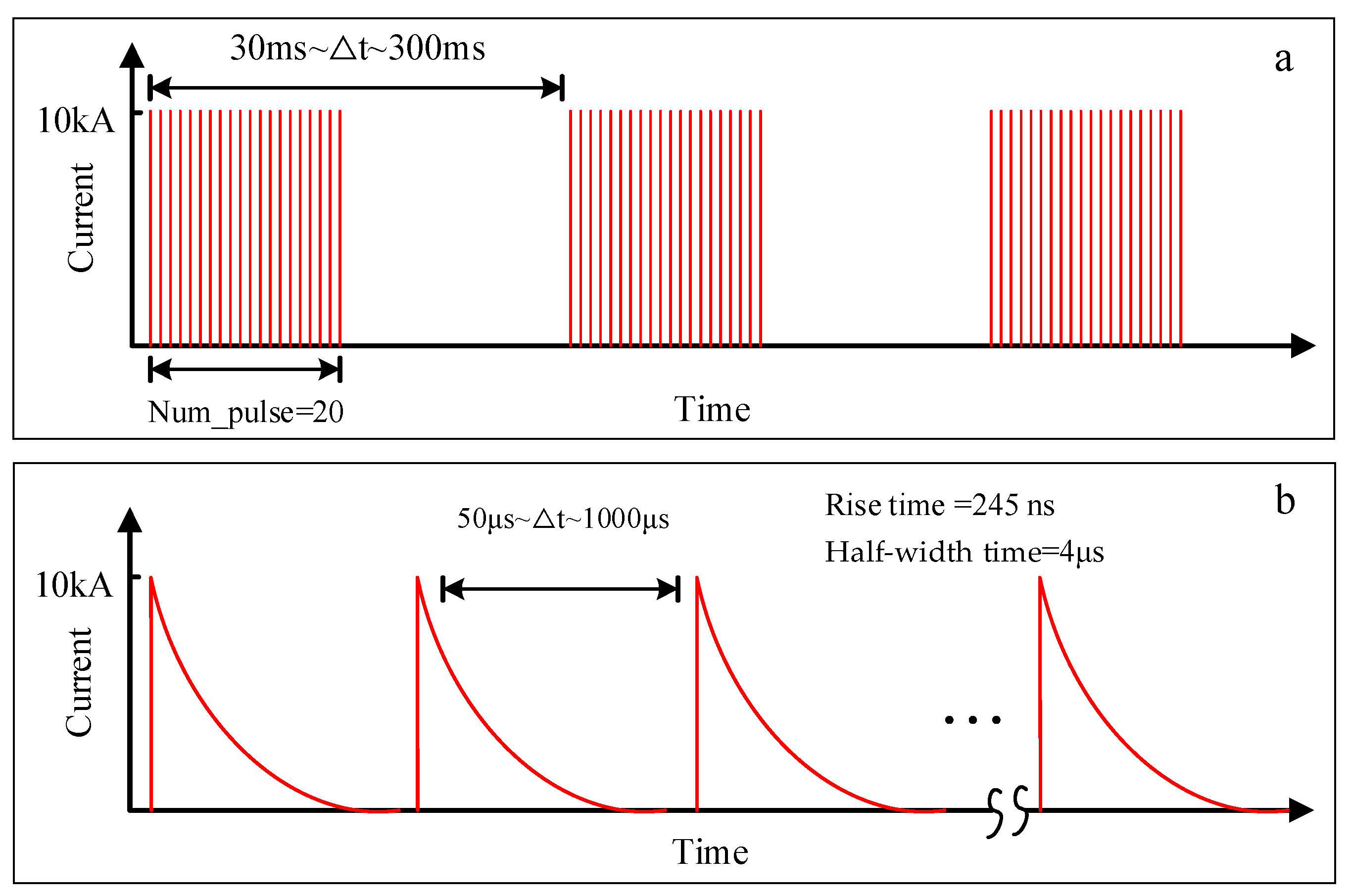
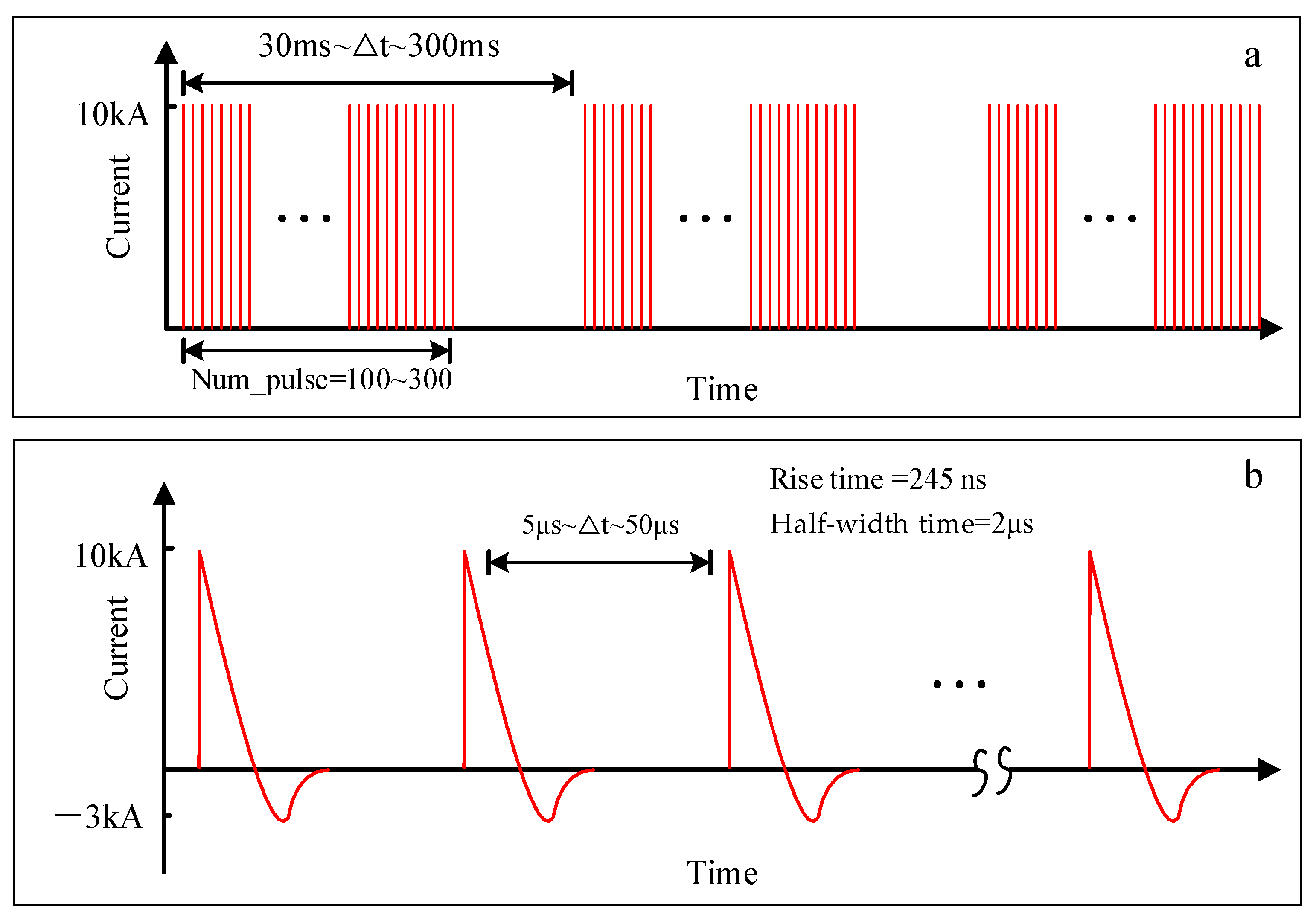
Natural lightning frequently demonstrates repetitive pulse (RP) discharge phenomena on the microsecond time scale during its occurrence and development. In the lightning test standards of SAE ARP 5412C [1] and section 22 in RTCA DO-160G [2], the test specifications of multiple burst (MB) waveform were set as three bursts of current pulses characterized by random time intervals of 30 to 300 ms, which are comprised of Component H waveforms with a leading edge time of 0.245 μs and a half-width time of 4 μs, and the time interval of individual pulses is 50 to 1000 μs, as illustrated in Figure 1.

In the lightning test environment, Components A, B, C, and D are employed to characterize the effects of the first return stroke, intermediate process, continuous current, and subsequent return strokes of lightning on aircraft. Specifically, Component A corresponds to the first return stroke with the highest current peak, featuring a pulse waveform duration of up to 500 μs, a rise time of 2.85 μs, and a current peak of 200 kA.

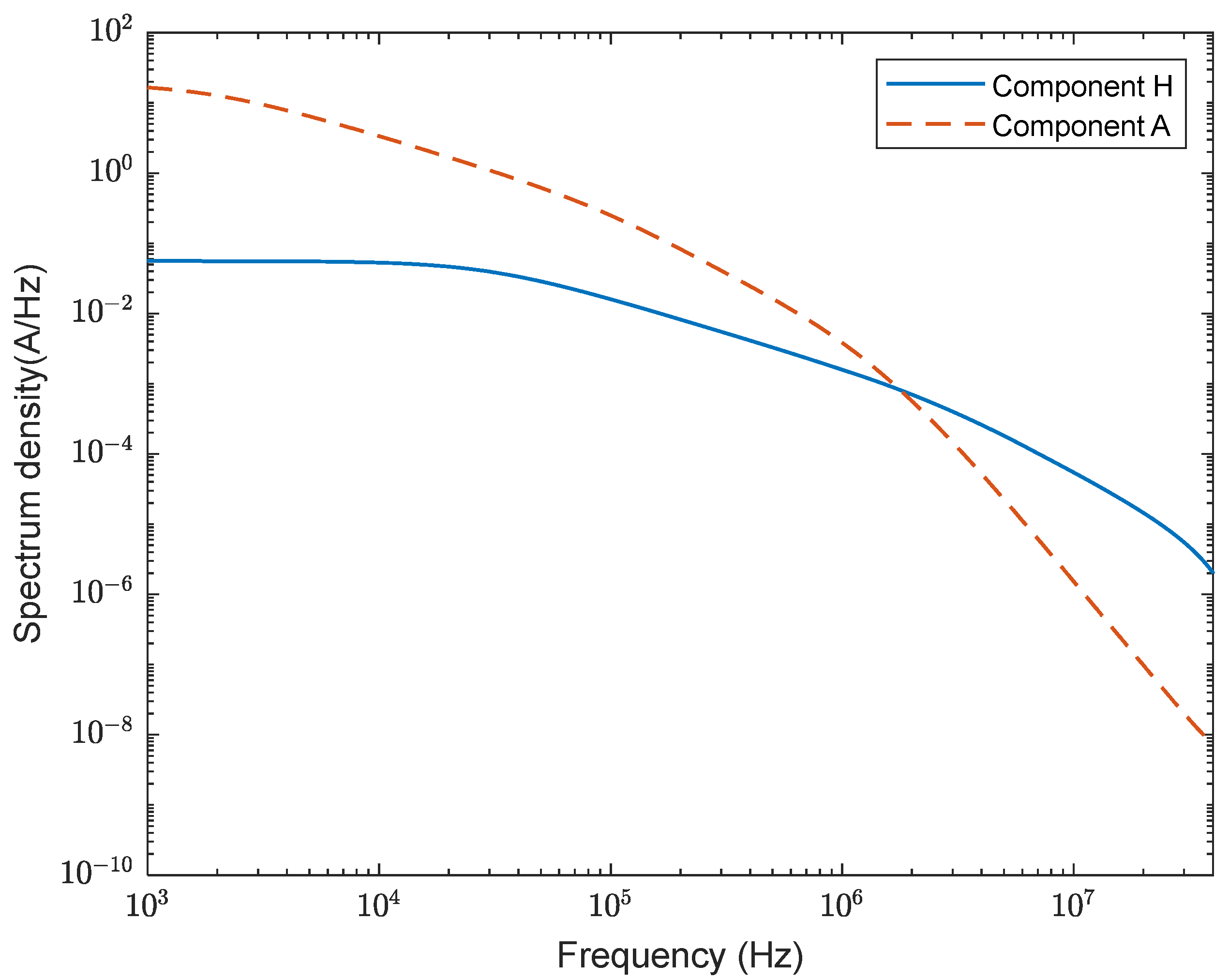
Although the peak current of a single Component H waveform is only 10 kA, its rise time is one order of magnitude faster than that of the Component A waveform, which is commonly employed in lightning tests. Consequently, the Component H waveform contains significantly richer high-frequency components. The spectral comparison between the Component H and A waveforms is illustrated in Figure 2. Therefore, the MB test environment differs substantially from the large-current, high-energy, single-pulse discharge processes characterized by the A, B, C, and D components in the lightning test environment.

There are currently two key issues in the research on lightning RP discharge events. First, the definition of the MB test environment in the current standards is based on SAE ARP, published in 1990. Due to the limitations of lightning observation data at that time, this definition may not fully align with the actual characteristics of repetitive pulse discharge events. Moreover, the source of this definition lacks a detailed explanation, and the physical process that the MB test environment represents in lightning remain unclear. Rakov et al. discussed the bursts of pulses in lightning magnetic radiation with their concern on observations and implications for lightning test standards in 1996 [3]. As stated by them, the observed regular pulse bursts (RPB) exhibit some similarity to Component H, but neither the present definition of the H component nor its newly proposed revision appears to be based on adequate experimental data.

In recent decades, the microsecond-scale repetitive pulse discharge events have been investigated by many research groups from the viewpoint of lightning physics. These studies primarily focus on phenomena such as initial breakdown pulse (IBP), regular pulse burst (RPB), chaotic pulse train (CPT), and dart-stepped leader (DSL) [4].

Based on lightning electromagnetic field observation data, Krider et al. investigated the time-domain parameter characteristics of intra-cloud RPBs and hypothesized that these pulse sequences are likely to occur at the moment of K changes. The time-domain waveform of these sequences was found to resemble that of dart-stepped leaders. They attributed RPBs to the “intracloud dart-stepped leader process”, with each RPB lasting between 100 and 400 μs and manifesting as a uniformly spaced pulse sequence (half-width time approximately 1 μs, pulse interval approximately 6.1 μs) [5]. Rakov et al. conducted an in-depth analysis of RPB data from six intracloud and cloud-to-ground flashes. They discovered that each RPB contained roughly several dozen pulses, with pulse widths of several microseconds and average pulse intervals ranging from 6 to 7 μs [3]. Wang Yanhui et al. utilized a VHF and VLF/LF dual-frequency lightning detection system to perform high-time-resolution analysis of RPB in lightning discharges over China’s inland plateau region. By statistically analyzing lightning data collected over a 15 min period, they compared and analyzed RPB parameters and lightning locations. Their results indicated that 83% of lightning events exhibited RPB, with pulse widths of approximately 1 μs, pulse intervals of approximately 5 μs, and durations ranging from 20 to 2000 μs, longer than those observed by Krider and Rakov et al. [6,7]. Kolmasova et al. examined regular unipolar microsecond-scale magnetic field pulse sequences generated by lightning discharges under continental conditions in Prague, Czech Republic. The observed sequences consisted of several dozen pulses, with pulse intervals ranging from 1 to 10 μs [8].

Chaotic Pulse Train (CPT) was first identified by Weidman in 1982 and initially referred to as Chaotic Leader (CL) [9]. Mäkelä et al. conducted direct measurements of the 10 MHz narrowband high-frequency radiation emitted by CL, revealing an average duration of approximately 300 μs. Gomes was the first to generalize the concept of CL to CPT, based on the observation that while most chaotic pulse activities occur prior to subsequent return strokes, similar phenomena have also been detected in some intense intracloud flashes. This suggests that CL is not necessarily associated with return strokes. Using a high-time-resolution observation system, it was found that the pulse width can be as short as 0.4 μs, with typical pulse intervals ranging from 2 to 20 μs and pulse durations spanning 400 to 500 μs [10,11]. Lan Yu et al. employed a broadband lightning observation system to perform time-frequency analysis of CPT. In the time domain, the average duration of CPT was determined to be 472 μs, with a range of 95 to 1445 μs (consistent with Gomes’ findings), and individual pulse widths were measured between 60 ns and 4 μs [12]. Some research teams have also employed time-domain analysis, frequency-domain analysis, wavelet analysis, high-speed cameras, VHF interferometers, X-ray radiation analysis, etc., to conduct observations and analyses of microsecond-scale RP discharge events [13,14,15,16,17,18,19,20,21].

Dart-stepped leader (DSL), which occurs subsequent to the initial lightning return stroke, exhibits a more optimized discharge channel compared with the stepped leader (SL). Consequently, it demonstrates a higher pulse repetition frequency and imposes stricter requirements on the standard testing environment for lightning protection systems. In this paper, DSL is selected as the primary subject of analysis. According to Rakov et al. [3], the pulse width of DSL typically ranges from 1 to 2 μs, with a pulse interval of 6 to 8 μs. Furthermore, Qie et al. [22] reported that the duration of the DSL pulse train is approximately 7.7 ms, the pulse interval is around 12.2 μs, and the pulse half-width is about 0.5 μs.

The initial breakdown pulses (IBPs) are a series of microsecond-scale repetitive pulse sequences that frequently occur during the initiation stage of lightning. Since this process occurs within the cloud and is obscured by the cloud body, its observation primarily depends on the measurement and inversion of ground electric field changes, as well as the localization of VHF electromagnetic radiation generated during the lightning breakdown process [23]. In 2023, Wu et al. analyzed the pulse rate and pulse width of the IBP train in lightning flashes in the Osaka area of Japan and emphasized the decreasing trends with increasing initiation altitude and increasing trends with increasing vertical speed. They also pointed out that the average pulse width of an IBP was 15.3 μs [24]. Several research teams have conducted analyses on the time-domain characteristics of the IBP pulse sequence [18,24,25,26,27,28,29,30,31,32]. For example, Qie et al. [28] reported that the duration of the IBP was 2.97 ms, with a full width of a single pulse at 21.11 μs. Additionally, Yoshida et al. [30] pointed out that the duration of the IBP was 2.7 ms and the interval of the IBP was 73 μs. Karunarathne et al. [31] indicated that the full width of the pulse was 25.2 μs and the rise time of the pulse was 12 μs. Cao, D.J. et al. [33] categorized IBPs into four classes based on normalized pulse amplitude: large pulses, medium pulses, small pulses, and extremely small pulses. Furthermore, according to pulse width, these pulses were classified into two groups: narrow pulses (≤10 μs) and wide pulses (>10 μs). Notably, small pulses with widths less than 10 μs are associated with breakdown discharges occurring at smaller spatial scales.

The primary aim of the aforementioned research is to elucidate the physical mechanisms underlying RP events and the relationships among them; almost none of them discussed their relationship with Component H in lightning test standards, except for [3]. In this paper, we report the measurement results of RP events in eastern China; time-domain features of four kinds of RPs are compared based on 719 sets of pulse trains. The variational mode decomposition (VMD) algorithm is employed to identify RPs from the measured waveform. The intrinsic correlation between RPs and the defined parameters of Component H is discussed. Based on these findings, new recommendations for the MB test standard were subsequently proposed.

2. Measurement System and Data

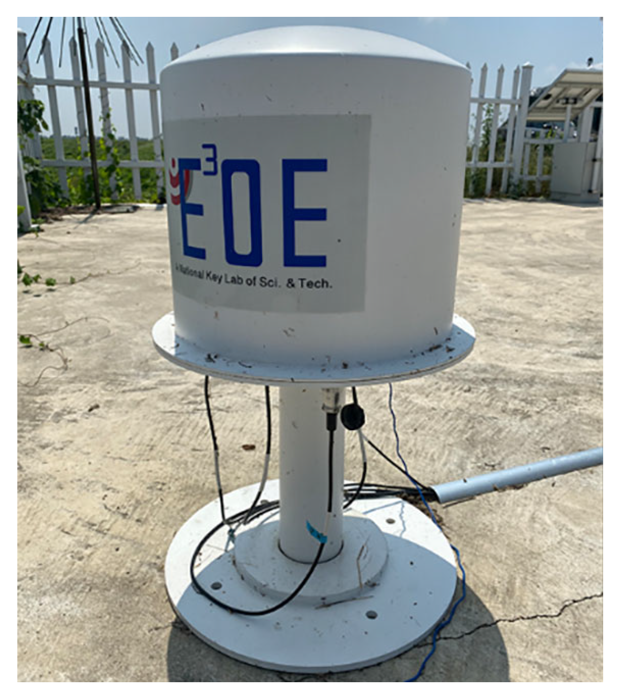
In this paper, our Jiangsu lightning observation team (SLOT) conducted lightning observation experiments utilizing a broadband lightning electromagnetic field measurement system, as depicted in Figure 3, which comprises fast and slow antennas for detecting rapid and gradual variations in the lightning electric field. The system is capable of simultaneously capturing both the rapidly changing component of the lightning electric field and the slowly varying component rich in electrostatic field contributions. This capability allows for a comprehensive representation of the superimposed relationship between microsecond-scale discharge events and slower millisecond-scale discharge events. Such an analysis plays a crucial role in identifying the physical characteristics of lightning phenomena.

The data samples analyzed in this paper consist of VLF/LF signals acquired by the fast antenna, which exhibits a sensitivity of 26 V/m/V and operates at a sampling frequency of 10 MHz [34].

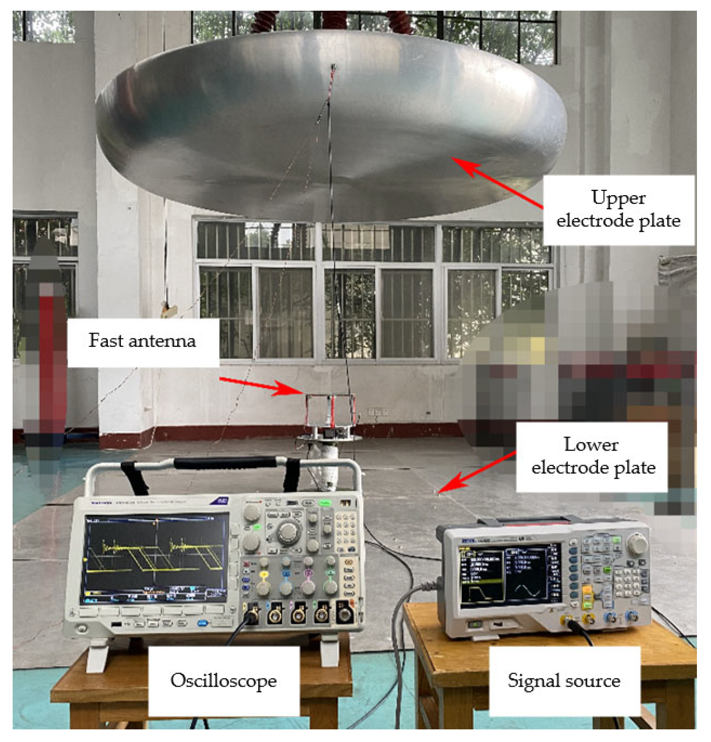
Figure 4 presents the schematic diagram of the laboratory calibration process for the fast antenna. In this setup, the metal disc serves as the upper electrode plate, while the grounded metal plate acts as the lower electrode plate. The upper electrode plate is connected to the output port of the signal source via a coaxial cable, and the lower electrode plate is electrically grounded. The fast antenna is positioned at the center of the metal floor, and the oscilloscope is employed to measure the output signal from the fast antenna. Specifically, the signal source is a Rigol DG4162 function/arbitrary waveform generator with an internal impedance of 50 Ω, capable of producing stable and continuous waveforms. The oscilloscope is a Tek 3024 model, featuring a bandwidth of 200 MHz and a maximum sampling rate of 2.5 GHz.

Assuming the voltage between the two plates is V and the distance between them is h, the electric field intensity between the plates can be determined as follows:

$$E={\displaystyle \frac{V}{h}}$$

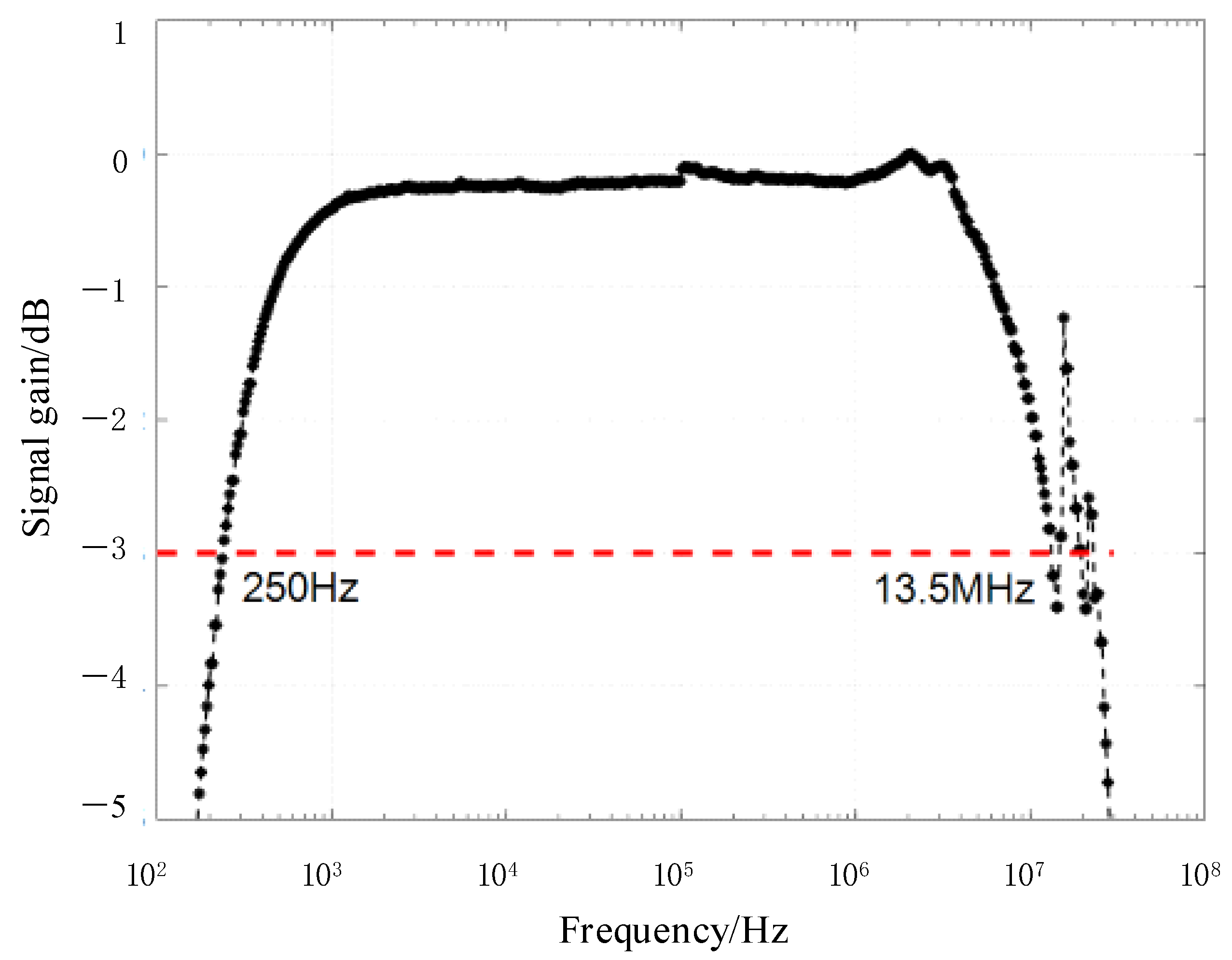
Sinusoidal waves with a voltage of 20 V and varying frequencies, generated by the signal source, are injected into the upper electrode. The output amplitude of the fast antenna varies as a function of frequency. The results of the continuous sinusoidal wave calibration for the fast antenna’s amplitude–frequency characteristic curve are presented in Figure 5. It can be observed that the fast antenna’s −3 dB bandwidth ranges from 250 Hz to 13.5 MHz, which is sufficient to satisfy the observational requirements for lightning signals at the sub-microsecond time scale.

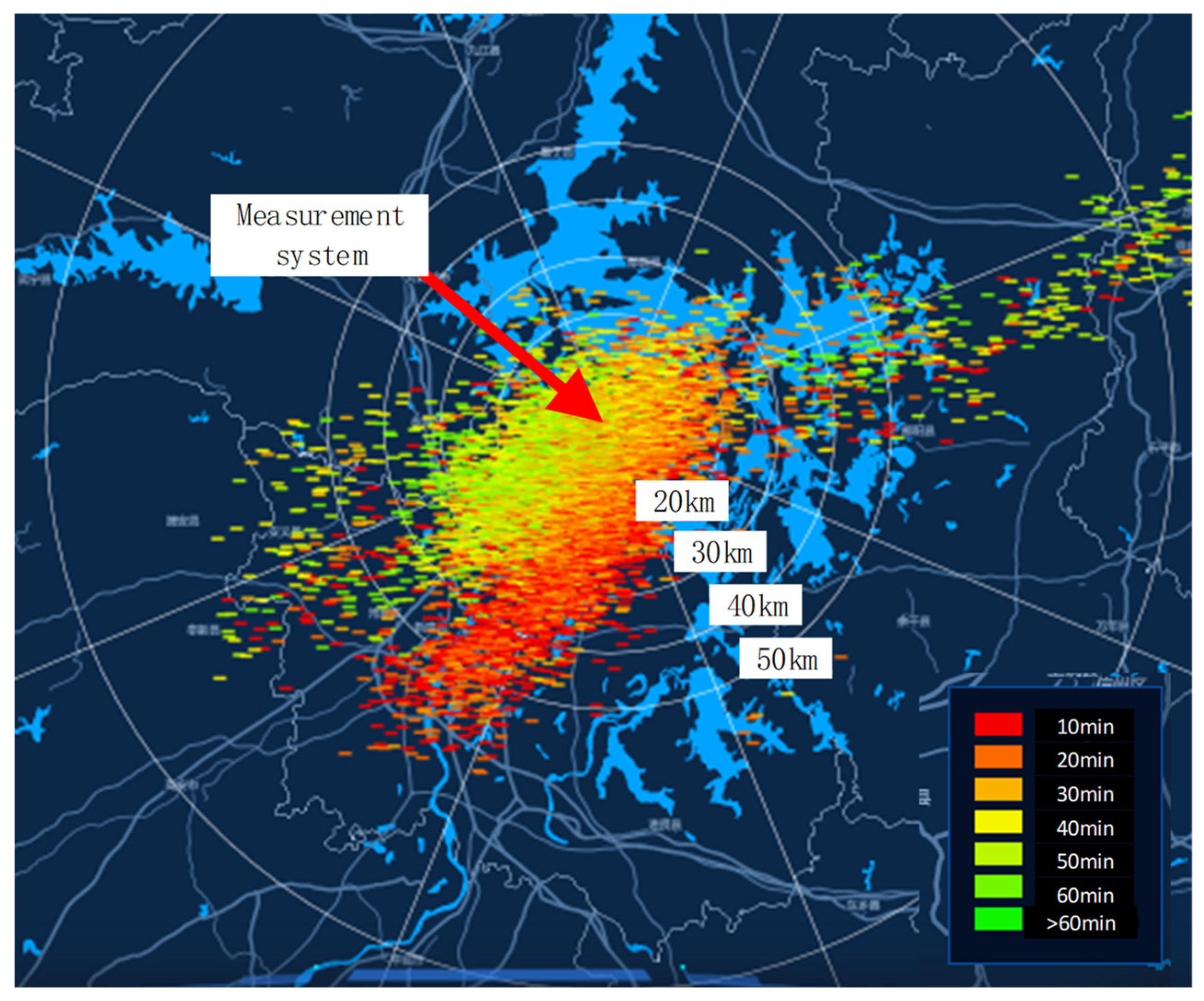
The samples analyzed in this paper were obtained from the lightning electric field data collected by our SLOT team in Jiangxi Province, China, between 10:00 and 11:00 on 29 June 2022. As shown in Figure 6, which displays the lightning location results during this period, most of the lightning events occurred within a 50 km radius of the measurement system. From these data, we extracted 91 relatively clear lightning waveforms for further analysis, and 1554 repetitive pulse sequences were identified. Among these, 719 relatively clear typical pulse sequence samples, including 46 IBP pulse sequences, 248 DSL pulse sequences, 353 RBP pulse sequences, and 72 CPT pulse sequences, were identified and extracted for classification and statistical analysis.

3. Time-Domain Feature Analysis Methodology

3.1. Identification Procedure for Repetitive Pulse Sequences

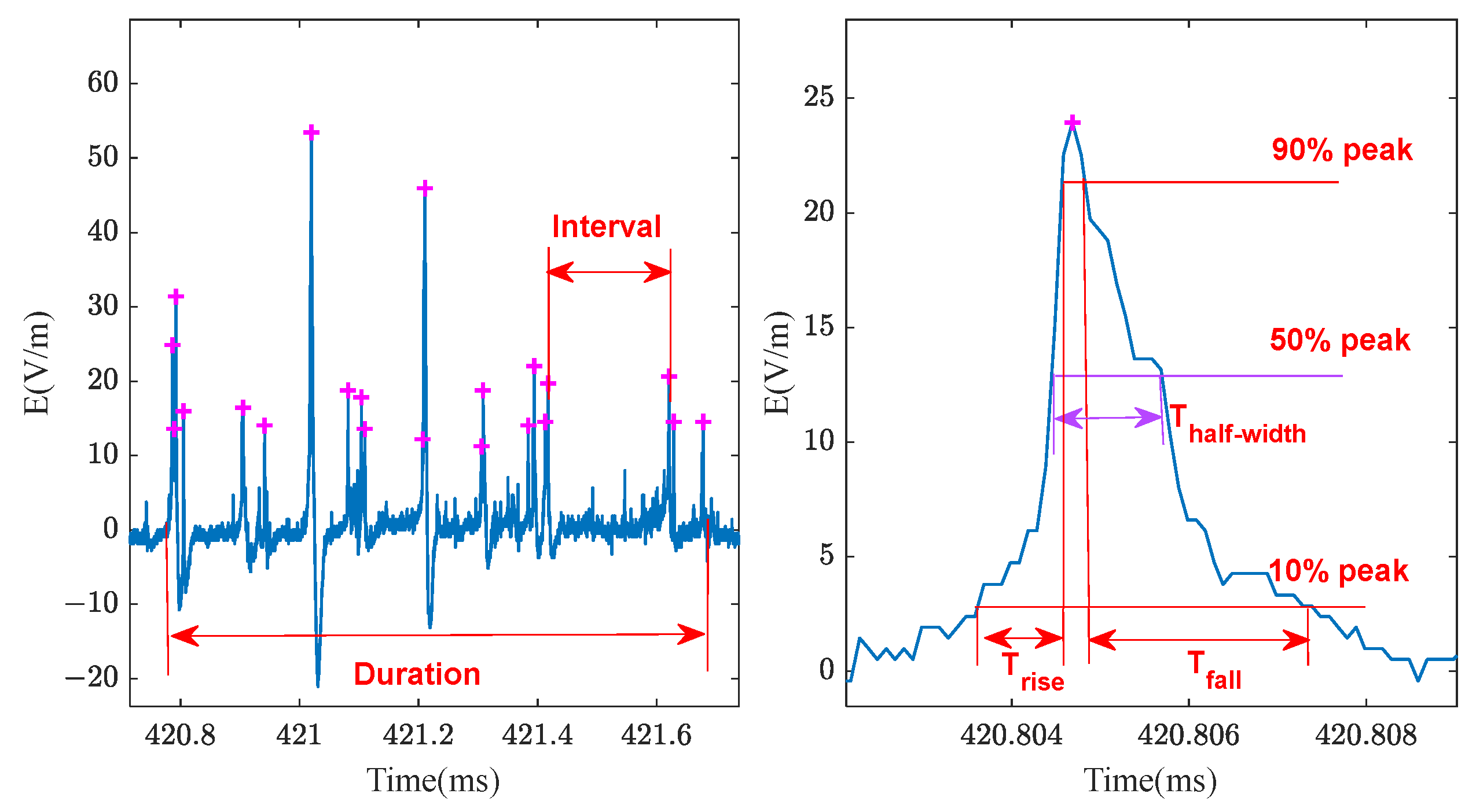
For the collected signal waveforms, time-domain characteristic parameters of repetitive pulse discharge events were extracted. These parameters primarily include the number of pulses in a pulse sequence, the duration of a pulse sequence, the minimum pulse interval, the average pulse interval, the average half-width and full-width of the pulse, the pulse rise time, and the pulse fall time, as depicted in Figure 7 in which the plus sign indicates the location of the extracted pulse peak point. Specifically, the rise time is defined as the time difference between 10% and 90% of the peak value of the rising edge, characterizing the high-frequency components of the signal. The fall time is defined as the time difference between 90% and 10% of the peak value of the falling edge, characterizing the low-frequency components of the signal. The half-width time refers to the time width of the pulse between two adjacent half-peak points.

To extract the time-domain features of a pulse sequence, it is essential to first identify the peak positions of individual pulses. Subsequently, a threshold for the pulse interval time is established to classify adjacent pulses into a single pulse sequence. Within the full lightning electric field waveform, the number of sequences as well as their durations are statistically analyzed. Furthermore, based on the waveforms of individual pulses within each sequence, the inter-pulse interval, pulse width, rise time, and fall time are examined in detail. The slowly varying low-frequency components in lightning observation waveforms complicate the identification of low-amplitude and fast-varying pulse features, leading to inaccurate extraction of pulse peak points. Moreover, high-frequency noise signals introduce offset errors in the pulse peak positions, thereby reducing the precision of time-domain feature extraction. Consequently, preprocessing VLF/LF lightning signal waveforms to remove the effects of low-frequency components and high-frequency noise is essential.

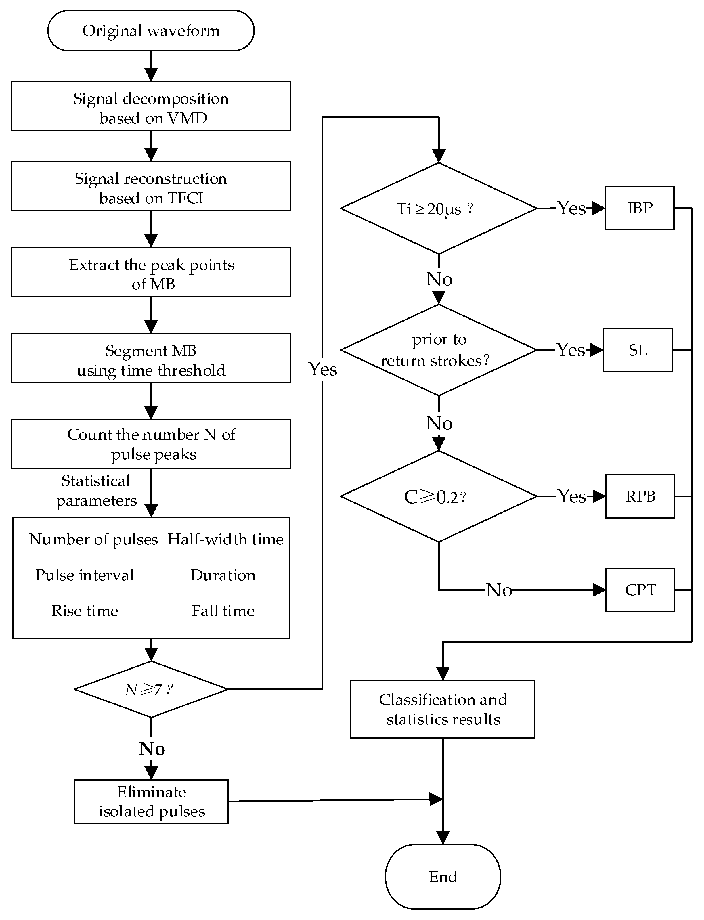
To address the aforementioned issues, VMD is employed to decompose the VLF/LF electric field waveforms of lightning into multiple intrinsic mode functions (IMF). Subsequently, the Trend-Free Correlation Index (TFCI) is applied to screen and retain appropriate intrinsic mode functions. TFCI involves calculating the correlation coefficients between each IMF and the original signal on an individual basis. Subsequently, signal reconstruction is carried out by utilizing only those IMFs whose correlation coefficients exceed the mean value of all computed correlation coefficients, thereby achieving signal detrending. This process effectively removes slowly varying low-frequency components and relatively high-frequency noise. This thus provides the possibility of determining the pulse peaks based on the comparison of amplitude features. However, some broadband background noise remains in the retained useful signals. To mitigate this, the pulse threshold can be set as twice the average amplitude of the noise. By establishing criteria such as the minimum peak height, the minimum relative peak height difference, and the minimum peak interval, effective pulse peak points can be identified. Furthermore, by defining the minimum pulse time interval threshold, portions of the pulse sequence in time can be extracted, allowing for the statistical analysis of the number of pulse peaks and related time-domain parameters within these portions.

If the number of pulses within a segment is fewer than 7 (the multiple burst exhibits a repetition count of 20 [1]), the pulse group is categorized as an isolated pulse discharge event, and no further statistical analysis is performed. According to the statistical results of predecessors, the pulse intervals of RPB, CPT, and DL are usually several microseconds [3,35,36,37], and the pulse interval time of an IBP typically ranges from tens of microseconds to one hundred microseconds [18,30,38,39], with the pulse repetition count varying between several and dozens. Consequently, based on the overall distribution pattern of the time-domain parameters of RPs, the following identification process can be established:

If the pulse count exceeds 7 and the average pulse interval exceeds 20 μs, it is classified as an IBP. If the average pulse interval is less than 20 μs and the pulse sequence is immediately followed by a return stroke process, it is identified as a dart-stepped leader. If the pulse group is not immediately followed by a return stroke process and the similarity coefficient C between adjacent pulses is larger than 0.2, indicating high overall waveform similarity and regularity, it is classified as an RPB; otherwise, it is categorized as a CPT. Subsequently, the time-domain characteristic parameters of each type of repetitive pulse discharge event are statistically analyzed. The analysis process is illustrated in Figure 8.

3.2. Signal Decomposition Based on VMD

The VMD algorithm is a frequency-domain signal decomposition method that has been widely applied to the processing of time-varying non-stationary signals. Its core principle involves constructing and solving variational optimization problems. As a non-recursive algorithm, it can efficiently achieve the global optimal solution, thereby effectively avoiding mode mixing and endpoint effects. Additionally, it exhibits strong robustness against noise and achieves superior mode separation performance [40].

VMD first constructs a variational problem, and based on the preset number of scales N, derives N mode functions with specific center frequencies ${\omega }_n$. To estimate the bandwidth of each mode function $u_n$, the Hilbert transform is applied to obtain the single-sided spectrum of each mode function $u_n$. Subsequently, the exponential mixed modulation method is employed to shift the spectrum of each mode to its estimated center frequency. Finally, the bandwidth estimation is accomplished through signal demodulation using the gradient square criterion and Gaussian smoothing.

The formulation of the constrained variational problem is presented as follows:

$${\min }_{\left\{u_n\right\},\left\{{\omega }_n\right\}}\left\{{\displaystyle \sum _n{‖{\partial }_t\left[\left(\delta (t)+\frac{j}{\pi t}\right)u_n(t)\right]e^{-j{\omega }_{n}t}‖}_2^2}\right\}$$

(1)

$${\displaystyle \sum _n{u}_n}=f$$

(2)

By introducing the Lagrange multiplier $\lambda \left(t\right)$ and the quadratic penalty factor $\alpha$, the constrained variational problem is reformulated as an unconstrained variational problem, and the augmented Lagrangian expression is derived accordingly:

$$\begin{array}{l}L\left(\left\{u_n\right\},\left\{{\omega }_n\right\},\lambda \right)=\alpha {\displaystyle \sum _n{‖{\partial }_t\left[\left(\delta (t)+\frac{j}{\pi t}\right)u_n(t)\right]e^{-j{\omega }_{\sigma }t}‖}_2^2}+{‖f\left(t\right)-{\displaystyle \sum _n{u}_n}\left(t\right)‖}_2^2+〈\lambda \left(t\right),f\left(t\right)-{\displaystyle \sum _n{u}_n}\left(t\right)〉\\ \end{array}$$

(3)

The alternating direction method of multipliers is employed to iteratively update variables $u^{n+1},{\omega }_n^{n+1},{\lambda }^{n+1}$ and locate the saddle point of the aforementioned equation. The detailed procedures are presented below:

• Initialize the parameters ${\widehat{u}}^1,{\omega }^1,{\widehat{\lambda }}^1$ and set the maximum number of iterations $k=0$;
• Increment the iteration counter $k=k+1$;
• For each decomposition scale $1\le n\le N$, compute Formulas (4) and (5), and update variables ${\widehat{u}}_n$ and ${\omega }_n$ when $\omega \ge 0$;

  $${\widehat{u}}_n^{k+1}(\omega )={\displaystyle \frac{\widehat{f}(\omega )-{\displaystyle \sum _{i=n}^N{\widehat{u}}_n^{k+1}}(\omega )+{\widehat{\lambda }}^k\left(\omega \right)/2}{1-2\alpha {\left(\omega -{\omega }_n^k\right)}^2}}$$

  (4)

  $${\omega }_n^{k+1}={\displaystyle \frac{{\displaystyle {\int }_0^{\infty }\omega }{\left|{\widehat{u}}_n^{k+1}(\omega )\right|}^{2}d\omega }{{\displaystyle {\int }_0^{\infty }{\left|{\widehat{u}}_n^{k+1}\left(\omega \right)\right|}^2}d\omega }}$$

  (5)

  where ${\widehat{u}}_n^{k+1}\left(\omega \right)$, $\widehat{f}(\omega )$, and ${\widehat{\lambda }}_n^{\widehat{\kappa }+1}(\omega )$ are the Fourier transforms of their respective time-domain functions.
• Update $\lambda$ by applying enhancement when $\omega \ge 0$ according to the formula below:

  $${\widehat{\lambda }}^{k+1}(\omega )={\widehat{\lambda }}^k\left(\omega \right)+\tau \left[\widehat{f}(\omega )-{\displaystyle \sum _{n=1}^N{\widehat{u}}_n^{k+1}}(\omega )\right]$$

  (6)

  where $\tau$ denotes the noise tolerance.
• Iterate through the above steps until the stopping condition is satisfied:

  $${\displaystyle \sum _n\left({‖{\widehat{u}}_n^{k+1}-{\widehat{u}}_n^k‖}_2^2/{‖{\widehat{u}}_n^k‖}_2^2\right)}<\epsilon$$

  (7)

  where $\epsilon >0$ and denotes the convergence accuracy. Finally, N intrinsic mode functions are obtained, thereby concluding the iterative update process.

When applying VMD, two critical parameters must be determined: the number of decomposition modes $N$ and the penalty factor $\alpha$. These parameters significantly influence the VMD performance. Setting N too high may cause over-decomposition, leading to invalid redundant information; setting N too low may result in mode aliasing. Regarding the penalty factor $\alpha$, a larger value narrows the bandwidth of IMFs, potentially causing distortion, while a smaller value widens the bandwidth of IMFs, making it more susceptible to noise interference. In this study, the penalty factor is set to $\alpha =4000$, and the number of decomposition modes is set to $N=8$.

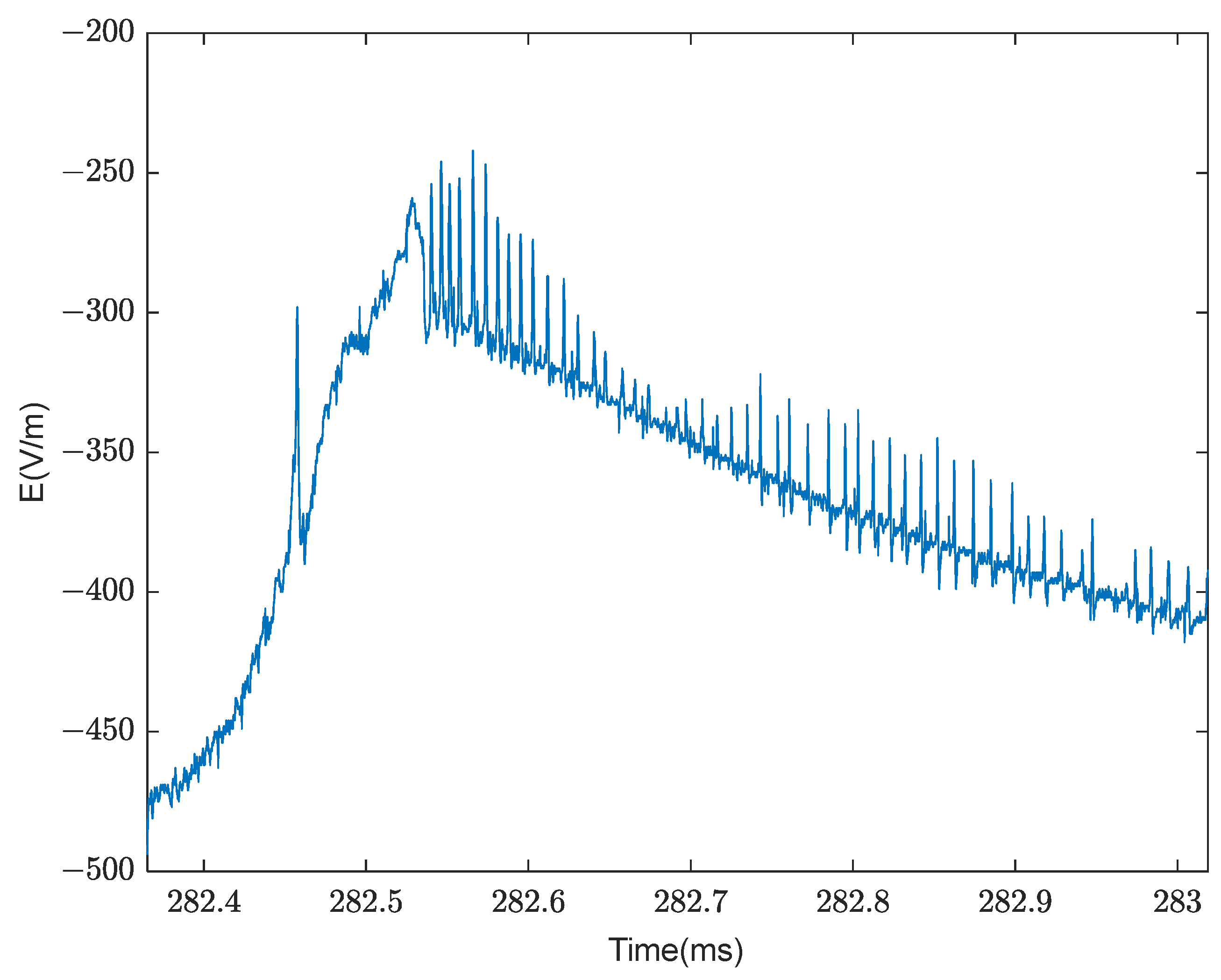
Figure 9 illustrates a set of typical RPB events superimposed on the trailing edge of a slowly varying K change. Owing to the presence of abundant low-frequency components, accurately extracting the pulse peak based solely on amplitude features presents significant challenges.

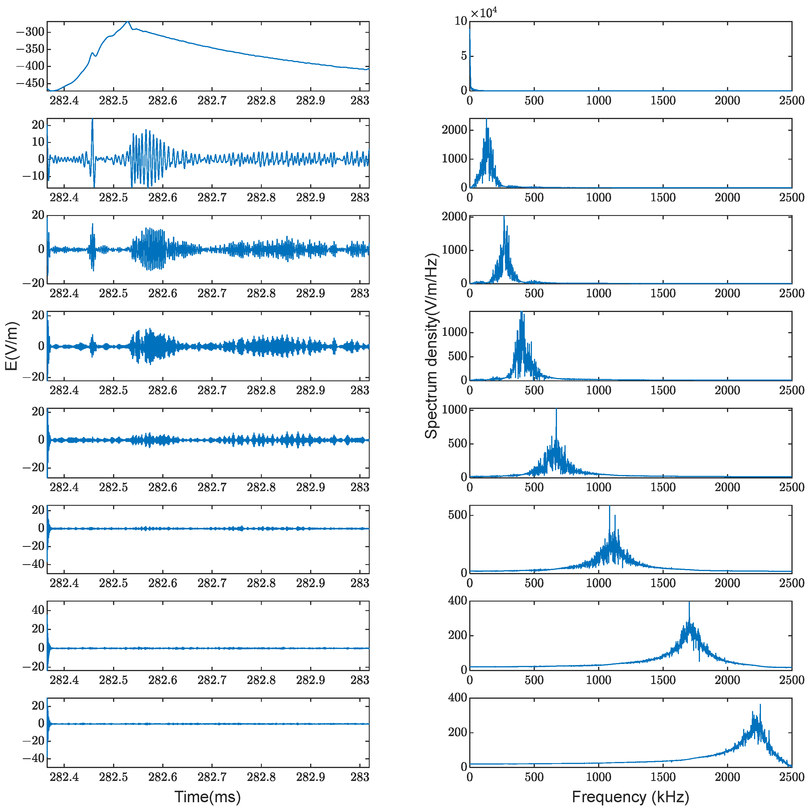
Figure 10 presents the time-domain and frequency-domain decomposition results of the 8 IMF components obtained after VMD processing. It is evident that each modal component has been successfully separated in order from low frequency to high frequency.

3.3. Signal Reconstruction Based on TFCI

The correlation between each component and the original signal is assessed using the correlation analysis method. Let ${\rho }_{\mathrm{i}}$ denote the correlation coefficient between the i-th IMF component and the original signal, and its calculation formula is as follows:

$${\rho }_i={\displaystyle \frac{{\displaystyle \sum _{i=1}^{Num}\left(x_k-\overline{x}\right)}\left(d_{ik}-\overline{d_i}\right)}{\sqrt{{\displaystyle \sum _{k=1}^{Num}{\left(x_k-\overline{x}\right)}^2}{\displaystyle \sum _{k=1}^{Num}{\left(d_{ik}-\overline{d_i}\right)}^2}}}}(i=1,2,\cdots ,n)$$

(8)

In this equation, $Num$ denotes the total number of data points in the signal, $x_k$ denotes the k-th data point of the signal, $\overline{x}$ denotes the mean value of the signal, $d_{ik}$ denotes the k-th data point of the i-th IMF component, and ${\overline{d}}_i$ denotes the mean value of all data points of the i-th IMF component. By setting $N=8$, the correlation coefficients between each mode component and the original signal are presented in

Table 1. Correlation coefficients between each IMF and the original signal.

IMF Component	Correlation Coefficients
IMF1	0.9868
IMF2	0.1168
IMF3	0.0935
IMF4	0.0792
IMF5	0.0451
IMF6	0.0231
IMF7	0.0178
IMF8	0.01670

.

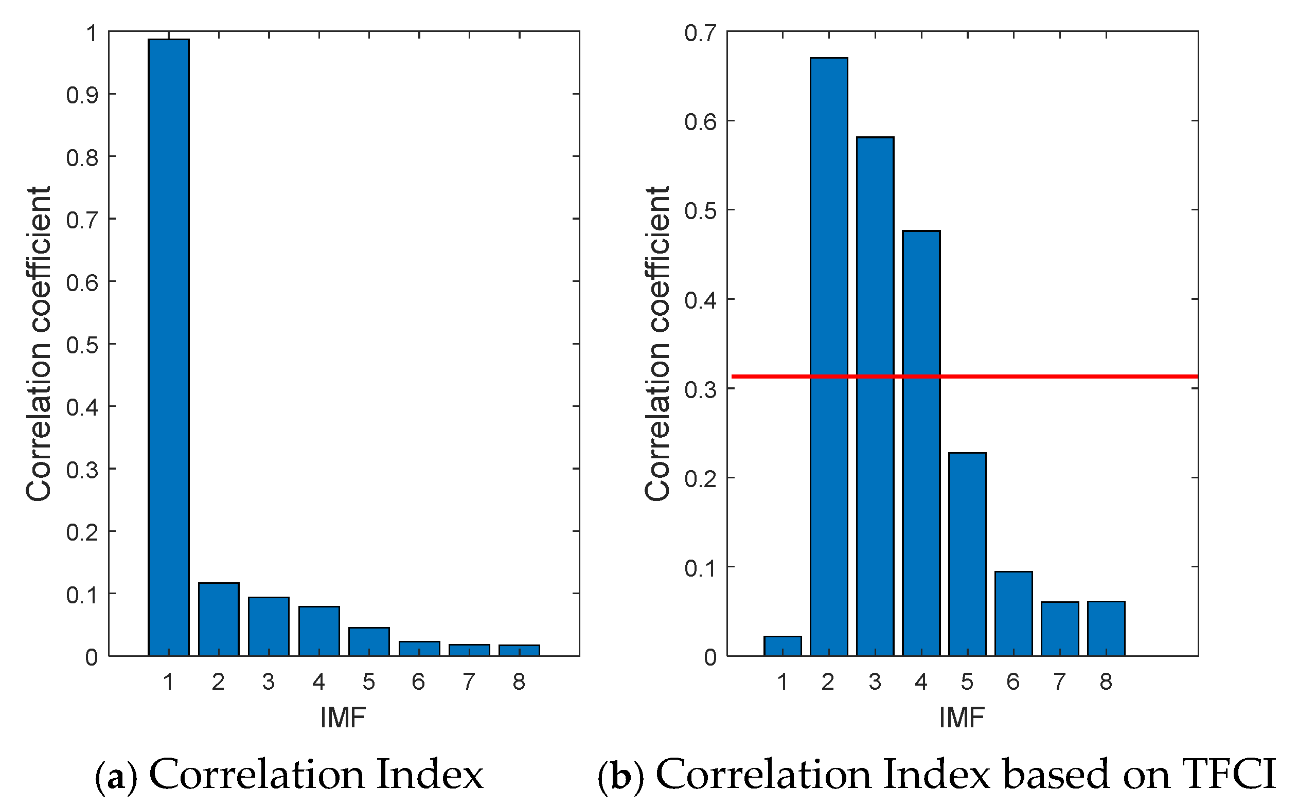
It can be observed that for electric field signals with slowly varying and superimposed pulse components, the presence of the slowly varying trend component IMF1 causes the characteristics of the original signal to be predominantly determined by this component. As a result, the correlation index becomes ineffective in distinguishing other components. To address this issue, this paper introduces the trend-free correlation index (TFCI), where $u_{trend}$ denotes the trend component, $x^{\prime }$ denotes the new signal used to replace the original signal $x$, $u\left(i\right)\left(i=1,2,\cdots ,z\right)$ denotes the i-th component, and $z$ denotes the total number of decomposed modes. Specifically,

$$u_{trend}=u\left(1\right)$$

(9)

$$x^{\prime }=u\left(2\right)+u\left(3\right)+\cdots +u\left(z\right)$$

(10)

Subsequently, the detrended cross-correlation coefficient can be formulated as

$${{\rho }_i}^{\prime }={\displaystyle \frac{{\displaystyle \sum _{i=1}^{Num}\left(x_k^{\prime }-\overline{x^{\prime }}\right)}\left(d_{ik}-\overline{d_i}\right)}{\sqrt{{\displaystyle \sum _{k=1}^{Num}{\left(x_k^{\prime }-\overline{x^{\prime }}\right)}^2}{\displaystyle \sum _{k=1}^N{\left(d_{ik}-\overline{d_i}\right)}^2}}}}(i=1,2,\cdots ,n)$$

(11)

Table 2. Correlation coefficients between each IMF and the detrended original signal.

IMF Component	Correlation Coefficients
IMF1	0.0218
IMF2	0.6704
IMF3	0.5811
IMF4	0.4763
IMF5	0.2273
IMF6	0.0943
IMF7	0.0603
IMF8	0.0608

lists the detrended cross-correlation index values between each modal component and the original signal, while Figure 11 illustrates the comparative effectiveness of the correlation index and the detrended cross-correlation index in distinguishing meaningful components, the red line in Figure 11b denotes the mean of the correlation coefficients.

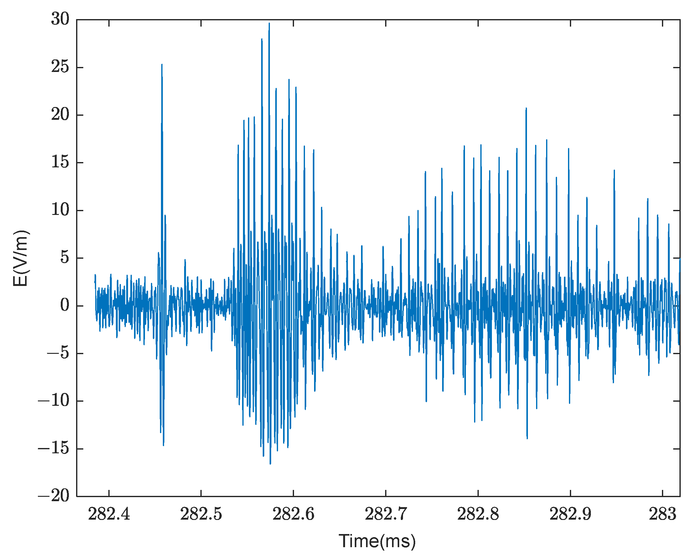
The average value of the detrended cross-correlation index is used as the threshold to select the second, third, and fourth IMF components for reconstructing the lightning signal. The time-domain waveforms are presented in Figure 12, where it can be observed that the low-frequency trend term and high-frequency noise of the impulse group signal have been effectively suppressed.

3.4. Time-Domain Feature Analysis

3.4.1. Time-Domain Feature Analysis of RPB

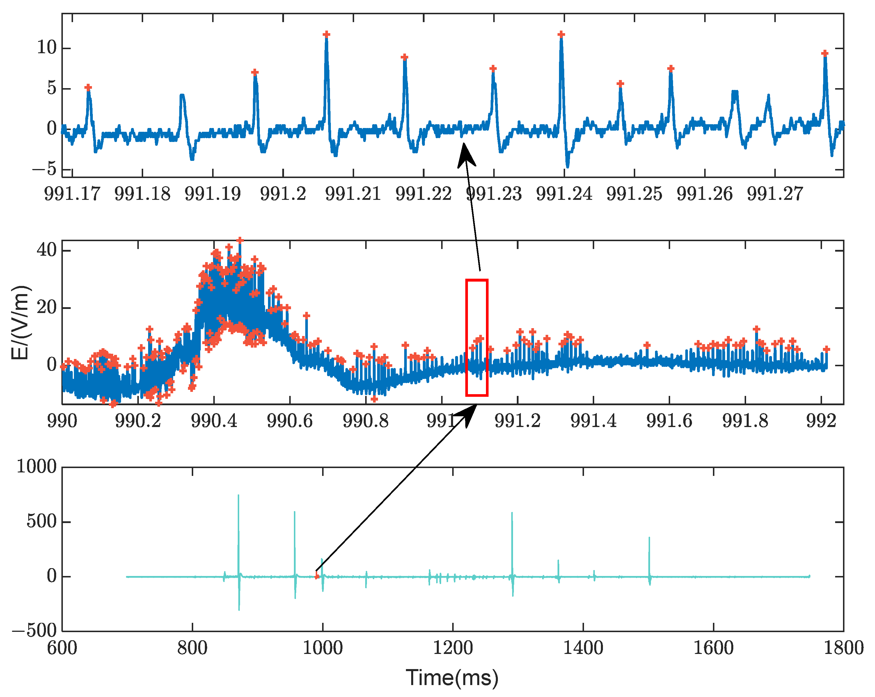
The paper collected a total of 352 RPB sequence samples, from which 29,724 individual pulses were extracted. A representative sample is presented in Figure 13, the red plus signs denote the extracted pulse peaks, and this notation is consistently applied throughout the subsequent text unless otherwise specified. It is relatively straightforward to observe that most of the individual pulses demonstrate a distinct bipolar characteristic, with the amplitude of the first half-cycle being substantially larger than that of the second half-cycle.

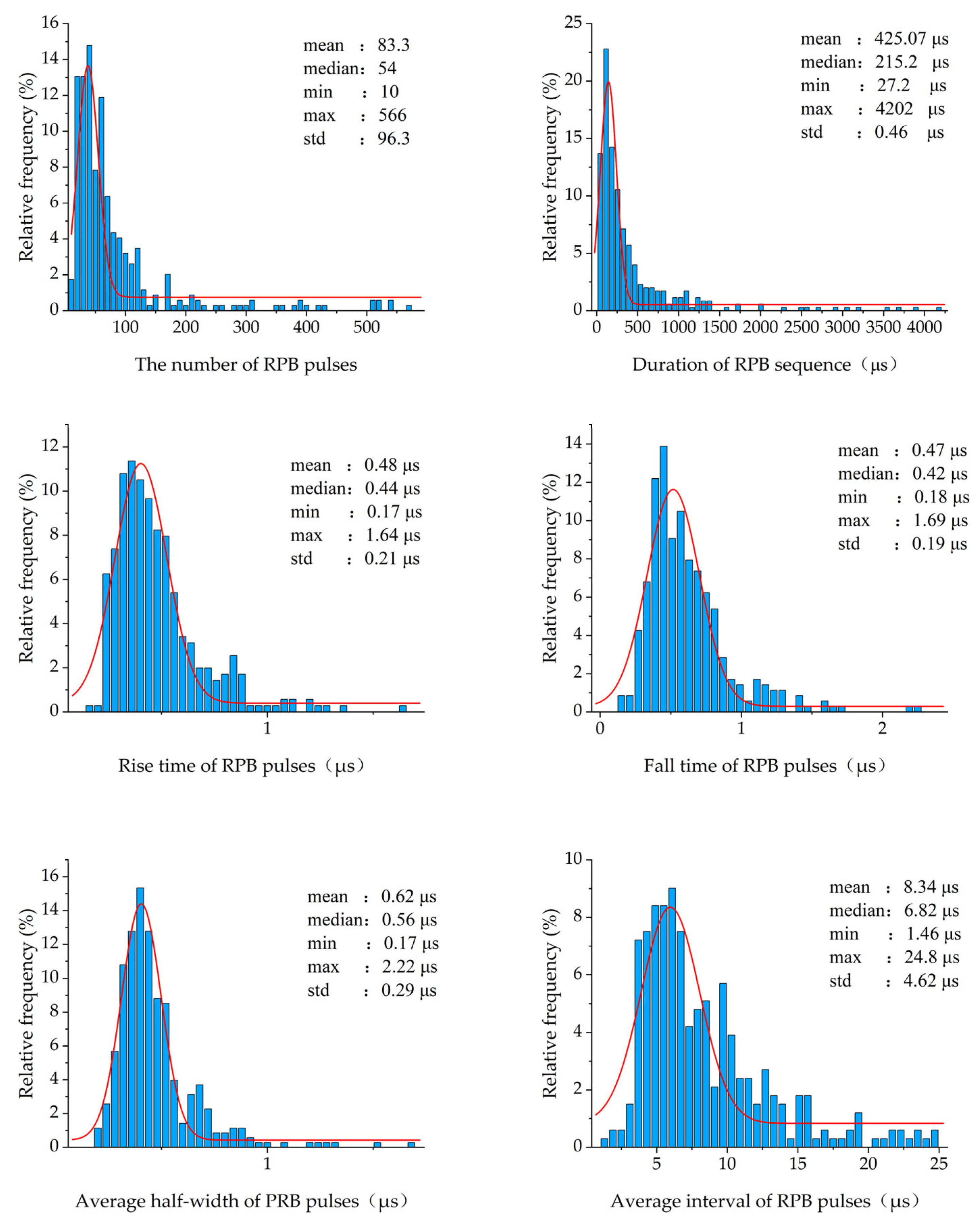
As shown in Figure 14, the statistical results indicate that the pulse burst duration ranges from 27.2 μs to 4202 μs (with an average of 425.07 μs and a median of 215.2 μs), the pulse repetition count varies between 10 and 566 (with an average of 83.3 and a median of 54), the average half-width time of a single pulse is within 0.17 μs to 2.22 μs (with an average of 0.62 μs and a median of 0.56 μs), the average pulse interval time spans from 1.46 μs to 24.8 μs (with an average of 8.34 μs, and a median of 6.82 μs), the average rise time is between 0.17 μs and 1.64 μs (with an average of 0.48 μs and a median of 0.44 μs), and the average fall time ranges from 0.18 μs to 1.69 μs (with an average of 0.47 μs and a median of 0.42 μs).

Through statistical analysis of the observational data and the comparison with the conclusions drawn by domestic and international observation teams, it was found that the time-domain parameters of regular pulse groups are largely consistent with existing sporadic statistical results. However, some data distribution ranges are broader than those reported in previous studies, which may be attributed to variations in sample size, differences in geographical environment, and the bandwidth and precision limitations of the testing equipment.

3.4.2. Time-Domain Feature Analysis of CPT

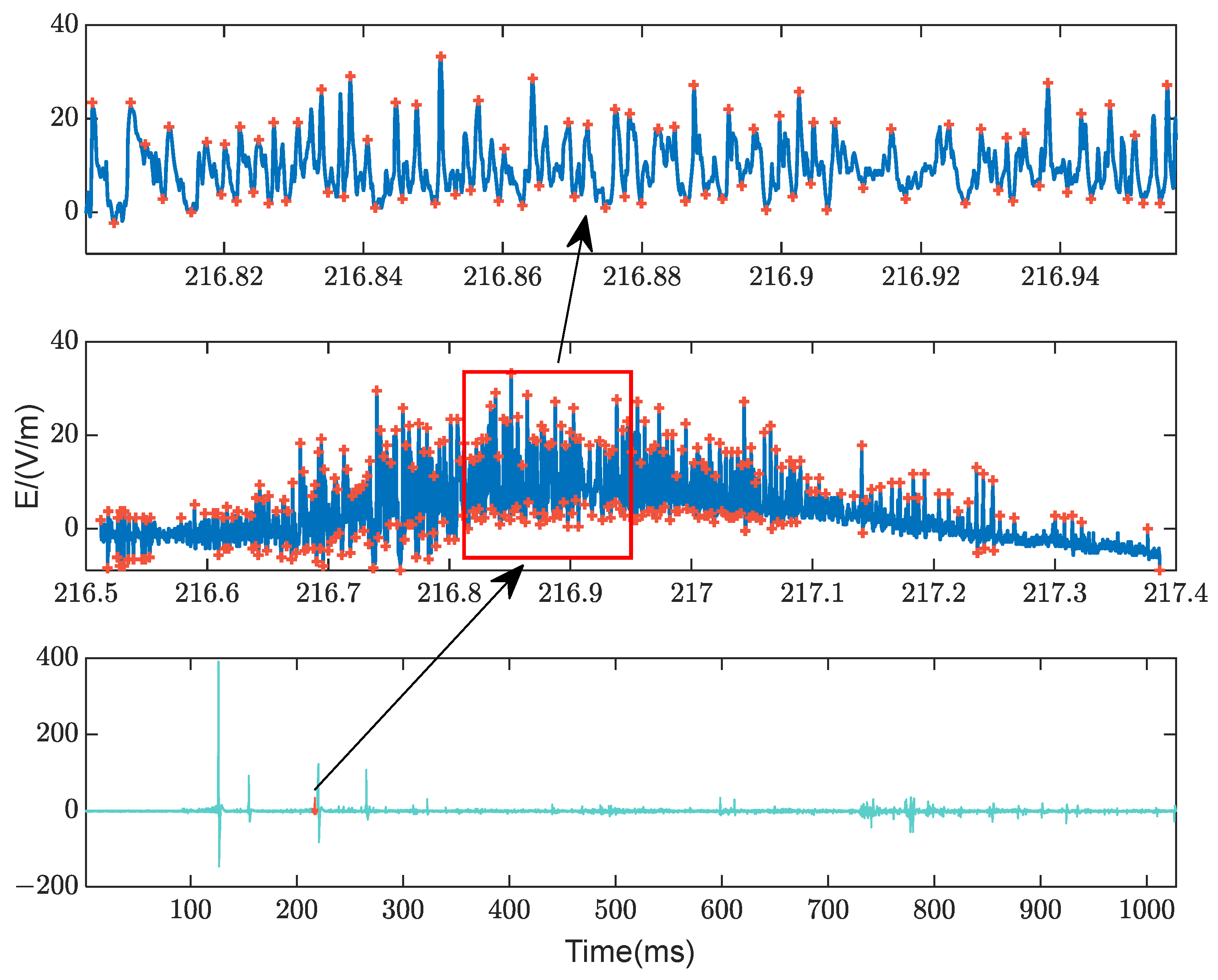
A typical CPT time-domain waveform is presented in Figure 15. Given the irregularity of the pulse shape, pulse width, and pulse peak in the CPT pulse train, it is challenging to accurately determine the start and end times of each pulse. Nevertheless, by setting a threshold at twice the noise level, the pulse train data segment can be extracted, and the average time-domain parameters can then be statistically analyzed. Due to the inherent irregularities of the CPT waveform, significant individual variations still exist in the average time-domain parameters.

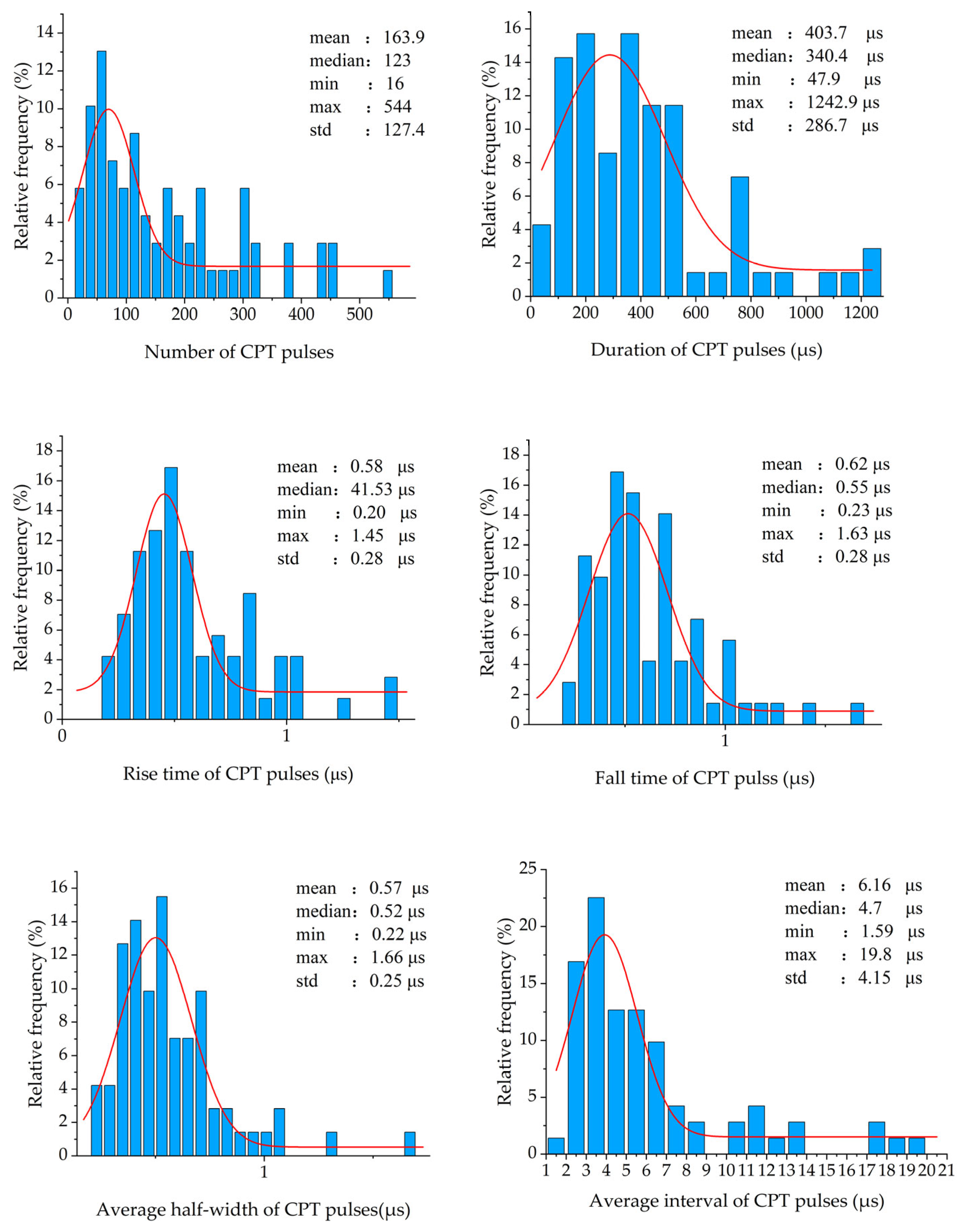
Based on 72 CPT sequence samples, a total of 12,030 single-pulse samples were identified. Statistical analysis reveals that the number of pulses in a CPT pulse sequence ranges from 16 to 544 (with an average of 163.9 and a median of 123), the pulse sequence duration spans from 47.9 μs to 1242.9 μs (with an average of 403.7 μs and a median of 340.4 μs), the average pulse interval time varies between 1.59 μs and 19.80 μs (with an average of 6.16 μs and a median of 4.7 μs), the average pulse half-width time is within the range of 0.22 μs to 1.66 μs (with an average of 0.57 μs and a median of 0.52 μs), the rise time ranges from 0.2 μs to 1.45 μs (with an average of 0.58 μs and a median of 41.53 μs), and the fall time is between 0.23 μs and 1.63 μs (with an average of 0.62 μs and a median of 0.55 μs). These statistical results are illustrated in Figure 16.

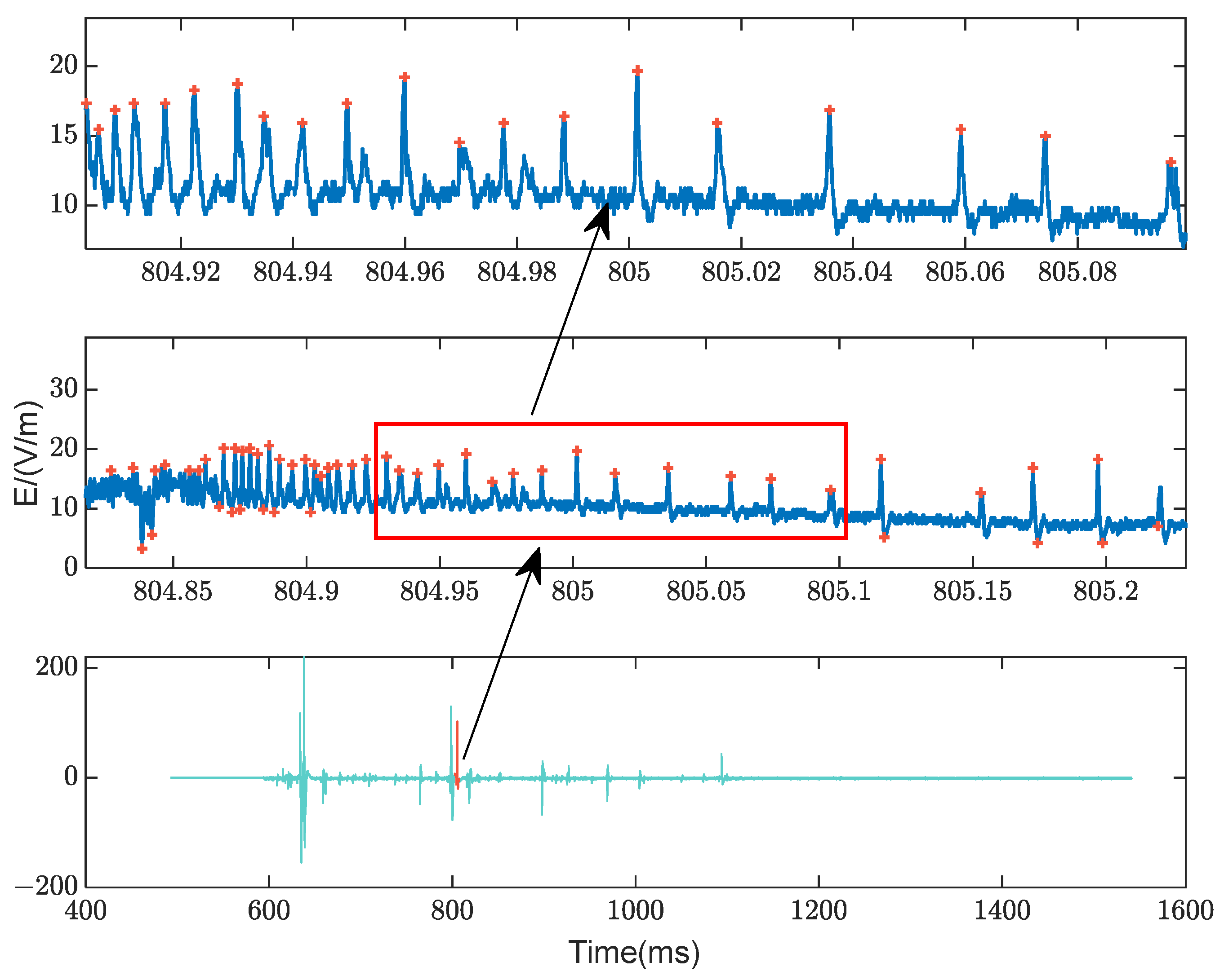
3.4.3. Time-Domain Feature Analysis of DSL

A total of 248 dart-stepped leader sequence samples were analyzed, and 120,063 single pulse samples were identified. A typical DSL time-domain waveform is presented in Figure 17.

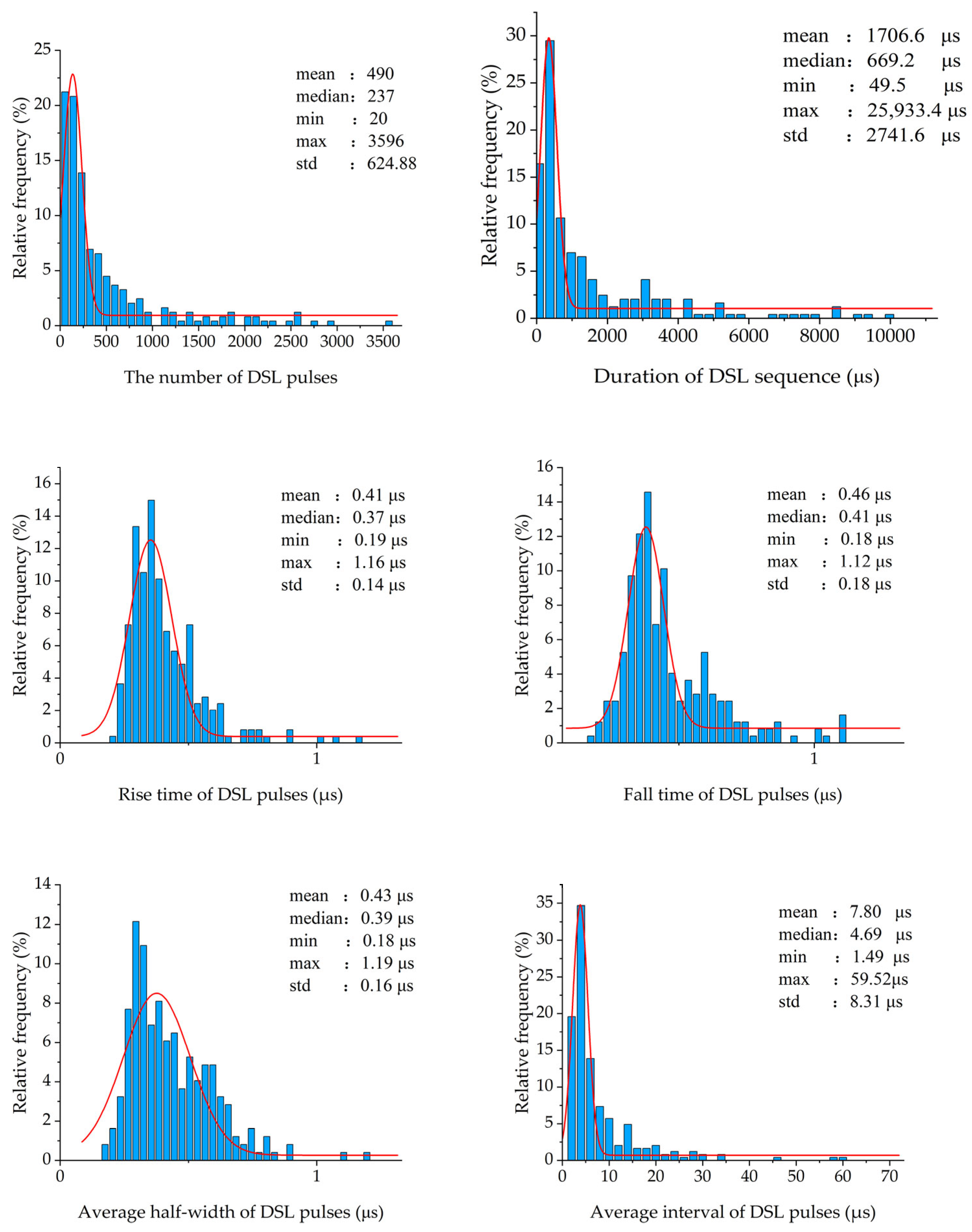
The pulse repetition count within the pulse train varies between 20 and 3596 pulses (average: 490 pulses, median: 237 pulses). The pulse sequence duration ranges from 49.5 μs to 25,933.4 μs (average: 1706.6 μs, median: 669.2 μs). The average half-width of a single pulse is between 0.18 μs and 1.19 μs (average: 0.43 μs, median: 0.39 μs). The average pulse interval time ranges from 1.49 μs to 59.52 μs (average: 7.8 μs, median: 4.69 μs). Additionally, the average rise time is from 0.19 μs to 1.16 μs (average: 0.41 μs, median: 0.37 μs), and the average fall time is between 0.18 μs and 1.12 μs (average: 0.46 μs, median: 0.41 μs). These statistical results are presented in Figure 18.

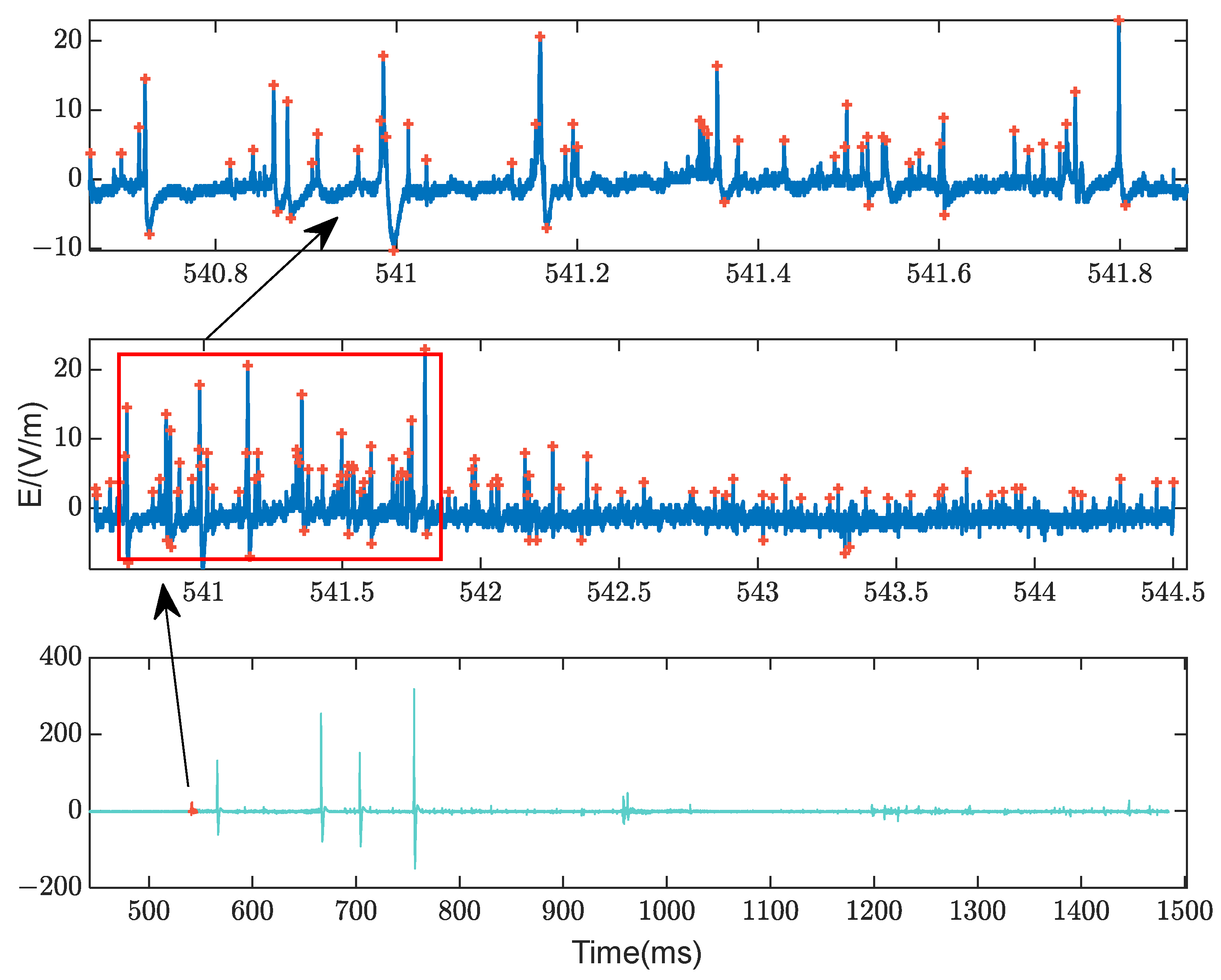
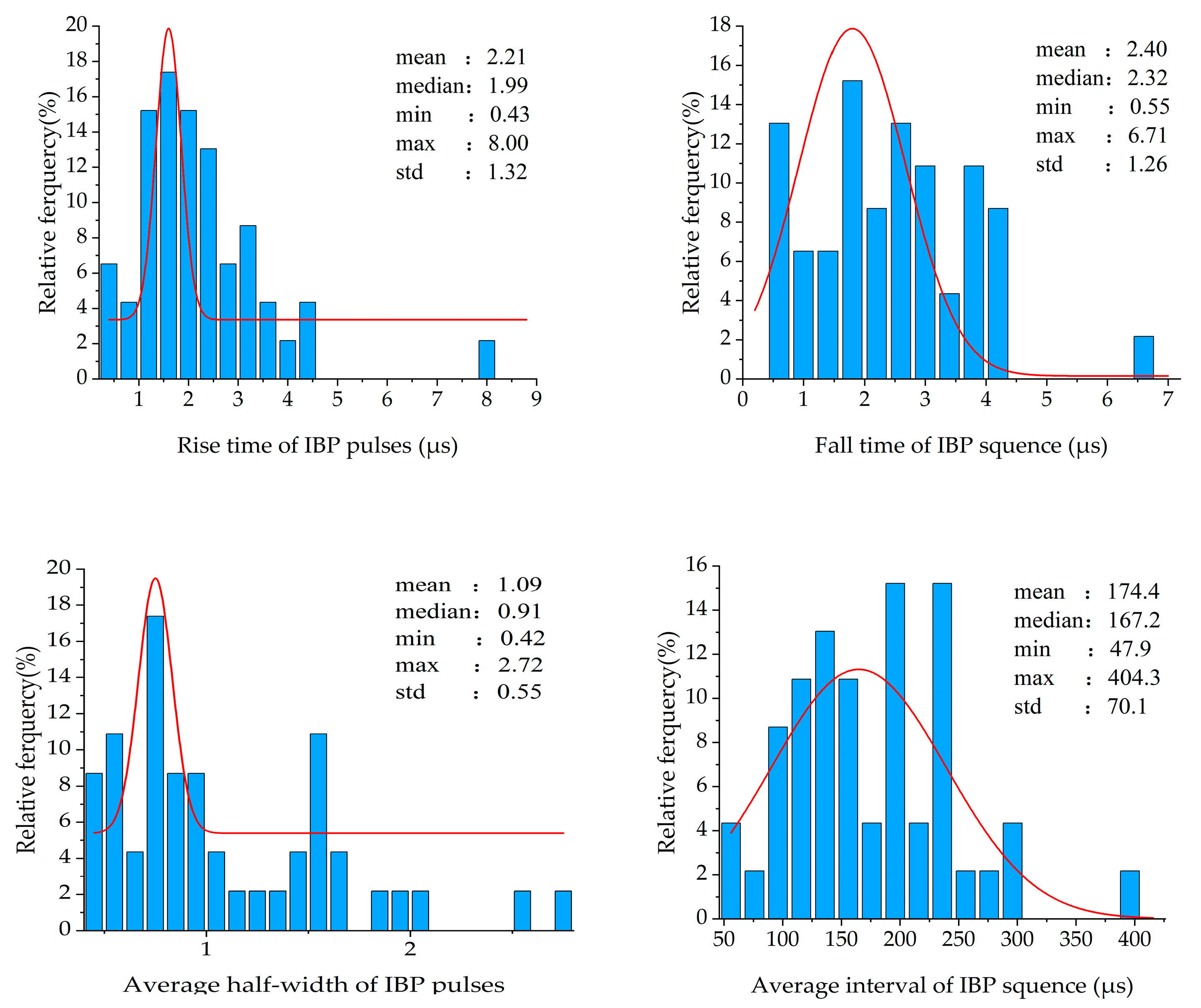
3.4.4. Time-Domain Feature Analysis of IBP

During the experiment, we collected a total of 46 IBP sequence samples, from which 1752 individual pulses were extracted. A representative sample is presented in Figure 19. Similar to the RPB sample presented in Figure 13, the IBP pulses also demonstrate a distinctly bipolar characteristic. In particular, this is evident in individual pulses with relatively large amplitudes, where the second half-cycle is more pronounced.

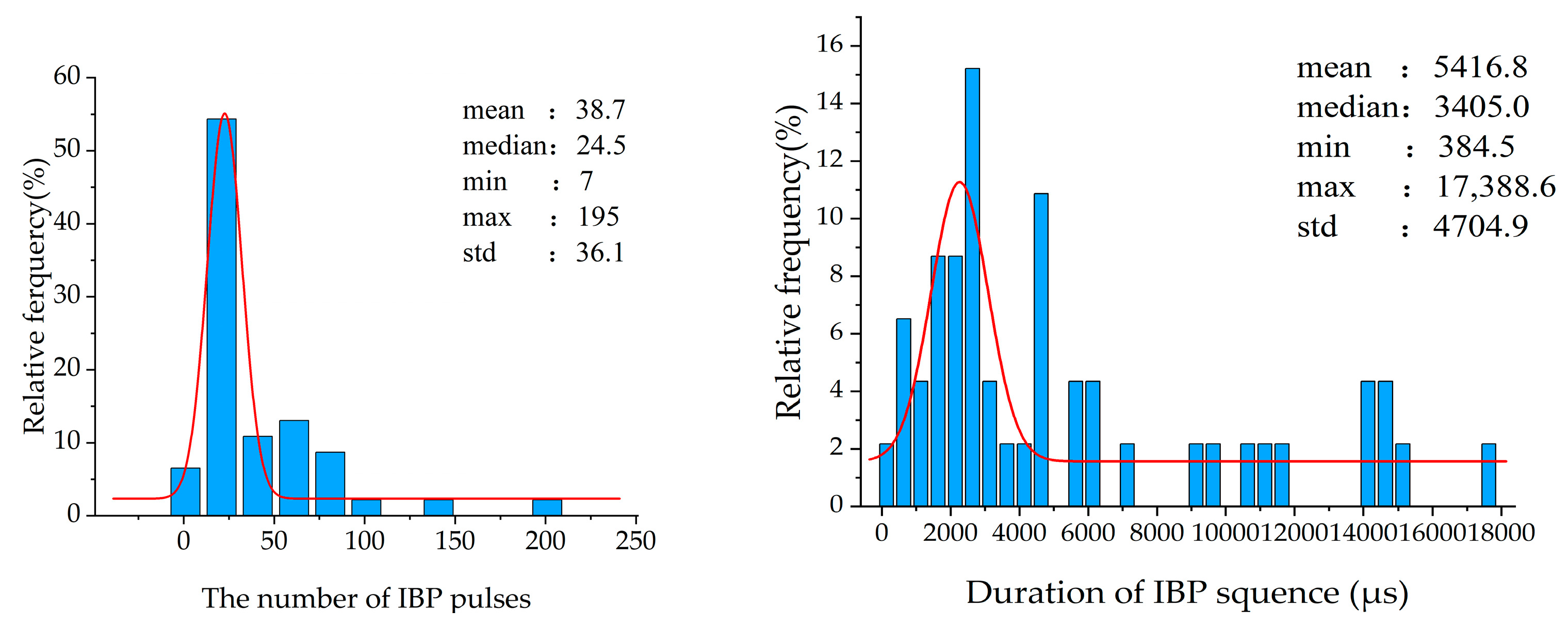
The repetition count of IBPs ranges from 7 to 195 (with an average of 38.7 and a median of 24.5), following a normal distribution overall. The pulse sequence duration spans from 384.5 μs to 17,388.6 μs (with an average duration of 5416.8 μs), also exhibiting a normal distribution. The average pulse interval time varies between 47.9 μs and 404.3 μs (with an average of 174.4 μs). Approximately 93.4% of the samples have a half-width time within 2 μs. The rise time exhibits a distribution within the interval of 0.43 to 0.8 μs, with a mean value of 2.21 μs and a median of 1.99 μs. The fall time demonstrates a distribution ranging from 0.55 to 6.71 μs, featuring an average of 2.4 μs and a median of 2.32 μs. These statistical results are illustrated in Figure 20.

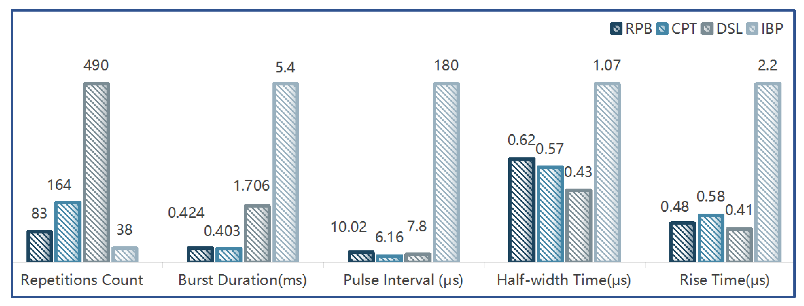
Based on the aforementioned statistical analysis, Figure 21 presents a comparative evaluation of the average time-domain parameter values for RPB, CPT, DSL, and the IBP. DSL exhibits stepwise development within the pre-established lightning return stroke channel, which can extend several kilometers in length. Consequently, it demonstrates the longest burst duration and the largest pulse repetition count. An IBP typically occurs during the initial phase of lightning activity, prior to the formation of the leader discharge channel, resulting in the longest pulse interval and pulse rise time. Furthermore, when considering parameters such as pulse interval, half-width time, and rise time, the waveforms of RPB and DSL exhibit significant similarity.

4. Comparison of Time-Domain Characteristics of Repetitive Pulse Discharge Events and MB Test Environments

The current definition of the multiple burst test environment was revised by the SAE committee in 1990 and has been used since then. The main revisions are as follows: (1) the number of pulse bursts per lightning strike was reduced from 24 to 3; (2) the pulse interval was extended from 10–50 μs to 50–1000 μs; and (3) the interval between pulse bursts was adjusted from 10–200 ms to 30–300 ms. The number of pulses in a single pulse burst (20) and the time-domain waveform of individual pulses remain unchanged.

Rakov et al. [3] noted that the 1990-revised definition of multiple burst is closer to the characteristics of the IBP, whereas the original definition aligns better with RPB. However, this conclusion was based solely on the parameter of pulse interval and lacks comprehensive and accurate data support for validation.

Table 3. Comparison of time-domain characteristics of repetitive pulse discharge events and MB test environments.

RP	Reference	Number of Bursts	Repetitions Count	Burst Duration (ms)	Pulse Interval (μs)	Half-Width Time (μs)	Rise Time (μs)
MB Definition	SAE ARP 5412C [1]	—	20	1~20	50~1000	4	0.245
RPB	Krider, E.P. [5]	—	—	0.1~0.4	6.1	0.75	—
	Rakov, V.A. [3]	162	68	0.29	11.3	—	0.75
	Davis, S.M. [35]	—	—	—	2.8~5.1	—	—
	Kolmasova, I. [8]	33	39	0.176	4.7	—	—
	Fan, X.P. [41]	1	101	0.89	—	—	1.93
	SLOT	353	83	0.424	10.02	0.62	0.48
CPT	Lan, Y. [12]	65	—	0.47	—	—	—
	Gomes, C. [4]	—	—	0.4~0.5	—	2~20	—
	Mäkelä, J.S. [10]	26	—	0.29	—	—	—
	Willett, J.C. [42]	15	—	—	—	2~4	—
	SLOT	72	164	0.403	6.16	0.57	0.58
DSL	Qi, Q. [43]	9	—	—	17.4	—	—
	Krider, E.P. [44]	17	8	—	16	0.4~0.5	0.3
	Rakov, V.A. [3]	—	—	—	6~8	1~2	—
	Qie, X.S. [22]	4	108	7.7	12.2	0.5	—
	Li, H. [45]	12	—	1.689	—	—	—
	Qie, X.S. [37]	45	—	—	15.8	—	—
	SLOT	247	490	1.706	7.80	0.43	0.41
IBP	Yoshida, S. [30]	35	—	2.7	73	—	—
	Nag, A. [46]	12	—	3.4	65	—	—
	Baharudin, Z.A. [18]	24	—	12.3	152	—	—
	Karunarathne, S. [38]	6	—	—	—	—	12
	Shi, D.D. [32]	46	—	0.19	—	3	10.5
	Karunarathne, N. [31]	29	—	—	—	—	15.04
	Thottappillil, R. [39]	—	—	—	100	—	—
	Cao, D.J. [33]	24	54	—	—	—	—
	SLOT	46	39	5.4	174	1.09	2.2

presents a comparison between the MB parameter definitions and the data obtained from this study as well as prior observations, with the bold sections highlighting the statistical findings of our SLOT team.

In terms of pulse repetition count, the four types of repetitive pulse discharge events—IBP, RPB, CPT, and DSL—all significantly exceed the 20 pulses defined in the MB test environment. Regarding burst duration, the IBP and DSL are closer to the MB test environment’s definition. In terms of pulse interval time, the intervals for RPB, CPT, and DSL are at the microsecond scale, whereas the interval for the IBP aligns more closely with the MB test environment definition. With respect to rise time, the rise edges of RPB, CPT, and DSL are steeper, indicating characteristics of fast leading edges.

By comparison, it is evident that the MB parameter definition does not precisely align with any specific natural lightning repetitive pulse discharge event but instead integrates the primary characteristics of several common repetitive pulse discharge events. Consequently, the MB parameter definition can be interpreted as a generalization and synthesis of the protection requirements for these common repetitive pulse discharge events during the occurrence and development of lightning. This serves to evaluate the indirect effects on aircraft and their associated equipment in a multi-pulse discharge environment.

5. Conclusions

In order to clarify the relationship of MBs defined in lightning test standards with the observation data of RPs, field measurement and data analysis are carried out in this research. Natural lightning data were decomposed and reconstructed using the VMD method based on TFCI; subsequently, RP samples were identified and extracted based on the characteristics of the number of repetitions and amplitude. A comprehensive statistical analysis of 719 RPs (including a total of 163,589 single pulses) and multiple parameters was conducted to characterize the time-domain features of microsecond-scale repetitive discharge events in natural lightning. These findings were compared and validated against the sporadic statistical results reported by previous studies.

The conclusion shows that, considering time-domain parameters such as pulse repetition count, pulse sequence duration, half-width time, pulse interval time, and rise time, the standard parameters defined for the MB test environment do not precisely align with any specific natural lightning repetitive discharge event. Instead, they integrate the key features of several common repetitive pulse discharge events. Consequently, these parameters can be interpreted as a synthesis and generalization of protection requirements for typical repetitive pulse discharge events during the occurrence and development of lightning, enabling the assessment of indirect effects on aircraft and their associated equipment in a multi-pulse discharge environment.

Based on the results of the comparative analysis, targeted revision suggestions for the MB test environment standard are proposed as shown in Figure 22:

• The defined pulse interval by the MB test environment standard is 50 to 1000 μs, while observed data predominantly fall within the range of several microseconds to tens of microseconds. It is advisable to shorten the defined interval to the microsecond range.
• The defined pulse repetition count by the MB test environment standard is 20 pulses, whereas observed data range from 39 to 486 pulses. It is recommended to increase the defined repetition count to the order of hundreds.
• The defined pulse half-width time by the MB test environment standard is 4 μs; however, the four types of RPs half-width times analyzed statistically by previous studies and in this paper are predominantly within the range of 1 to 2 μs or at the sub-microsecond level. Therefore, it is reasonable to consider reducing the defined half-width time to 2 μs.
• An IBP typically exhibits the characteristics of a bipolar pulse, with a relatively larger peak current and longer duration. Consequently, when defining a single-Component H waveform, the potential impact on aircraft should be taken into account. It may be advisable to revise the unipolar representation of Component H waveforms to incorporate bipolar characteristics. Cao et al. conducted a statistical analysis of measured IBP waveforms and discovered that the peak value of the initial half-cycle for the majority of the bipolar IBP is significantly higher than the peak value of the opposite polarity in the subsequent half-cycle, with an amplitude ratio exceeding 2. Additionally, the rising edge of the initial half-cycle waveform exhibits a relatively steep slope [33]. This paper selected 64 IBP single-pulse samples and calculated the amplitudes of the half-cycle with the relatively larger peak and the half-cycle with the opposite polarity. It was found that the average ratio of the two amplitudes was 0.31, which is consistent with the results of Cao et al. Based on these findings, the negative half-cycle current peak of the H-wave can be set to 3 kA while maintaining the rise time of the initial half-cycle unchanged.