
Long-Term Pre-Diagnosis Exposure to Ambient Air Pollution and Weather Conditions and Their Impact on Survival in Stage 1A Non-Small Cell Lung Cancer: A U.S. Surveillance, Epidemiology, and End Results(SEER)-Based Cohort Study


Abstract
1. Background and Study Rationale
2. Methods
2.1. Study Design
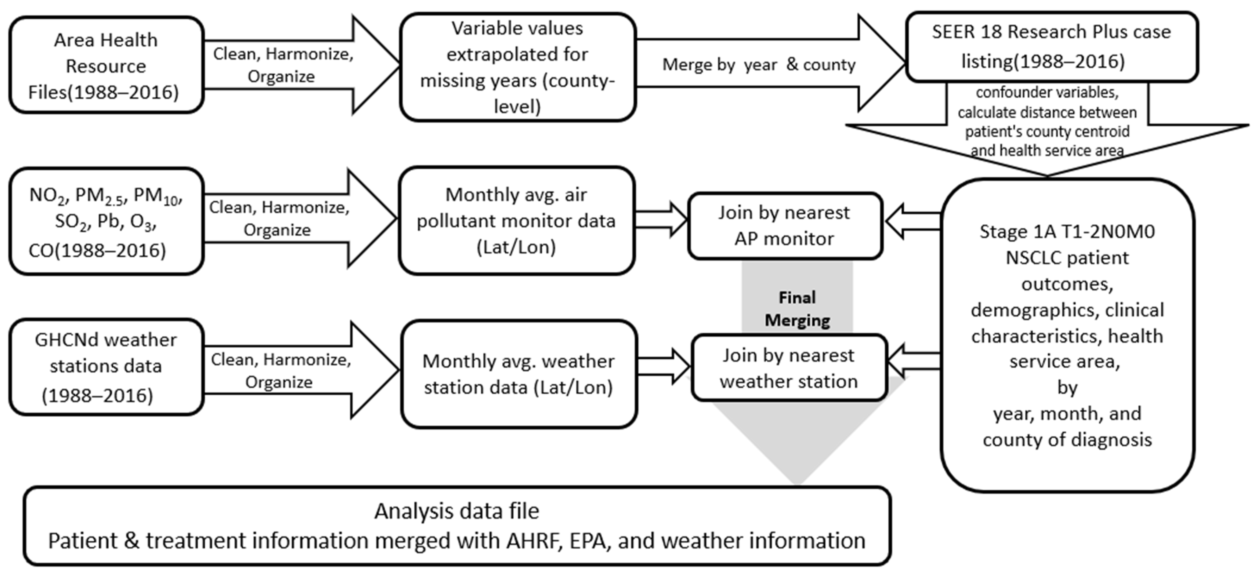
2.2. Data Sources and Construction of the Analysis Data File
2.3. Methodological Framework
2.4. Sensitivity Analyses
2.5. Ethical Considerations
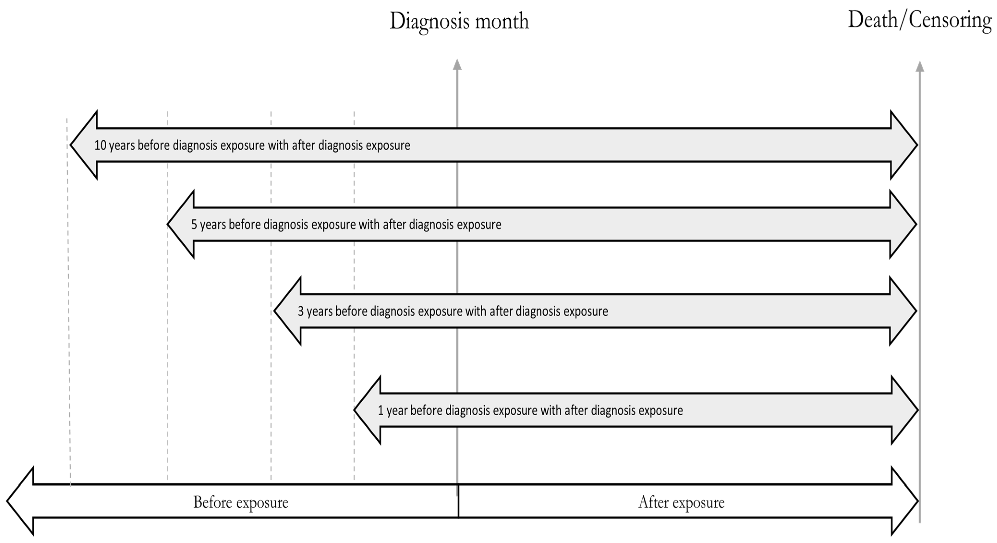
2.6. Sampling Strategy, Exposure Assignment, and Study Variables
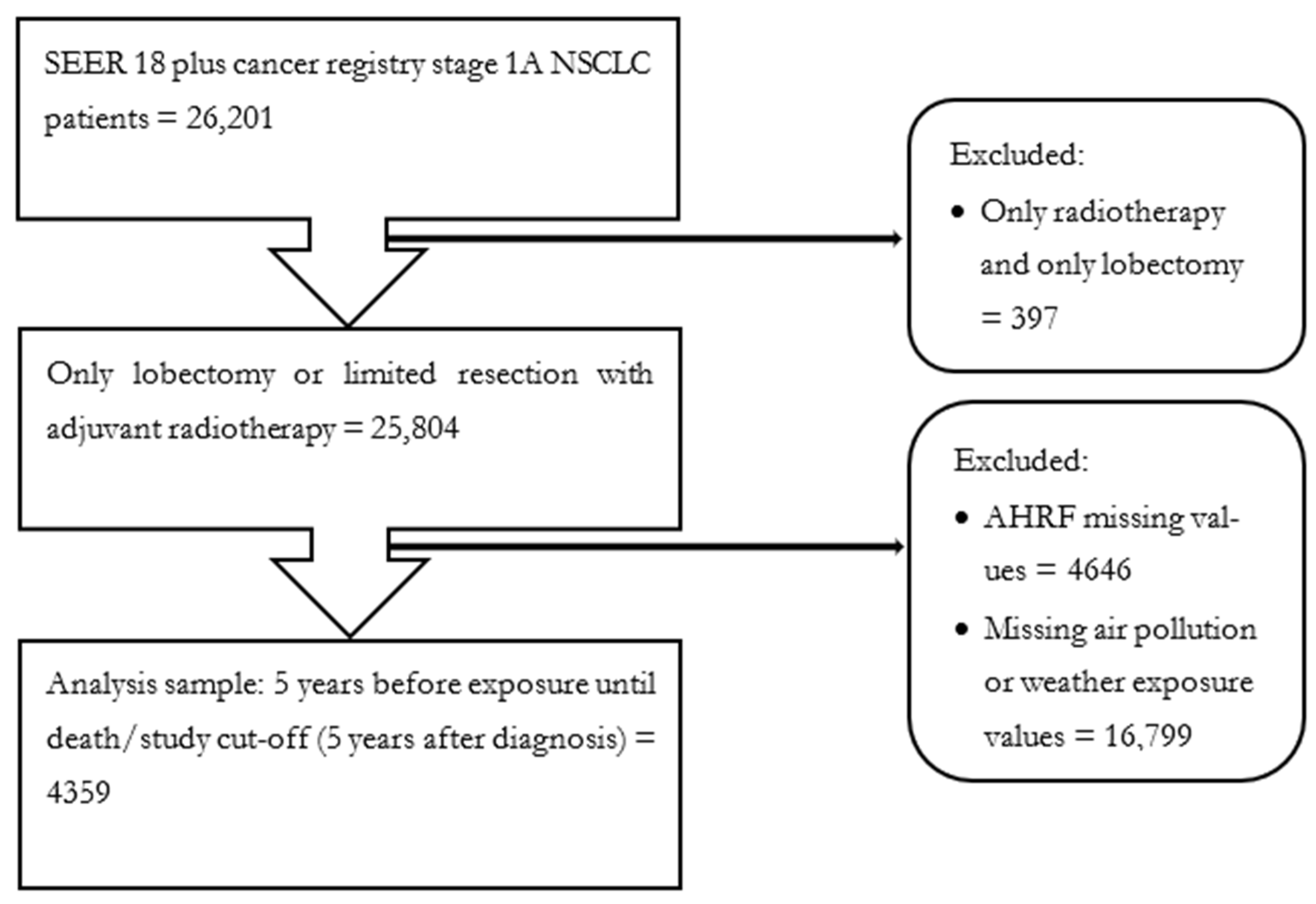
2.6.1. Population and Sample
2.6.2. Exposure Assignment
2.6.3. Independent Variables
2.6.4. Outcome Variable
2.6.5. Covariates
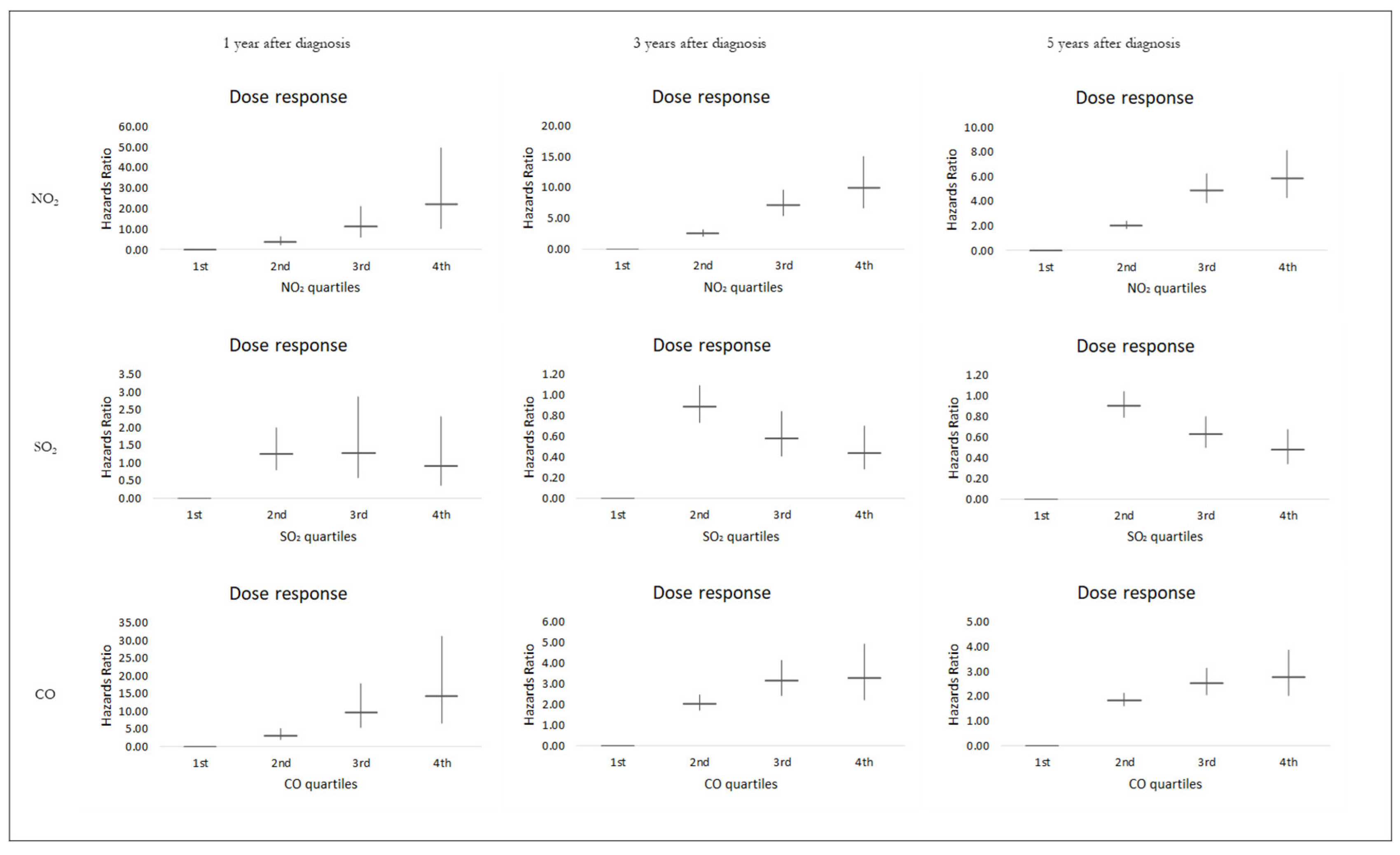
3. Results
4. Discussion
5. Implications for Practice and Policy
Author Contributions
Funding
Institutional Review Board Statement
Informed Consent Statement
Data Availability Statement
Acknowledgments
Conflicts of Interest
Appendix A

| (a) | ||||
| N | 28,509 | |||
| Frequency | Percentage | |||
| Tumor Grade | ||||
| Grade I | 6077 | 21.32 | ||
| Grade II | 10,769 | 37.77 | ||
| Grade III | 7917 | 27.77 | ||
| Grade IV | 152 | 0.53 | ||
| Unknown | 3594 | 12.61 | ||
| Tumor Size | ||||
| Up to 1 cm | 3135 | 11 | ||
| >1 cm and ≤2 cm | 8501 | 29.82 | ||
| >2 cm | 6359 | 22.31 | ||
| Unknown size | 10,514 | 36.88 | ||
| Rural Urban Continuum | ||||
| Large central metro | 7975 | 27.97 | ||
| Large fringe metro | 7403 | 25.97 | ||
| Medium metro | 6442 | 22.6 | ||
| Non-metropolitan | 6689 | 23.46 | ||
| Insurance Type | ||||
| Only Medicaid | 2913 | 10.22 | ||
| Only Medicare | 8021 | 28.13 | ||
| Only Private | 3330 | 11.68 | ||
| Uninsured | 169 | 0.59 | ||
| Unknown | 14,076 | 49.37 | ||
| Race | ||||
| Black | 4133 | 14.5 | ||
| White | 20,755 | 72.8 | ||
| Unknown | 3621 | 12.7 | ||
| Sex | ||||
| Female | 15,127 | 53.06 | ||
| Male | 13,382 | 46.94 | ||
| Marital Status | ||||
| Married | 14,404 | 50.52 | ||
| Widowed | 4807 | 16.86 | ||
| Divorced | 4483 | 15.72 | ||
| Single | 2053 | 7.2 | ||
| Unknown | 2762 | 9.69 | ||
| Treatment Guideline Revision Years | ||||
| pre 1996 | 4065 | 14.26 | ||
| post 1996 | 8475 | 29.73 | ||
| post 2005 | 625 | 2.19 | ||
| post 2006 | 768 | 2.69 | ||
| post 2007 | 6298 | 22.09 | ||
| post 2010 | 2473 | 8.67 | ||
| post 2012 | 1142 | 4.01 | ||
| post 2013 | 2662 | 9.34 | ||
| post 2015 | 2000 | 7.02 | ||
| (b) | ||||
| N | 28,509 | |||
| Median | Mean | SD | ||
| Survival months | 55 | 71.2 | 20.17 | |
| Age at diagnosis | 66 | 65.15 | 9.62 | |
| (c) | ||||
| Element monitor | Distance in miles | |||
| 25th Percentile | Median | 75th Percentile | ||
| Panel A: Sub-sample | ||||
| CO | 5.57 | 8.85 | 12.72 | |
| NO2 | 6.56 | 11.66 | 13.61 | |
| SO2 | 8.80 | 15.92 | 22.22 | |
| Precipitation | 3.34 | 3.47 | 5.40 | |
| Snow | 3.46 | 3.757 | 5.64 | |
| Daily minimum temperature | 3.37 | 5.07 | 7.05 | |
| Panel B: Above median | ||||
| CO | 5.57 | 10.43 | 11.48 | |
| NO2 | 6.56 | 11.66 | 11.77 | |
| SO2 | 8.80 | 15.31 | 15.92 | |
| Precipitation | 3.34 | 3.45 | 4.22 | |
| Snow | 3.46 | 3.55 | 5.23 | |
| Daily minimum temperature | 3.50 | 6.20 | 7.05 | |
| Panel C: Below median | ||||
| CO | 6.85 | 8.85 | 17.20 | |
| NO2 | 6.56 | 11.15 | 15.13 | |
| SO2 | 11.35 | 16.60 | 22.92 | |
| Precipitation | 2.53 | 3.58 | 6.61 | |
| Snow | 2.60 | 3.95 | 6.54 | |
| Daily minimum temperature | 2.54 | 4.19 | 6.93 | |
| (d) | ||||
| Steps | Description | |||
| 1 | (1) Rename, and clean raw files by generating date, day, year and month variables. (2) Keeping only one sample duration, and observations with non-zero latitude and longitude values (3) Generating unique siteID’s by grouping corresponding latitude and longitude (4) Generating a variable for site monitors which allots unique site monitor, a unique day number for poc numbers (5) Generating a variable for site monitors which allots same number to different poc’s per unique siteID with same day observation (6) Excluding observations with excluded even type (7) For a unique siteID only one observation is present as we keep only one poc per unique siteID | |||
| 2 | (1) Renaming and cleaning pollutant/weather data files to prep for merging (2) Assigning 3 nearest pollutant station monitor to the county centroid (3) Merging 1-3 nearest site values into one file | |||
| 3 | (1) Drop weather and AHRF variables (2) Generate 10-40 miles stations from country centroid with corresponding arithmetic mean pollutant values (3) Generating monthly values from daily values. Calculating percentage missing, for each mile: 50% , 33.33%, 25%, and 20% (4) For each mile and each % missing four monthly measures are calculated: mean, median, max and iqr (5) Collapsing all miles, all % missing, and all measures to assign corresponding only one value per month per FIPS | |||
| 4 | Appending all years, all pollutants files into one and assigning | |||
| 5 | Merging Air pollution with Weather files | |||
| 6 | After renaming variables the file is reshaped into wide format from long to achieve only one FIPS per row. The Air pollutant variables are separated from merged file to generate reshaped file and save separately for each pollutant each mile, each element, each %. | |||
| Multipollutant | NO2 | SO2 | CO | |||||||||
|---|---|---|---|---|---|---|---|---|---|---|---|---|
| Mortality Five Years Exposure Levels at Measured Timepoints Pre-/Post-Diagnosis | ||||||||||||
| 1 yr bf | 3 yrs bf | 5 yrs bf | 1 yr bf | 3 yrs bf | 5 yrs bf | 1 yr bf | 3 yrs bf | 5 yrs bf | 1 yr bf | 3 yrs bf | 5 yrs bf | |
| Air pollutants and weather elements | ||||||||||||
| NO2 | 1.04 *** | 1.05 *** | 1.08 *** | 1.05 *** | 1.07 *** | 1.10 *** | ||||||
| (1.02, 1.06) | (1.03, 1.08) | (1.06, 1.11) | (1.03, 1.62) | (1.05, 1.81) | (1.08, 8.09) | |||||||
| SO2 | 1.18 *** | 1.19 *** | 1.19 *** | 1.17 *** | 1.18 *** | 1.17 *** | ||||||
| (1.12, 1.23) | (1.14, 1.24) | (1.14, 1.24) | (1.12, 1.23) | (1.13, 1.23) | (1.12, 1.22) | |||||||
| CO | 1.39 *** | 1.41 *** | 1.52 *** | 1.73 *** | 1.89 *** | 2.27 *** | ||||||
| (1.09, 1.78) | (1.10, 1.81) | (1.17, 1.96) | (1.39, 2.14) | (1.51, 2.36) | (1.81, 2.85) | |||||||
| Precipitation | 1.01 | 1 | 1.08 | 0.96 | 0.93 | 0.98 | 1.02 | 1.02 | 1.09 * | 0.97 | 0.93 | 0.98 |
| (0.94, 1.09) | (0.91, 1.10) | (0.97, 1.20) | (0.89, 1.04) | (0.84, 1.03) | (0.89, 1.09) | (0.95, 1.10) | (0.93, 1.12) | (0.99, 1.21) | (0.90, 1.04) | (0.84, 1.02) | (0.89, 1.09) | |
| Snow | 0.76 | 0.28 | 0.05 *** | 0.45 | 0.29 | 0.09 *** | 1.24 | 0.80 | 0.44 | 1.02 | 0.38 | 0.09 *** |
| (0.16, 3.64) | (0.06, 1.34) | (0.01, 0.33) | (0.10, 1.94) | (0.06, 1.30) | (0.02, 0.50) | (0.30, 5.07) | (0.18, 3.60) | (0.08, 2.31) | (0.24, 4.31) | (0.08, 1.80) | (0.02, 0.54) | |
| Daily temperature minimum | 1.01 | 1.01 ** | 1.03 *** | 1.01 | 1.01 ** | 1.03 *** | 0.99 ** | 0.99 *** | 0.99 * | 1 | 1.01 | 1.02 *** |
| (1.00, 1.02) | (1.00, 1.02) | (1.02, 1.04) | (1.00, 1.02) | (1.00, 1.02) | (1.02, 1.04) | (0.98, 1.00) | (0.98, 0.99) | (0.98, 1.00) | (1.00, 1.01) | (1.00, 1.02) | (1.01, 1.03) | |
| Treatment options (reference: lobectomy) | ||||||||||||
| Limited resection with adjuvant radiotherapy | 1.01 | 0.99 | 1.01 | 0.74 | 0.71 | 0.75 | 1.36 | 1.32 | 1.25 | 0.99 | 0.85 | 0.84 |
| (0.64, 1.59) | (0.62, 1.59) | (0.62, 1.64) | (0.49, 1.13) | (0.47, 1.09) | (0.49, 1.13) | (0.89, 2.07) | (0.85, 2.06) | (0.79, 1.98) | (0.60, 1.36) | (0.57, 1.28) | (0.56, 1.26) | |
| Treatment interaction with air pollutant and weather elements | ||||||||||||
| NO2 × Treatment | 1.02 | 1.02 ** | 1.02 * | 1.02 *** | 1.02 *** | 1.01 *** | ||||||
| (1.00, 1.04) | (1.00, 1.04) | (1.00, 1.03) | (1.01, 1.03) | (1.01, 1.03) | (1.01, 1.02) | |||||||
| SO2 × Treatment | 0.95 | 0.95 | 0.96 | 0.98 | 0.98 | 0.98 | ||||||
| (0.88, 1.02) | (0.89, 1.02) | (0.90, 1.03) | (0.91, 1.05) | (0.91, 1.05) | (0.92, 1.05) | |||||||
| CO × Treatment | 0.99 | 1.01 | 1.01 | 1.32 *** | 1.31 *** | 1.29 *** | ||||||
| (0.70, 1.41) | (0.71, 1.44) | (0.71, 1.43) | (1.07, 1.63) | (1.07, 1.61) | (1.07, 1.56) | |||||||
| Precipitation × Treatment | 0.93 | 0.94 | 0.94 | 0.92 | 0.93 | 0.93 | 0.94 | 0.94 | 0.95 | 0.91 | 0.93 | 0.92 |
| (0.81, 1.07) | (0.84, 1.05) | (0.84, 1.05) | (0.80, 1.06) | (0.83, 1.04) | (0.83, 1.04) | (0.82, 1.07) | (0.84, 1.05) | (0.85, 1.06) | (0.79, 1.05) | (0.83, 1.03) | (0.82, 1.03) | |
| Snow × Treatment | 0.84 | 1.04 | 1.03 | 1.12 | 1.32 | 1.27 | 0.64 | 0.65 | 0.67 | 1.11 | 1.34 | 1.51 |
| (0.15, 4.76) | (0.18, 5.89) | (0.15, 6.96) | (0.20, 6.26) | (0.22, 8.02) | (0.18, 9.03) | (0.12, 3.50) | (0.12, 3.55) | (0.10, 4.23) | (0.21, 5.84) | (0.24, 7.60) | (0.23, 9.93) | |
| Temperature minimum × Treatment | 1 | 1 | 1 | 1 | 1 | 1 | 1 | 1 | 1 | 1 | 1 | 1 |
| (0.99, 1.00) | (0.99, 1.00) | (0.99, 1.00) | (1.00, 1.00) | (1.00, 1.00) | (1.00, 1.01) | (0.99, 1.00) | (0.99, 1.00) | (0.99, 1.00) | (0.99, 1.00) | (1.00, 1.00) | (1.00, 1.01) | |
| Multipollutant | NO2 | SO2 | CO | |||||||||
|---|---|---|---|---|---|---|---|---|---|---|---|---|
| Mortality Five Years Exposure Levels at Measured Timepoints Pre-/Post-Diagnosis | ||||||||||||
| 1 yr bf | 3 yrs bf | 5 yrs bf | 1 yr bf | 3 yrs bf | 5 yrs bf | 1 yr bf | 3 yrs bf | 5 yrs bf | 1 yr bf | 3 yrs bf | 5 yrs bf | |
| Air pollutants and weather elements | ||||||||||||
| NO2 | 1.02 *** | 1.02 *** | 1.02 *** | 1.04 *** | 1.05 *** | 1.05 *** | ||||||
| (1.01, 1.04) | (1.01, 1.04) | (1.01, 1.04) | (1.03, 1.50) | (1.04, 1.72) | (1.04, 2.35) | |||||||
| SO2 | 1.04 *** | 1.04 *** | 1.04 *** | 1.04 *** | 1.04 *** | 1.04 *** | ||||||
| (1.02, 1.05) | (1.02, 1.05) | (1.03, 1.05) | (1.02, 1.05) | (1.03, 1.05) | (1.03, 1.05) | |||||||
| CO | 1.55 *** | 1.61 *** | 1.64 *** | 1.79 *** | 1.97 *** | 2.05 *** | ||||||
| (1.34, 1.79) | (1.36, 1.90) | (1.36, 1.98) | 1 *** | 1 *** | 1 * | (1.58, 2.04) | (1.72, 2.24) | (1.80, 2.33) | ||||
| Precipitation | 1 *** | 1 *** | 1 *** | (1, 1) | (1, 1) | (1, 1) | 1.00 | 1.00 | 1.00 | 1 *** | 1 *** | 1 *** |
| (1, 1) | (1, 1) | (1, 1) | 1.00 | 0.99 ** | 0.99 ** | (1, 1) | (1, 1) | (1, 1) | (1, 1) | (1, 1) | (1, 1) | |
| Snow | 1.00 | 0.99 ** | 0.99 ** | (0.99, 1.00) | (0.99, 1.00) | (0.98, 1.00) | 1.00 | 1.00 | 0.99 | 1.00 | 0.99 | 0.99 ** |
| (0.99, 1.00) | (0.99, 1.00) | (0.98, 1.00) | 1.01 *** | 1.01 *** | 1.02 *** | (0.99, 1.01) | (0.99, 1.01) | (0.99, 1.00) | (0.99, 1.00) | (0.99, 1.00) | (0.98, 1.00) | |
| Daily temperature minimum | 1.01 *** | 1.01 *** | 1.02 *** | (1.00, 1.01) | (1.00, 1.02) | (1.01, 1.03) | 1.00 | 1.00 | 1.01 | 1.01 *** | 1.01 *** | 1.02 *** |
| (1.00, 1.02) | (1.01, 1.02) | (1.01, 1.03) | 1 *** | 1 *** | 1 * | (0.99, 1.00) | (0.99, 1.01) | (1.00, 1.02) | (1.00, 1.02) | (1.01, 1.02) | (1.01, 1.03) | |
| Treatment options (reference: lobectomy) | ||||||||||||
| Limited resection with adjuvant radiotherapy | 1.40 | 1.07 | 1.11 | 0.94 | 0.73 | 0.76 | 1.69 | 1.08 | 0.89 | 1.14 | 0.85 | 0.77 |
| (0.50, 3.88) | (0.35, 3.26) | (0.35, 3.51) | (0.36, 2.43) | (0.27, 2.00) | (0.28, 2.10) | (0.57, 5.04) | (0.35, 3.31) | (0.29, 2.75) | (0.42, 3.10) | (0.30, 2.38) | (0.28, 2.16) | |
| Treatment interaction with air pollutant and weather elements | ||||||||||||
| NO2 × Treatment | 1.02 | 1.02 *** | 1.02 *** | 1.01 *** | 1.01 *** | 1.01 *** | ||||||
| (1.01, 1.04) | (1.01, 1.04) | (1.01, 1.03) | (1.01, 1.02) | (1.01, 1.02) | (1.01, 1.02) | |||||||
| SO2 × Treatment | 0.99 | 0.99 | 0.99 | 1 | 1 | 1 | ||||||
| (0.97, 1.00) | (0.97, 1.01) | (0.97, 1.01) | (0.98, 1.01) | (0.98, 1.02) | (0.99, 1.02) | |||||||
| CO × Treatment | 0.85 | 0.85 | 0.86 | 1.16 ** | 1.16 ** | 1.15 *** | ||||||
| (0.68, 1.07) | (0.69, 1.06) | (0.69, 1.06) | (1.03, 1.32) | (1.03, 1.30) | (1.03, 1.28) | |||||||
| Precipitation × Treatment | 1 | 1 | 1 | 1 | 1 | 1 | 1 | 1 | 1 | 1 | 1 | 1 |
| (1, 1) | (1, 1) | (1, 1) | (1, 1) | (1, 1) | (1, 1) | (1, 1) | (1, 1) | (1, 1) | (1, 1) | (1, 1) | (1, 1) | |
| Snow × Treatment | 1 | 1 | 1 | 1 | 1 | 1 | 1 | 1 | 1 | 1 | 1 | 1 |
| (0.99, 1.00) | (0.99, 1.00) | (0.99, 1.00) | (0.99, 1.00) | (0.99, 1.00) | (0.99, 1.00) | (0.99, 1.00) | (0.99, 1.00) | (0.99, 1.00) | (0.99, 1.01) | (0.99, 1.01) | (0.99, 1.01) | |
| Temperature minimum × Treatment | 0.99* | 0.99 | 0.99 | 1 | 1 | 1 | 0.99 | 1 | 1 | 1 | 1 | 1 |
| (0.98, 1.00) | (0.99, 1.00) | (0.98, 1.00) | (0.99, 1.00) | (0.99, 1.01) | (0.99, 1.01) | (0.99, 1.00) | (0.99, 1.01) | (0.99, 1.01) | (0.99, 1.00) | (0.99, 1.01) | (0.99, 1.01) | |
| Multipollutant | NO2 | SO2 | CO | |||||
|---|---|---|---|---|---|---|---|---|
| Mortality Five Years Exposure Levels at Measured Timepoints Pre-/Post-Diagnosis | ||||||||
| 1 yr bf | 3 yrs. bf | 1 yr bf | 3 yrs. bf | 1 yr bf | 3 yrs. bf | 1 yr bf | 3 yrs. bf | |
| Air pollutants and weather components | ||||||||
| NO2 | 1.04 *** | 1.06 *** | 1.06 *** | 1.08 *** | ||||
| (1.02, 1.06) | (1.04, 1.08) | (1.04, 1.29) | (1.06, 1.68) | |||||
| SO2 | 1.16 *** | 1.17 *** | 1.15 *** | 1.16 *** | ||||
| (1.12, 1.21) | (1.13, 1.22) | (1.11, 1.20) | (1.12, 1.21) | |||||
| CO | 1.53 *** | 1.51 *** | 1.90 *** | 2.07 *** | ||||
| (1.19, 1.97) | (1.16, 1.96) | (1.52, 2.38) | (1.65, 2.60) | |||||
| Precipitation | 0.98 ** | 0.97 *** | 0.98 ** | 0.98 *** | 1 | 1 | 0.99 * | 0.98 ** |
| (0.97, 1) | (0.95, 0.99) | (0.97, 1) | (0.96, 0.99) | (0.98, 1.01) | (0.98, 1.01) | (0.97, 1) | (0.96, 1) | |
| Snow | 0.99 | 0.96 | 0.94 | 0.88 *** | 1 | 1.01 | 1 | 0.94 |
| (0.92, 1.07) | (0.88, 1.05) | (0.87, 1.01) | (0.81, 0.96) | (0.93, 1.08) | (0.93, 1.10) | (0.93, 1.07) | (0.87, 1.03) | |
| Daily temperature minimum | 1.01 | 1.01 ** | 1.01 | 1.01 ** | 0.99 ** | 0.99 ** | 1.01 | 1.01 |
| (1, 1.02) | (1, 1.02) | (1, 1.01) | (1, 1.02) | (0.99, 1) | (0.98, 1) | (1, 1.01) | (1, 1.02) | |
| Treatment options (reference: lobectomy) | ||||||||
| Daily temperature minimum | 1.01 | 1.01 ** | 1.01 | 1.01 ** | 0.99 ** | 0.99 ** | 1.01 | 1.01 |
| (1, 1.02) | (1, 1.02) | (1, 1.01) | (1, 1.02) | (0.99, 1) | (0.98, 1) | (1, 1.01) | (1, 1.02) | |
| Treatment interaction with air pollutants and weather components | ||||||||
| NO2 × Treatment | 1.01 | 1.02 * | 1.01 * | 1.01 * | ||||
| (1, 1.03) | (1, 1.03) | (1, 1.02) | (1, 1.02) | |||||
| SO2 × Treatment | 0.99 | 0.98 | 1.02 | 1.02 | ||||
| (0.93, 1.04) | (0.93, 1.04) | (0.97, 1.07) | (0.98, 1.07) | |||||
| CO × Treatment | 0.94 | 0.85 | 1.16 | 1.24 ** | ||||
| (0.68, 1.29) | (0.60, 1.21) | (0.95, 1.43) | (1.04, 1.48) | |||||
| Precipitation × Treatment | 1 | 1.01 | 1 | 1 | 1 | 1.01 * | 1 | 1 |
| (0.99, 1.01) | (1, 1.02) | (0.99, 1) | (0.99, 1.01) | (1, 1.01) | (1, 1.02) | (0.99, 1.01) | (0.99, 1.01) | |
| Snow × Treatment | 1.10 ** | 1.14 *** | 1.03 | 1.04 | 1.09 ** | 1.10 ** | 1.03 | 1.06 |
| (1, 1.20) | (1.03, 1.25) | (0.96, 1.10) | (0.97, 1.12) | (1, 1.18) | (1, 1.20) | (0.95, 1.12) | (0.98, 1.14) | |
| Temperature minimum × Treatment | 1 | 1.01 * | 1 | 1 | 1.01 ** | 1.01 ** | 1 | 1 |
| (1, 1.01) | (1, 1.02) | (1, 1.01) | (1, 1.01) | (1, 1.01) | (1, 1.01) | (1, 1.01) | (1, 1.01) | |
| Race (reference: Black) | ||||||||
| Other | 1 | 1 | 1.02 | 1.02 | 0.99 | 0.98 | 1.02 | 1.01 |
| (0.87, 1.16) | (0.86, 1.15) | (0.88, 1.18) | (0.88, 1.18) | (0.86, 1.14) | (0.85, 1.13) | (0.88, 1.17) | (0.88, 1.17) | |
| White | 0.97 | 0.96 | 0.98 | 0.98 | 0.96 | 0.95 | 0.97 | 0.97 |
| (0.88, 1.07) | (0.88, 1.06) | (0.89, 1.08) | (0.89, 1.08) | (0.87, 1.06) | (0.87, 1.05) | (0.88, 1.07) | (0.88, 1.07) | |
| Sex (reference: Female) | ||||||||
| Male | 1.12 *** | 1.12 *** | 1.12 *** | 1.12 *** | 1.11 *** | 1.11 *** | 1.12 *** | 1.12 *** |
| (1.05, 1.19) | (1.05, 1.19) | (1.05, 1.19) | (1.06, 1.19) | (1.04, 1.17) | (1.04, 1.18) | (1.05, 1.19) | (1.05, 1.19) | |
| Tumor Grade (reference: II) | ||||||||
| Grade III | 1.10 *** | 1.10 *** | 1.09 ** | 1.09 ** | 1.12 *** | 1.12 *** | 1.09 ** | 1.09 ** |
| (1.02, 1.19) | (1.02, 1.19) | (1.01, 1.18) | (1.01, 1.17) | (1.04, 1.20) | (1.04, 1.20) | (1.01, 1.18) | (1.02, 1.18) | |
| Grade IV | 1 | 0.99 | 0.98 | 0.97 | 1.01 | 1.01 | 0.96 | 0.95 |
| (0.72, 1.39) | (0.71, 1.37) | (0.70, 1.38) | (0.69, 1.36) | (0.72, 1.41) | (0.72, 1.42) | (0.68, 1.37) | (0.67, 1.35) | |
| Unknown | 0.95 | 0.94 | 0.95 | 0.95 | 0.94 | 0.94 | 0.94 | 0.94 |
| (0.85, 1.06) | (0.85, 1.05) | (0.85, 1.06) | (0.85, 1.06) | (0.84, 1.05) | (0.84, 1.05) | (0.85, 1.05) | (0.84, 1.05) | |
| Grade I | 0.92 ** | 0.92 ** | 0.93 * | 0.93 * | 0.92 ** | 0.93 ** | 0.93 * | 0.93 * |
| (0.85, 1) | (0.86, 1) | (0.86, 1) | (0.86, 1) | (0.86, 1) | (0.86, 1) | (0.86, 1) | (0.86, 1) | |
| Marital status (reference: Divorced) | ||||||||
| Married | 0.96 | 0.96 | 0.96 | 0.96 | 0.95 | 0.95 | 0.96 | 0.96 |
| (0.88, 1.05) | (0.88, 1.06) | (0.88, 1.05) | (0.88, 1.06) | (0.86, 1.04) | (0.86, 1.04) | (0.88, 1.05) | (0.88, 1.06) | |
| Single | 0.98 | 0.98 | 0.98 | 0.98 | 0.96 | 0.95 | 0.96 | 0.97 |
| (0.87, 1.10) | (0.87, 1.10) | (0.87, 1.10) | (0.87, 1.11) | (0.85, 1.08) | (0.85, 1.07) | (0.85, 1.08) | (0.86, 1.09) | |
| Unknown | 0.98 | 0.99 | 0.99 | 1 | 0.98 | 0.98 | 0.97 | 0.98 |
| (0.84, 1.15) | (0.85, 1.16) | (0.84, 1.16) | (0.85, 1.16) | (0.84, 1.15) | (0.83, 1.15) | (0.83, 1.14) | (0.84, 1.14) | |
| Widowed | 0.98 | 0.98 | 0.98 | 0.99 | 0.96 | 0.96 | 0.97 | 0.98 |
| (0.87, 1.10) | (0.88, 1.11) | (0.88, 1.11) | (0.88, 1.11) | (0.85, 1.08) | (0.85, 1.08) | (0.87, 1.09) | (0.87, 1.10) | |
| Tumor size (reference: up to 1 cm) | ||||||||
| >1 cm & ≤2 cm | 0.99 | 0.99 | 1 | 1 | 0.99 | 0.99 | 1.01 | 1.01 |
| (0.89, 1.10) | (0.89, 1.10) | (0.90, 1.11) | (0.90, 1.11) | (0.90, 1.10) | (0.89, 1.09) | (0.91, 1.12) | (0.91, 1.12) | |
| >2 cm | 1.02 | 1.02 | 1.02 | 1.02 | 1.02 | 1.01 | 1.03 | 1.02 |
| (0.91, 1.14) | (0.91, 1.14) | (0.91, 1.14) | (0.91, 1.14) | (0.91, 1.14) | (0.91, 1.13) | (0.92, 1.15) | (0.92, 1.15) | |
| Unknown | 0.87 | 0.85 | 0.88 | 0.86 | 0.84 | 0.82 | 0.76 | 0.75 |
| (0.49, 1.55) | (0.47, 1.57) | (0.49, 1.56) | (0.47, 1.57) | (0.48, 1.47) | (0.47, 1.44) | (0.42, 1.38) | (0.41, 1.39) | |
| Tumor histology (reference: squamous cell) | ||||||||
| Adenomas | 0.94 | 0.95 | 0.94 * | 0.94 | 0.94 * | 0.94 | 0.93 * | 0.93 * |
| (0.87, 1.01) | (0.88, 1.02) | (0.87, 1.01) | (0.87, 1.01) | (0.87, 1.01) | (0.87, 1.01) | (0.87, 1.01) | (0.87, 1.01) | |
| Age at diagnosis | 1.01 *** | 1.01 *** | 1.01 *** | 1.01 *** | 1.01 *** | 1.01 *** | 1.01 *** | 1.01 *** |
| (1, 1.01) | (1, 1.01) | (1, 1.01) | (1, 1.01) | (1, 1.01) | (1, 1.01) | (1, 1.01) | (1, 1.01) | |
| Insurance type (reference: Only Medicaid) | ||||||||
| Only Medicare | 0.93 | 0.93 | 0.94 | 0.94 | 0.94 | 0.94 | 0.92 | 0.92 |
| (0.81, 1.07) | (0.81, 1.08) | (0.82, 1.08) | (0.82, 1.08) | (0.82, 1.09) | (0.82, 1.09) | (0.80, 1.06) | (0.79, 1.06) | |
| Only private | 0.97 | 0.97 | 0.97 | 0.96 | 1 | 0.99 | 0.95 | 0.94 |
| (0.84, 1.12) | (0.84, 1.12) | (0.84, 1.11) | (0.84, 1.11) | (0.87, 1.15) | (0.86, 1.14) | (0.82, 1.09) | (0.82, 1.09) | |
| Uninsured | 1.27 | 1.31 * | 1.17 | 1.19 | 1.22 | 1.23 | 1.15 | 1.17 |
| (0.92, 1.76) | (0.95, 1.81) | (0.85, 1.61) | (0.87, 1.64) | (0.89, 1.68) | (0.90, 1.69) | (0.83, 1.58) | (0.86, 1.61) | |
| Unknown | 1.05 | 1.07 | 0.93 | 0.96 | 1.07 | 1.09 | 0.98 | 0.98 |
| (0.80, 1.37) | (0.82, 1.40) | (0.71, 1.21) | (0.73, 1.25) | (0.83, 1.39) | (0.84, 1.41) | (0.74, 1.28) | (0.75, 1.29) | |
| Rural-Urban continuum (reference: Large central metro) | ||||||||
| Large fringe metro | 0.84 | 0.93 | 0.98 | 1.16 | 0.57 | 0.55 | 0.86 | 0.91 |
| (0.26, 2.67) | (0.28, 3.12) | (0.34, 2.84) | (0.40, 3.38) | (0.19, 1.72) | (0.18, 1.66) | (0.29, 2.58) | (0.30, 2.80) | |
| Medium metro | 0.10 *** | 0.07 *** | 0.11 *** | 0.10 *** | 0.16 *** | 0.15 *** | 0.12 *** | 0.12 *** |
| (0.04, 0.27) | (0.03, 0.20) | (0.04, 0.30) | (0.03, 0.28) | (0.06, 0.40) | (0.06, 0.40) | (0.05, 0.31) | (0.05, 0.34) | |
| Non-metropolitan | 0.45 * | 0.46 | 0.53 | 0.64 | 0.23 *** | 0.24 *** | 0.37 ** | 0.36 ** |
| (0.18, 1.10) | (0.17, 1.21) | (0.21, 1.29) | (0.24, 1.68) | (0.10, 0.56) | (0.09, 0.61) | (0.15, 0.87) | (0.14, 0.91) | |
References
- Strickland, M.J.; Gass, K.M.; Goldman, G.T.; Mulholland, J.A. Effects of ambient air pollution measurement error on health effect estimates in time-series studies: A simulation-based analysis. J. Expo. Sci. Environ. Epidemiol. 2015, 25, 160–166. [Google Scholar] [CrossRef] [PubMed]
- Baxter, L.K.; Dionisio, K.L.; Burke, J.; Ebelt Sarnat, S.; Sarnat, J.A.; Hodas, N.; Rich, D.Q.; Turpin, B.J.; Jones, R.R.; Mannshardt, E.; et al. Exposure prediction approaches used in air pollution epidemiology studies: Key findings and future recommendations. J. Expo. Sci. Environ. Epidemiol. 2013, 23, 654–659. [Google Scholar] [CrossRef]
- Eckel, S.P.; Cockburn, M.; Shu, Y.H.; Deng, H.; Lurmann, F.W.; Liu, L.; Gilliland, F.D. Air pollution affects lung cancer survival. Thorax 2016, 71, 891–898. [Google Scholar] [CrossRef] [PubMed]
- Aksoy, M. Different types of malignancies due to occupational exposure to benzene: A review of recent observations in Turkey. Environ. Res. 1980, 23, 181–190. [Google Scholar] [CrossRef] [PubMed]
- McKeon, T.P.; Vachani, A.; Penning, T.M.; Hwang, W.T. Air pollution and lung cancer survival in Pennsylvania. Lung Cancer 2022, 170, 65. [Google Scholar] [CrossRef]
- Pyo, J.S.; Kim, N.Y.; Kang, D.W. Impacts of Outdoor Particulate Matter Exposure on the Incidence of Lung Cancer and Mortality. Medicina 2022, 58, 1159. [Google Scholar] [CrossRef]
- Liu, C.S.; Wei, Y.; Danesh Yazdi, M.; Qiu, X.; Castro, E.; Zhu, Q.; Li, L.; Koutrakis, P.; Ekenga, C.C.; Shi, L.; et al. Long-term association of air pollution and incidence of lung cancer among older Americans: A national study in the Medicare cohort. Environ. Int. 2023, 181, 108266. [Google Scholar] [CrossRef]
- Lee, H.C.; Lu, Y.H.; Huang, Y.L.; Huang, S.L.; Chuang, H.C. Air Pollution Effects to the Subtype and Severity of Lung Cancers. Front. Med. 2022, 9, 835026. [Google Scholar] [CrossRef]
- Lamichhane, D.K.; Kim, H.; Choi, C.; Shin, M.; Shim, Y.M.; Leem, J.; Ryu, J.; Nam, H.; Park, S. Lung Cancer Risk and Residential Exposure to Air Pollution: A Korean Population-Based Case-Control Study. Yonsei Med. J. 2017, 58, 1111–1118. [Google Scholar] [CrossRef]
- Moon, D.H.; Kwon, S.O.; Kim, S.Y.; Kim, W.J. Air Pollution and Incidence of Lung Cancer by Histological Type in Korean Adults: A Korean National Health Insurance Service Health Examinee Cohort Study. Int. J. Environ. Res. Public Health 2020, 17, 915. [Google Scholar] [CrossRef]
- Zanobetti, A.; Peters, A. Disentangling interactions between atmospheric pollution and weather. J. Epidemiol. Community Health 2015, 69, 613. [Google Scholar] [CrossRef] [PubMed]
- Tian, X.; Cui, K.; Sheu, H.L.; Hsieh, Y.K.; Yu, F. Effects of rain and snow on the air quality index, PM2.5 levels, and dry deposition flux of PCDD/Fs. Aerosol Air Qual. Res. 2021, 21, 210158. [Google Scholar] [CrossRef]
- Kim, S.Y.; Sheppard, L.; Kim, H. Health effects of long-term air pollution: Influence of exposure prediction methods. Epidemiology 2009, 20, 442–450. [Google Scholar] [CrossRef]
- Zheng, Z.; Xu, G.; Li, Q.; Chen, C.; Li, J. Effect of precipitation on reducing atmospheric pollutant over Beijing. Atmos. Pollut. Res. 2019, 10, 1443–1453. [Google Scholar] [CrossRef]
- Wang, Y.; Guo, Z.; Han, J. The relationship between urban heat island and air pollutants and them with influencing factors in the Yangtze River Delta, China. Ecol. Indic. 2021, 129, 107976. [Google Scholar] [CrossRef]
- Ngarambe, J.; Joen, S.J.; Han, C.H.; Yun, G.Y. Exploring the relationship between particulate matter, CO, SO2, NO2, O3 and urban heat island in Seoul, Korea. J. Hazard. Mater. 2021, 403, 123615. [Google Scholar] [CrossRef] [PubMed]
- De Sario, M.; Katsouyanni, K.; Michelozzi, P. Climate change, extreme weather events, air pollution and respiratory health in Europe. Eur. Respir. J. 2013, 42, 826–843. [Google Scholar] [CrossRef]
- Liu, Y.; Zhou, Y.; Lu, J. Exploring the relationship between air pollution and meteorological conditions in China under environmental governance. Sci. Rep. 2020, 10, 14518. [Google Scholar] [CrossRef]
- Oji, S.; Adamu, H. Correlation between air pollutants concentration and meteorological factors on seasonal air quality variation. J. Air Pollut. Health 2020, 5, 11–32. [Google Scholar] [CrossRef]
- Sofia, D.; Lotrecchiano, N.; Giuliano, A.; Barletta, D.; Poletto, M. Optimization of number and location of sampling points of an air quality monitoring network in an urban contest. Chem. Eng. Trans. 2019, 74, 277–282. [Google Scholar] [CrossRef]
- US EPA. Air Pollutant Receptor Modeling. United States Environmental Protection Agency. 2025. Available online: https://www.epa.gov/scram/air-pollutant-receptor-modeling (accessed on 23 April 2025).
- US EPA. Models, Tools and Databases for Air Research. United States Environmental Protection Agency. 2025. Available online: https://19january2017snapshot.epa.gov/air-research/models-tools-and-databases-air-research_.html (accessed on 23 April 2025).
- US EPA. Air Quality Models. United States Environmental Protection Agency. 2025. Available online: https://www.epa.gov/scram/air-quality-models (accessed on 23 April 2025).
- Cao, J.; Yuan, P.; Wang, Y.; Xu, J.; Yuan, X.; Wang, Z.; Lv, W.; Hu, J. Survival Rates After Lobectomy, Segmentectomy, and Wedge Resection for Non-Small Cell Lung Cancer. Ann. Thorac. Surg. 2018, 105, 1483–1491. [Google Scholar] [CrossRef] [PubMed]
- Raman, V.; Jawitz, O.K.; Cerullo, M.; Voigt, S.L.; Rhodin, K.E.; Yang, C.-F.J.; D’Amico, T.A.; Harpole, D.H.; Kelsey, C.R.; Tong, B.C. Tumor Size, Histology, and Survival After Stereotactic Ablative Radiotherapy and Sublobar Resection in Node-negative Non-small Cell Lung Cancer. Ann. Surg. 2022, 276, e1000–e1007. [Google Scholar] [CrossRef] [PubMed]
- Baig, M.Z.; Razi, S.S.; Weber, J.F.; Connery, C.P.; Bhora, F.Y. Lobectomy is superior to segmentectomy for peripheral high grade non-small cell lung cancer ≤2 cm. J. Thorac. Dis. 2020, 12, 5925–5933. [Google Scholar] [CrossRef]
- Shen, J.; Zhuang, W.; Xu, C.; Jin, K.; Chen, B.; Tian, D.; Hiley, C.; Onishi, H.; Zhu, C.; Qiao, G. Surgery or Non-surgical Treatment of ≤8 mm Non-small Cell Lung Cancer: A Population-Based Study. Front. Surg. 2021, 8, 632561. [Google Scholar] [CrossRef]
- Patel, N.; Karimi, S.; Egger, M.E.; Little, B.; Antimisiaris, D. Disparity in Treatment Receipt by Race and Treatment Guideline Revision Years for Stage 1A Non-Small Cell Lung Cancer Patients in the US. J. Racial Ethn. Health Disparities 2024, 24, 1–13. [Google Scholar] [CrossRef] [PubMed]
- Liu, C.; Yang, D.; Liu, Y.; Piao, H.; Zhang, T.; Li, X.; Zhao, E.; Zhang, D. The effect of ambient—On survival of lung cancer patients after lobectomy. Environ. Health 2023, 22, 23. [Google Scholar] [CrossRef]
- Xu, X.; Ha, S.; Kan, H.; Hu, H.; Curbow, B.A.; Lissaker, C.T. Health effects of air pollution on length of respiratory cancer survival. BMC Public Health 2013, 13, 800. [Google Scholar] [CrossRef]
- Health Resources and Services Administration. “Area Health Resources Files,” HRSA. Available online: https://data.hrsa.gov/topics/health-workforce/ahrf (accessed on 23 April 2025).
- SEER. “Overview of the SEER Program,” Surveillance, Epidemiology, and End Results Program. Available online: https://seer.cancer.gov/about/overview.html (accessed on 23 April 2025).
- Rivera-González, L.O.; Zhang, Z.; Sánchez, B.N.; Zhang, K.; Brown, D.G.; Rojas-Bracho, L.; Osornio-Vargas, A.; Vadillo-Ortega, F.; O’Neill, M.S. An Assessment of Air Pollutant Exposure Methods in Mexico City, Mexico. J. Air Waste Manag. Assoc. 1995, 65, 581. [Google Scholar] [CrossRef]
- Wei, Y.; Qiu, X.; Yazdi, M.D.; Shtein, A.; Shi, L.; Yang, J.; Peralta, A.A.; Coull, B.A.; Schwartz, J.D. The Impact of Exposure Measurement Error on the Estimated Concentration-Response Relationship between Long-Term Exposure to PM2.5 and Mortality. Environ. Health Perspect. 2022, 130, 77006. [Google Scholar] [CrossRef]
- Razi, S.S.; John, M.M.; Sainathan, S.; Stavropoulos, C. Sublobar resection is equivalent to lobectomy for T1a non-small cell lung cancer in the elderly: A Surveillance, Epidemiology, and End Results database analysis. J. Surg. Res. 2016, 200, 683–689. [Google Scholar] [CrossRef]
- Kates, M.; Swanson, S.; Wisnivesky, J.P. Survival following lobectomy and limited resection for the treatment of stage I non-small cell lung cancer ≤1 cm in size: A review of SEER data. Chest 2011, 139, 491–496. [Google Scholar] [CrossRef] [PubMed]
- Mery, C.M.; Pappas, A.N.; Bueno, R.; Colson, Y.L.; Linden, P.; Sugarbaker, D.J.; Jaklitsch, M.T. Similar long-term survival of elderly patients with non-small cell lung cancer treated with lobectomy or wedge resection within the surveillance, epidemiology, and end results database. Chest 2005, 128, 237–245. [Google Scholar] [CrossRef] [PubMed]
- Altorki, N.K.; Wang, X.; Wigle, D.; Gu, L.; Darling, G.; Ashrafi, A.S.; Landrenau, R.; Miller, D.; Jones, D.R.; Keenan, R.; et al. Perioperative mortality and Morbidity after Lobar versus Sublobar Resection for early stage lung cancer: A post-hoc analysis of an international randomized phase III trial (CALGB/ Alliance 140503). Lancet Respir. Med. 2019, 6, 915–924. [Google Scholar] [CrossRef] [PubMed]
- Rueth, N.M.; Parsons, H.M.; Habermann, E.B.; Groth, S.S.; Virnig, B.A.; Tuttle, T.M.; Andrade, R.S.; Maddaus, M.A.; D’Cunha, J. Surgical treatment of lung cancer: Predicting postoperative morbidity in the elderly population. J. Thorac. Cardiovasc. Surg. 2012, 143, 1314–1323. [Google Scholar] [CrossRef]
- Lee, K.K.; Bing, R.; Kiang, J.; Bashir, S.; Spath, N.; Stelzle, D.; Mortimer, K.; Bularga, A.; Doudesis, D.; Joshi, S.S.; et al. Adverse health effects associated with household air pollution: A systematic review, meta-analysis, and burden estimation study. Lancet Glob. Health 2020, 8, e1427–e1434. [Google Scholar] [CrossRef]


| (a) | ||||||||
| Above Median | Below Median | |||||||
| Frequency | Percentage | Frequency | Percentage | |||||
| Tumor Grade | ||||||||
| Grade I | 262 | 12.02 | 484 | 22.20 | ||||
| Grade II | 877 | 40.25 | 929 | 42.61 | ||||
| Grade III | 835 | 38.32 | 564 | 25.87 | ||||
| Grade IV | 30 | 1.38 | 16 | 0.73 | ||||
| Unknown | 175 | 8.03 | 187 | 8.58 | ||||
| Tumor size | ||||||||
| Up to 1 cm | 42 | 1.93 | 198 | 9.08 | ||||
| >1 cm and ≤2 cm | 208 | 9.55 | 820 | 37.61 | ||||
| >2 cm | 189 | 8.67 | 643 | 29.50 | ||||
| Unknown size | 1740 | 79.85 | 519 | 23.81 | ||||
| Treatment type | ||||||||
| Only lobectomy | 1951 | 89.54 | 1815 | 83.26 | ||||
| Limited resection with adjuvant | 228 | 10.46 | 365 | 16.74 | ||||
| Rural–urban continuum | ||||||||
| Large central metro | 1333 | 61.17 | 1138 | 52.20 | ||||
| Large fringe metro | 536 | 24.60 | 801 | 36.74 | ||||
| Medium metro | 285 | 13.08 | 195 | 8.94 | ||||
| Non-metropolitan | 25 | 1.15 | 46 | 2.11 | ||||
| Insurance type | ||||||||
| Only Medicaid | 35 | 1.61 | 125 | 5.73 | ||||
| Only Medicare | 166 | 7.62 | 823 | 37.75 | ||||
| Only Private | 69 | 3.17 | 468 | 21.47 | ||||
| Uninsured | 6 | 0.28 | 16 | 0.73 | ||||
| Unknown | 1903 | 87.33 | 748 | 34.31 | ||||
| Race | ||||||||
| Black | 288 | 13.22 | 228 | 10.46 | ||||
| White | 1773 | 81.37 | 1759 | 80.69 | ||||
| Unknown | 118 | 5.42 | 193 | 8.85 | ||||
| Sex | ||||||||
| Female | 969 | 44.47 | 1226 | 56.24 | ||||
| Male | 1210 | 55.53 | 954 | 43.76 | ||||
| Marital Status | ||||||||
| Married | 1280 | 58.74 | 1239 | 56.83 | ||||
| Widowed | 380 | 17.44 | 277 | 12.71 | ||||
| Divorced | 247 | 11.34 | 284 | 13.03 | ||||
| Single | 224 | 10.28 | 278 | 12.75 | ||||
| Unknown | 48 | 2.20 | 102 | 4.68 | ||||
| N | 2179 | 2180 | ||||||
| (b) | ||||||||
| Above median | Below median | |||||||
| Median | Mean | SD | Median | Mean | SD | |||
| Months of survival | 27 | 28.11 | 17.61 | 30 | 31.09 | 15.93 | ||
| Panel A: Exposure to air pollutants before and after diagnosis | ||||||||
| NO2 exposure (ppb) | 22.25 | 25.66 | 3.61 | 12.71 | 12.97 | 3.61 | ||
| SO2 exposure (ppb) | 4.10 | 3.98 | 1.20 | 1.56 | 1.81 | 1.20 | ||
| CO exposure (ppb) | 816.75 | 1010.84 | 214.13 | 371.03 | 447.91 | 214.13 | ||
| Panel B: Weather conditions before and after diagnosis | ||||||||
| Precipitation | 24.06 | 26.07 | 8.76 | 22.41 | 23.34 | 10.93 | ||
| Snow | 0.98 | 1.14 | 1.15 | 0.10 | 1.28 | 1.54 | ||
| Daily minimum temperature | 76.04 | 75.90 | 17.66 | 82.80 | 81.92 | 18.01 | ||
| Panel C: individual-level characteristics | ||||||||
| Age at diagnosis | 69 | 67.76 | 8.52 | 68 | 66.38 | 9.13 | ||
| Panel D: county-level characteristics | ||||||||
| Population estimates | 881,490 | 3,154,905 | 3,762,147 | 933,141 | 1,281,174 | 920,018 | ||
| Unemployment rate | 59 | 63.70 | 24.39 | 45 | 48.85 | 34.63 | ||
| Per capita income | 30,496 | 32,920.76 | 10,118.93 | 47,146 | 47,803.63 | 15,097.07 | ||
| Total number of hospitals | 16 | 45.68 | 54.17 | 13 | 14.09 | 9.35 | ||
| Total number of hospital beds | 3797 | 10,169.78 | 11,463.38 | 3130 | 3184.55 | 1979.29 | ||
| N | 2179 | 2180 | ||||||
| Multipollutant | NO2 | SO2 | CO | |
| Hazards of Death Five Years after Diagnosis | ||||
| Duration of Exposure from Five Years before Diagnosis | ||||
| Air pollutants and weather components | ||||
| NO2 | 1.09 *** | 1.11 *** | ||
| (1.06, 1.12) | (1.08, 5.82) | |||
| SO2 | 1.17 *** | 1.15 *** | ||
| (1.12, 1.21) | (1.10, 1.19) | |||
| CO | 1.42 ** | 2.32 *** | ||
| (1.08, 1.86) | (1.86, 2.90) | |||
| Precipitation | 0.97 ** | 0.98 | 1 | 0.99 |
| (0.95, 1) | (0.96, 1.01) | (0.98, 1.02) | (0.97, 1.01) | |
| Snow | 0.90 ** | 0.82 *** | 0.99 | 0.88 *** |
| (0.82, 0.99) | (0.75, 0.89) | (0.90, 1.08) | (0.80, 0.96) | |
| Daily temperature minimum | 1.03 *** | 1.03 *** | 1 | 1.02 *** |
| (1.02, 1.04) | (1.02, 1.05) | (0.99, 1.01) | (1.01, 1.03) | |
| Treatment options (reference: lobectomy) | ||||
| Limited resection with adjuvant radiotherapy | 0.97 | 0.67 | 1.14 | 0.75 |
| (0.37, 2.52) | (0.29, 1.54) | (0.45, 2.88) | (0.32, 1.72) | |
| Treatment interaction with air pollutants and weather components | ||||
| NO2 × Treatment | 1.02 * | 1.01 *** | ||
| (1, 1.03) | (1, 1.02) | |||
| SO2 × Treatment | 0.99 | 1.02 | ||
| (0.93, 1.05) | (0.97, 1.06) | |||
| CO × Treatment | 0.86 | 1.36 *** | ||
| (0.60, 1.22) | (1.16, 1.60) | |||
| Precipitation × Treatment | 1.01 * | 1 | 1.01 ** | 1 |
| (1, 1.02) | (0.99, 1.01) | (1, 1.02) | (0.99, 1) | |
| Snow × Treatment | 1.11 ** | 1 | 1.06 | 1.05 |
| (1.01, 1.23) | (0.93, 1.07) | (0.97, 1.17) | (0.97, 1.13) | |
| Temperature minimum × Treatment | 1.01 * | 1 | 1.01 * | 1 |
| (1, 1.02) | (1, 1.01) | (1, 1.01) | (1, 1.01) | |
| Race (reference: Black) | ||||
| Other | 1.01 | 1.03 | 0.98 | 1.02 |
| (0.87, 1.16) | (0.89, 1.19) | (0.85, 1.13) | (0.88, 1.18) | |
| White | 0.97 | 0.99 | 0.95 | 0.97 |
| (0.88, 1.07) | (0.9, 1.09) | (0.86, 1.05) | (0.88, 1.07) | |
| Sex (reference: Female) | ||||
| Male | 1.13 *** | 1.13 *** | 1.11 *** | 1.12 *** |
| (1.06, 1.2) | (1.06, 1.2) | (1.04, 1.18) | (1.05, 1.19) | |
| Tumor Grade (reference: II) | ||||
| Grade III | 1.10 *** | 1.09 ** | 1.12 *** | 1.10 ** |
| (1.02, 1.19) | (1.01, 1.18) | (1.04, 1.20) | (1.02, 1.18) | |
| Grade IV | 1 | 0.97 | 1.02 | 0.95 |
| (0.72, 1.39) | (0.68, 1.37) | (0.72, 1.42) | (0.67, 1.34) | |
| Unknown | 0.94 | 0.95 | 0.94 | 0.94 |
| (0.85, 1.06) | (0.85, 1.06) | (0.84, 1.04) | (0.84, 1.04) | |
| Grade I | 0.93 ** | 0.93 * | 0.93 * | 0.93 * |
| (0.86, 1.00) | (0.86, 1.00) | (0.86, 1.00) | (0.86, 1.00) | |
| Marital status (reference: Divorced) | ||||
| Married | 0.96 | 0.96 | 0.95 | 0.97 |
| (0.88, 1.06) | (0.88, 1.06) | (0.88, 1.06) | (0.88, 1.06) | |
| Single | 0.98 | 0.99 | 0.95 | 0.97 |
| (0.87, 1.10) | (0.88, 1.11) | (0.84, 1.07) | (0.86, 1.09) | |
| Unknown | 0.99 | 1 | 0.98 | 0.98 |
| (0.85, 1.16) | (0.85, 1.16) | (0.83, 1.14) | (0.84, 1.14) | |
| Widowed | 0.99 | 0.99 | 0.96 | 0.98 |
| (0.88, 1.12) | (0.88, 1.11) | (0.86, 1.08) | (0.87, 1.10) | |
| Tumor size (reference: up to 1 cm) | ||||
| >1 cm & ≤2 cm | 0.99 | 0.99 | 0.99 | 1 |
| (0.89, 1.10) | (0.89, 1.10) | (0.89, 1.10) | (0.9, 1.11) | |
| >2 cm | 1.02 | 1.02 | 1.02 | 1.03 |
| (0.91, 1.15) | (0.91, 1.14) | (0.91, 1.13) | (0.92, 1.15) | |
| Unknown | 0.81 | 0.80 | 0.81 | 0.75 |
| (0.45, 1.47) | (0.45, 1.45) | (0.46, 1.42) | (0.41, 1.36) | |
| Tumor histology (reference: squamous cell) | ||||
| Adenomas | 0.94 | 0.94 | 0.94 | 0.93 * |
| (0.88, 1.02) | (0.87, 1.01) | (0.87, 1.01) | (0.87, 1.01) | |
| Age at diagnosis | 1.01 *** | 1.01 *** | 1.01 *** | 1.01 *** |
| (1, 1.01) | (1, 1.01) | (1, 1.01) | (1, 1.01) | |
| Insurance type (reference: Only Medicaid) | ||||
| Only Medicare | 0.95 | 0.95 | 0.95 | 0.92 |
| (0.82, 1.10) | (0.82, 1.09) | (0.83, 1.10) | (0.80, 1.06) | |
| Only private | 0.99 | 0.97 | 1 | 0.95 |
| (0.85, 1.14) | (0.84, 1.12) | (0.87, 1.15) | (0.82, 1.10) | |
| Uninsured | 1.35 * | 1.22 | 1.22 | 1.20 |
| (0.98, 1.86) | (0.89, 1.67) | (0.89, 1.68) | (0.87, 1.64) | |
| Unknown | 1.11 | 0.99 | 1.11 | 1.02 |
| (0.84, 1.45) | (0.76, 1.29) | (0.86, 1.44) | (0.77, 1.34) | |
| Rural-Urban continuum (reference: Large central metro) | ||||
| Large fringe metro | 0.99 | 1.24 | 0.62 | 0.95 |
| (0.28, 3.56) | (0.41, 3.78) | (0.20, 1.89) | (0.29, 3.12) | |
| Medium metro | 0.09 *** | 0.14 *** | 0.20 *** | 0.20 *** |
| (0.03, 0.27) | (0.05, 0.42) | (0.07, 0.56) | (0.07, 0.58) | |
| Non-metropolitan | 1.14 | 1.92 | 0.32 ** | 0.70 |
| (0.37, 3.53) | (0.64, 5.82) | (0.11, 0.95) | (0.24, 2.02) | |
Disclaimer/Publisher’s Note: The statements, opinions and data contained in all publications are solely those of the individual author(s) and contributor(s) and not of MDPI and/or the editor(s). MDPI and/or the editor(s) disclaim responsibility for any injury to people or property resulting from any ideas, methods, instructions or products referred to in the content. |
© 2025 by the authors. Licensee MDPI, Basel, Switzerland. This article is an open access article distributed under the terms and conditions of the Creative Commons Attribution (CC BY) license (https://creativecommons.org/licenses/by/4.0/).
Share and Cite
Patel, N.; Karimi, S.M.; Little, B.; Egger, M.E.; Antimisiaris, D. Long-Term Pre-Diagnosis Exposure to Ambient Air Pollution and Weather Conditions and Their Impact on Survival in Stage 1A Non-Small Cell Lung Cancer: A U.S. Surveillance, Epidemiology, and End Results(SEER)-Based Cohort Study. Atmosphere 2025, 16, 592. https://doi.org/10.3390/atmos16050592
Patel N, Karimi SM, Little B, Egger ME, Antimisiaris D. Long-Term Pre-Diagnosis Exposure to Ambient Air Pollution and Weather Conditions and Their Impact on Survival in Stage 1A Non-Small Cell Lung Cancer: A U.S. Surveillance, Epidemiology, and End Results(SEER)-Based Cohort Study. Atmosphere. 2025; 16(5):592. https://doi.org/10.3390/atmos16050592
Chicago/Turabian StylePatel, Naiya, Seyed M. Karimi, Bert Little, Michael E. Egger, and Demetra Antimisiaris. 2025. "Long-Term Pre-Diagnosis Exposure to Ambient Air Pollution and Weather Conditions and Their Impact on Survival in Stage 1A Non-Small Cell Lung Cancer: A U.S. Surveillance, Epidemiology, and End Results(SEER)-Based Cohort Study" Atmosphere 16, no. 5: 592. https://doi.org/10.3390/atmos16050592
APA StylePatel, N., Karimi, S. M., Little, B., Egger, M. E., & Antimisiaris, D. (2025). Long-Term Pre-Diagnosis Exposure to Ambient Air Pollution and Weather Conditions and Their Impact on Survival in Stage 1A Non-Small Cell Lung Cancer: A U.S. Surveillance, Epidemiology, and End Results(SEER)-Based Cohort Study. Atmosphere, 16(5), 592. https://doi.org/10.3390/atmos16050592