Abstract
Very rarely, the atmosphere produces a natural experiment that, if captured, has the potential to lend insight into the fundamentals of atmospheric behavior. During the North American solar eclipse on 8 April 2024, a prescribed fire on the grounds of Fort Benning produced a smoky haze in Columbus, Georgia, USA. This haze covered the Columbus State University main campus and the nearby Columbus Airport (KCSG) leading up to and during the peak of the eclipse. Automated Surface Observing Station (ASOS) and Georgia Weather Network observations were examined for the event. At the time of temperature minimum, the temperature depression at KCSG was 0.5 °C less than at nearby ASOS stations. An “eclipse wind” was observed at KCSG but not at the nearby ASOS stations. Based on observations of steady-state air and dewpoint temperatures, together with rapid fluctuations in visibility, we propose the Subcritical Aerosol-Moisture Feedback (SAMF) mechanism, in which subtle feedbacks among particle growth, relative humidity, and scattering of radiation by aerosol-laden air may maintain steady-state thermodynamic conditions. This case study offers a unique opportunity to examine aerosol behavior under transient radiative forcing, suggesting insights into how a smoky environment enhances thermal buffering and stabilizes the boundary-layer response under rare conditions.
1. Introduction
On the afternoon of 8 April 2024, much of the eastern and central USA experienced a solar eclipse, with the path of totality stretching from Texas to Vermont. The eclipse attracted crowds in and out of the zone of totality to view this rare event. In Columbus, Georgia, USA, where the maximum obscuration reached 78.7%, smoke from a nearby prescribed fire modified the radiation budget during the eclipse, further altering eclipse-induced perturbations to surface conditions. This contribution presents data from Columbus and other regional surface observation stations to evaluate the relative impact of the presence of smoke on surface conditions during the eclipse. A careful analysis of the literature frames these observations in the context of the existing knowledge with respect to the effects of eclipses and smoke, developing a framework that suggests how changing turbulence regimes may play a role in the surface layer response during an eclipse.
The behavior of surface weather parameters during solar eclipses has been extensively studied. Decreases in surface temperature are first detected when the sun has become about half-covered, declining to a minimum for up to 20 min after the maximum obscuration [1]. Observations show that the surface temperature depression during an eclipse typically ranges from less than 2 °C to 7 °C, depending on factors such as the amount of obscuration, cloud cover, and time of day [2,3]. For cloud-free locations in the zone of totality, a more consistent range 3.5 °C to 5 °C is more commonly observed [4,5], a finding supported by numerical simulations [6]. The time of maximum temperature depression has been found to lag behind the time of peak eclipse by approximately 15–20 min [5,7].
The surface specific humidity response has been shown to vary during eclipses. In some instances, low-level moisture is observed to decrease during an eclipse [8], with the decrease capable of persisting for several hours after maximum obscuration [9]. Under cloudy skies, little change in specific humidity may be evident [10]. Local advection of water vapor may increase the specific humidity during an eclipse [5]. During the annular solar eclipse of 15 January 2010 in India, measurements of latent heat flux were found to eliminate evaporation as the cause of the observed drying; therefore, the observed decrease in specific humidity in the surface layer was attributed to enhanced subsidence during the eclipse [9].
The onset of totality may be accompanied by a burst of wind [11], sometimes referred to as the “eclipse wind” [12]. Before totality, 10-m wind speeds generally decrease in tandem with the reduction in sunlight, reaching a minimum before maximum obscuration and recovering as insolation returns [5,8,13]. This slowing of wind after eclipse onset has been connected with the stabilization of the lower boundary layer [13]. Wind direction tends to back near the time of maximum obscuration, which is commonly followed by a period of veering winds that suggests similarity to nocturnal onset and the early stages of nocturnal low-level jet formation [12].
Solar eclipses induce boundary layer stabilization, with this effect persisting for up to 45 min after peak eclipse [14]. Turner et al. [15] observed increasing stability with height, which was likely produced by local variations in latent and sensible heat over a heterogeneous surface, with additional contributions from warm advection in the lowest 1 km of the boundary layer. Fine-wire temperature measurements show that the turbulence intensity parameter drops by nearly half from pre-eclipse conditions to peak eclipse [10]. Similarly, measurements of turbulent kinetic energy (TKE) during the 21 August 2017 eclipse in Oklahoma further confirm turbulent dissipation during totality, with minimum TKE coinciding with a minimum in water vapor variance in the lower boundary layer [15]. Flights by unmanned aerial vehicles [UAVs] can increase the temporal resolution of boundary layer measurements, capable of capturing changes that radiosondes cannot detect [16].
On 8 April 2024, weather conditions over Georgia were dominated by a high-pressure center located just off of the east coast at the North Carolina/South Carolina border (Figure 1). Under the influence of this high, surface winds were weak to moderate across Georgia with speeds from 2.5 to 5 m/s. The main low pressure center was located over eastern Minnesota, with a frontal boundary draped from Michigan to Texas. A mid-tropospheric ridge axis was located over Georgia, and a broad trough was located over the southwest U.S. A wide southwesterly upper-level jet reached from the northern Gulf of Mexico to Iowa, advecting a large cirrus shield toward Georgia from the west as the eclipse began. The absence of synoptic and mesoscale weather systems over Alabama and Georgia, and the absence of moisture and temperature gradients in the vicinity of Columbus, make this an ideal event via which to study local eclipse impacts.
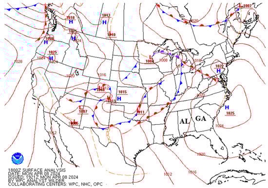
Figure 1.
Weather Prediction Center surface analysis for 1800 Universal Time Coordinate (UTC) 8 April 2024. The states of Alabama (AL) and Georgia (GA) are labeled. Red contours are isobars in hPa. Blue H’s indicate high pressure centers and red L’s mark low pressure centers. Warm fronts are marked in red, cold fronts in blue, occluded fonts in purple, and stationary fronts by alternating red and blue.
While observing the 8 April 2024 eclipse on the Columbus State University main campus, the first author noted a smoky haze against a backdrop of blue sky, interrupted by sparse cirriform clouds. Southerly winds at this time suggest that the likely source of the smoke was a prescribed fire originating from Fort Benning, which is located due south of Columbus. Prescribed fires are conducted in one-to-three-year cycles in forested environments on Fort Benning to reduce fuels for natural wildfires, control understory growth, and maintain ecosystem health (J. Parker, personal communication, April 2025) [17].
This study reports the results of a unique “natural experiment” that occurred during the 8 April 2024 eclipse. It is uncommon for nature to provide scenarios that create simultaneous control and experimental settings under equal forcing, allowing for independent evaluation of atmospheric responses. In this scenario, a narrow smoke plume passed directly over Columbus, Georgia during the eclipse. Two small datasets are used for comparison: four Georgia Weather Network (GWN) meso-net stations surrounded by trees and situated approximately 40–110 km from Columbus; and five Automated Surface Observing Stations (ASOS) located at regional airports, at a generally greater distance from Columbus. An absence of clouds (except for stray cirrus), a lack of strong temperature or moisture gradients, and a lack of mesoscale and synoptic forcing maintained the system in a more-or-less closed state. This dataset permits the testing of eclipse response under near-equal radiative forcing in three environments: smoky (Columbus), wooded clear air (GWN), and open clear air (ASOS). The goals of this paper are to highlight key results from this natural experiment; to evaluate contributions from thermal and mechanical turbulence in smoky and clear environments based on the available surface observations; and to propose a hypothesized mechanism that may partially explain the greater thermal buffering observed in a smoky environment.
2. Materials and Methods
Surface observations in the immediate Columbus, GA area during the 8 April 2024 eclipse were limited. The Columbus ASOS station (KCSG) is located at Columbus Airport, on the north side of the city and a short distance from the main campus of Columbus State University, where the first author observed the eclipse. Columbus State University operates a weather station at Oxbow Environmental Learning Center (OELC), situated on the southern side of Columbus, just outside of the northern entrance to Fort Benning and placing it much closer to the origin of the smoke plume. Reliable data are unavailable for OELC on this date due to equipment malfunction.
One-minute and five-minute data were obtained from the Iowa Environmental Mesonet (IEM) website [18] for the closest available ASOS sites in Alabama and Georgia, which include KCSG, Albany (KABY), Macon (KMCN), and Peachtree City (KFFC) in Georgia, as well as Eufaula (KEUF) in Alabama (Figure 2). Surface observations at Montgomery, AL (KMGM) were examined but were highly influenced by larger-scale weather patterns, which made the data unsuitable for comparison with the other stations.
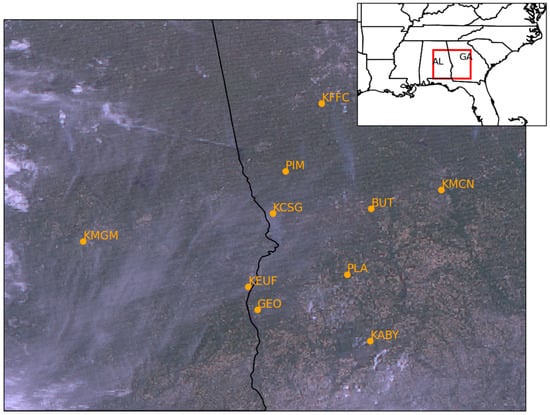
Figure 2.
True color satellite image constructed from GOES-16 channels 1, 2, and 3 at 1800 UTC 8 April 2024. The border between the states of Georgia (GA; to the east) and Alabama (AL; to the west) is shown in black. The red box in the inset map shows the domain of the satellite image. Also shown are the Automated Surface Observing Stations (ASOS) and Georgia Weather Network (GWN) stations examined in this study.
ASOS stations are sited at airports. They tend to be sited in wide-open areas with minimal tree cover. One-minute ASOS data were not available through the National Center for Environmental Information at the time of writing. The IEM one-minute temperature and dewpoint data were available at a precision of 1°F and subsequently converted to degrees Celsius. While this lack of precision limits the detection of more subtle responses, it enhances the visibility of overall trends in the data by reducing noise. Hourly ASOS data (collected from the IEM website) for several other stations in the vicinity of Columbus were examined, primarily to determine the presence of any smoke, haze, or low-level cloud cover around the time of the eclipse. The temporal resolution at these other stations was too coarse for comparison with the ASOS stations at larger airports.
The nearest surface observing stations to KCSG—Butler (BUT), Plains (PLA), Georgetown (GEO) and Pine Mountain (PIM), Georgia—are part of the Georgia Weather Network (GWN), run by the University of Georgia. The GWN stations are often situated near trees (P. Knox, personal communication, January 2025) [19]. Air temperature and dewpoint temperature are reported to the nearest hundredth of a degree Celsius, wind speed to the nearest thousandth of a meter per second, and wind direction to the nearest hundredth of a degree. The GWN stations report solar radiation but do not report cloud cover. While GWN stations offer higher precision of measurement, they report at 15-min intervals, which limits their ability to capture rapid fluctuations in eclipse-driven responses.
The 1200 Universal Time Coordinate (UTC) sounding at Peachtree City, Georgia (KFFC) on 8 April 2024 was obtained from the University of Wyoming upper air sounding archive to seek evidence of a capping inversion [20]. Geostationary Operational Environmental Satellite-16 (GOES-16) data were obtained through Amazon via the National Oceanic and Atmospheric Administration (NOAA) Weather and Climate Toolkit [21] and were used to confirm cloud cover and to seek confirmation of the smoke plume originating from the prescribed fire. ChatGPT v.4.5 facilitated the writing of Python 3 codes to display the data. All ASOS, GWN, and satellite data referenced in this publication are included in a Supplementary Materials File that accompanies this article.
3. Results
True-color satellite imagery to detect the smoke plume is unavailable during the eclipse window owing to the lack of incoming shortwave energy. In the available true- color satellite imagery from before the eclipse (Figure 2), the smoke plume is visible as an enhanced region of cloud cover immediately south of KCSG. The presence of high cloud cover makes it difficult to separate the extent of the smoke plume from the extent of the cloud cover. Per visibility observations at KCSG, the smoke dissipated at KCSG at approximately 1930 UTC.
In Columbus, the eclipse began at 1743 UTC. Solar radiation began to decrease at 1745 UTC at BUT and PIM (the nearest GWN stations to KCSG; Figure 3A). At KCSG, the maximum obscuration of 78.7% occurred at 1902 UTC. Solar radiation reached a minimum value of 186.6 W-m−2 at BUT and a minimum value of 155.3 W-m−2 at PIM, both of which occurred at 1915 UTC (Figure 3A). Solar radiation data are not available for the ASOS stations. The response in solar radiation following the eclipse indicated clear skies at all GWN stations except PIM, which is located northeast of Columbus. The cloud cover at PIM, which is located downwind of Columbus for this case, likely resulted from aerosol loading by the smoke plume. Satellite data show no evidence of either cloud cover or the smoke plume after the region emerges from the eclipse shadow. Due to the lack of observed clouds, the smoke plume is more likely to be responsible for the observed reduction in radiation at PIM beginning at 1945 UTC. More discussion of these observations is provided later in this section. The eclipse ended at 2018 UTC in Columbus. For surrounding stations, the time of maximum obscuration was within 4 min of that at KCSG, and the maximum obscuration was within 5%.
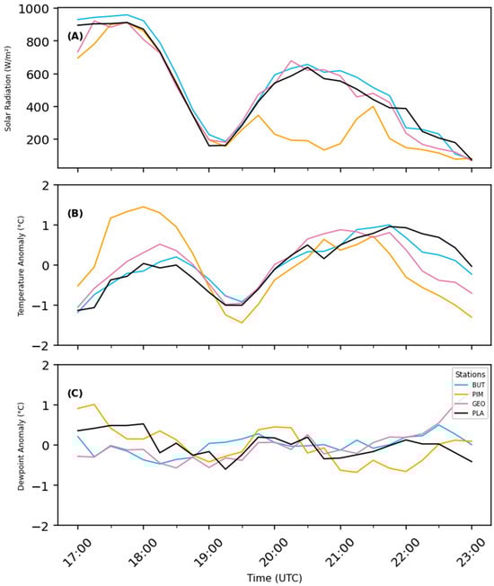
Figure 3.
Surface observations for 1700–2300 UTC 8 April 2024 at GWN stations BUT, PIM, GEO, and PLA. Panels are as follows: (A) Solar radiation (W-m−2), (B) Temperature anomaly (°C), and (C) Dewpoint temperature anomaly (°C). Anomalies are computed for each station relative to the 1700–2300 UTC mean.
The arrival of smoke at KCSG was marked by an increase in the visibility coefficient beginning at 1730 UTC, 13 min before eclipse onset (Figure 4D). Increasing visibility coefficient corresponds to a decrease in visibility. Between 1800 UTC and 1830 UTC, the visibility coefficient continued to increase at KCSG. By 1852 UTC, the KCSG temperature had reached its minimum (23.9 °C) and remained constant for the next 34 min (within the limits of precision of the temperature data; Figure 4A). This duration of constant temperature far exceeds that of surrounding ASOS stations and suggests a more rapid and stronger stabilization of the boundary layer than would be produced without a layer of smoke. The visibility coefficient began to diminish at approximately 1915 UTC (13 min after maximum obscuration), and visibility had returned to baseline by 1930 UTC, about 45–50 min before the end of the eclipse. There is no evidence that any other ASOS station was affected by smoke to the same extent as at KCSG during the eclipse.
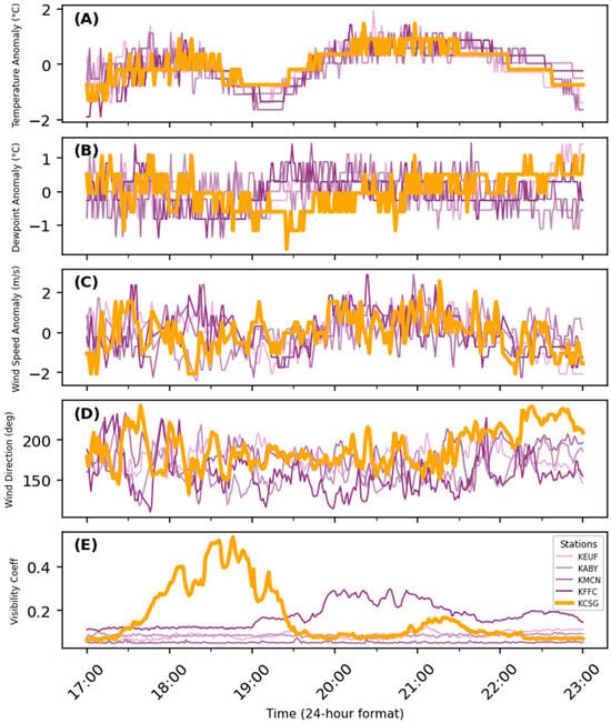
Figure 4.
Surface observations for 1700–2300 UTC 8 April 2024 at ASOS stations KCSG (bold orange-yellow line), KEUF, KABY, KMCN, and KFFC. Panels are as follows: (A) Temperature Anomaly (°C), (B) Dewpoint anomaly (°C), (C) Wind speed anomaly (m s−1), (D) Wind direction (°), (E) Visibility coefficient. Anomalies are computed for each station relative to the 1700–2300 UTC mean.
Temperature depression is defined as the difference between the maximum temperature from the two hours prior to maximum obscuration and the minimum temperature from the hour following maximum obscuration [7]. The temperature depression at KCSG was 1.7 °C. Among ASOS stations, the next closest value was 2.2 °C at KFFC and KEUF. The limited precision of ASOS temperature data may underestimate the difference in temperature depression. In comparison, the minimum temperature depression among GWN stations was 1.04 °C at PLA, and the maximum temperature depression was 2.89 °C at PIM. The wider range of temperature response at GWN stations is likely attributable, at least in part, to the variability in vegetation surrounding the stations and to the impact of the smoke plume at PIM, which was located farther downwind of the fire than KCSG. Differences in measuring equipment between ASOS and GWN stations might also contribute to the observed differences in temperature depression measurements. The temperature began to decrease at most GWN (Figure 3B) and ASOS (Figure 4A) stations between 1800 UTC and 1830 UTC and continued to fall until about 1900 UTC, at which time the temperature became constant, to the degree of precision of the one-minute ASOS data. With this lack of precision, the time from maximum obscuration to minimum temperature at KCSG cannot be determined.
Beginning at 1800 UTC, temperature and wind speed decreased at these other ASOS stations in response to reduced shortwave forcing. The other ASOS stations showed variability throughout the 34-min time period during which temperature remained constant at KCSG. The temperature began to rise at other ASOS stations around 1915 UTC and reached a relative maximum around 2030 UTC. There were no major differences in the timing of the thermal response in smoky and clear air, suggesting that changes in shortwave forcing drive temperature changes without a lagged response. All GWN stations showed similar responses in temperature, including at PIM, which experienced reduced solar radiation beginning at 1945 UTC.
The dewpoint temperature remained relatively constant at other ASOS stations (Figure 4B) before eclipse onset. In contrast, dewpoint decreased at all four GWN stations (Figure 3C) from 1800 UTC to about 1900 UTC (maximum obscuration). The dewpoint rose at most ASOS stations from 1900 to 1930 UTC and at all four GWN stations from 1930 to 2030 UTC. At KCSG, the dewpoint decreased during this window, as the visibility returned to normal. The dewpoint remained relatively lower at KCSG than at the other stations during the post-peak phase of the eclipse, until about 2010 UTC. The dewpoint decreased after 1845 UTC at all four GWN stations and remained constant at several ASOS stations (including KCSG), until about 2230 UTC, when it began to rise.
Wind data are not discussed or displayed for the GWN stations because noise and lack of temporal precision obscured any trends in the data. For the ASOS stations, wind speed (Figure 4C) responded similarly to air temperature, in that the wind speed began to trend downward beginning at 1900 UTC. The wind speed at KCSG and KABY generally increased from 1825 to 1900 UTC, while the wind speed at other ASOS stations generally decreased. At KCSG, a sudden burst of wind occurred at the time of maximum obscuration for about 15 min: the eclipse wind. The other ASOS stations showed a much weaker peak in wind speed at this time, or no peak at all. The wind speed then increased at all ASOS stations from approximately 1920 UTC to approximately 2000 UTC, likely influenced by increasing destabilization of the boundary layer as sunlight grew in intensity.
The wind direction was much less variable at KCSG following the eclipse wind until 1955 UTC. This reduction in variability of wind direction began as the smoke coverage was waning and continued after the smoke had dissipated. Veering winds occurred beginning at maximum obscuration at the ASOS stations but were more prominent beginning approximately 45 min after the end of the eclipse and continuing for about an hour. At KCSG, the wind veered from 1800 to 1930 UTC. The event concluded with nearly steady-state winds, temperature, and dewpoint.
The first author observed that a smoky haze was concentrated at the top of the boundary layer, with clear blue sky visible just above the smoke layer. This suggests that either moderate convection persisted in the boundary layer throughout the duration of the eclipse or that buoyancy was provided by the advected smoky air itself to loft the smoke to the top of the boundary layer. Alternatively, Doppler lidar observations of the boundary layer during the 21 August 2017 eclipse in Kentucky noted oscillations present throughout the boundary layer, with regular wave motions most prominent in the region of greatest static stability, which lies just below the capping inversion [5]. It is possible that these wave motions at that height, if present, might have helped to maintain peak concentration of smoke at the top of the boundary layer. The 1200 UTC KFFC sounding (Figure 5) featured a prominent capping inversion at approximately 1.2 km, which is in line with the estimated height of the smoke as viewed by the first author and with the cloud cover reports shown in Figure 6 and discussed below.
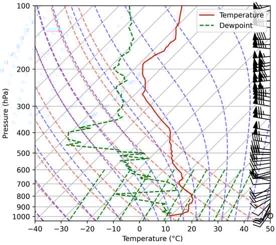
Figure 5.
The KFFC sounding for 1200 UTC 8 April 2024. The capping inversion is located at approximately 1.2 km altitude. The bold, solid red line represents air temperature and the bold, dashed green line represents dewpoint temperature. Dashed red lines, dashed green lines, and straight dashed green lines represent dry adiabats, moist adiabats, and constant mixing ratio, respectively.
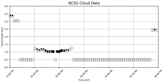
Figure 6.
Cloud cover observations at KCSG from 1700 UTC 8 April 2024 to 2300 UTC 8 April 2024. Empty circles represent clear skies. Circles with one vertical line represent few clouds (approximately 1/8 coverage). Quarter-filled symbols with a downward line represent scattered clouds (approximately 3/8 coverage). Half-filled symbols with a horizontal line represent broken clouds (approximately 5/8 coverage). Completely filled circles represent overcast skies (8/8 coverage).
In general, sky conditions across western Georgia and eastern Alabama were mostly reported as clear throughout the duration of the 8 April 2024 eclipse. At KCSG, clouds were reported at approximately 3-km elevation around 1700 UTC and later in the day between 2100 and 2200 UTC, as is shown in Figure 6. These reports did not include the cirriform clouds visible in satellite data approaching from the west, as they likely exceeded the vertical range of the ceilometer. KCSG reported a growing blanket of clouds (Figure 6) at the approximate height of the capping inversion from 1800 to 1930 UTC, in agreement with the reported changes in visibility during this time. No clouds at such a height were visible to the first author at this time, suggesting that the ceilometer was likely detecting an elevated layer of haze rather than true cloud. Roughly coincident with the cloud reports, haze at the surface was reported at KCSG from 1805 to 1920 UTC. Haze is reported when the ASOS visibility sensor detects a reduction in light scattering by particles too small to be detected by the present weather sensor [22]. Furthermore, a haze report must occur in a relatively dry environment.
As shown by the reports in Figure 6, this blanket of haze grew in coverage and lowered in height until 1845 UTC and then receded in coverage while rising in height from 1855 to 1930 UTC. Mixing layer depth and cloud base height have been commonly shown to follow this pattern during eclipses [10,23]. The cloud growth process was interrupted by a (likely spurious) report of clear skies at 1850 UTC. The reported cloud heights suggest a maximum smoke plume rise of 1.3 km, as indicated by the KCSG cloud reports, which aligns with the typical value for prescribed burns of approximately 1 km [24]. Although Pasken et al. [16] noted a much more rapid decrease in boundary layer height, the timing of the KCSG cloud cover reports aligns with the timing of surface reports of haze but not with the timing of the eclipse maximum, supporting the interpretation of a smoke plume advecting over the area. In a similar instance of a spurious cloud report, Evan et al. [25] noted the misidentification of a dust cloud as a cloud by an Aerosol Robotic Network (AERONET) station in southeastern California.
4. Discussion
4.1. Turbulent Processes
The key to understanding how weather parameters respond differently in smoky and clear environments lies in Segal et al.’s [26] assertion that more thermal energy is required to dissipate a morning surface inversion in a smoky environment than a clear one. Observations of reduced thermal turbulence [10] and a stabilizing boundary layer [15] during eclipses suggest that the dissipation of thermal and mechanical turbulence lowers the ratio of active to stored energy, as much of the dissipated energy must remain in the system. During the 21 August 2017 solar eclipse, the greatest decay in TKE was found to occur near and just after totality [14]. Turbulent mixing in the boundary layer has been found to lag behind responses in surface fluxes after an eclipse [15]. The eclipse-altered energy budget in a smoky environment likely influences not only surface fluxes but also the vertical distribution of stability and boundary layer height, altering the post-eclipse increase in mixing as convection resumes [5]. In addition, incoming shortwave energy is more likely to be stored above the surface via shortwave absorption by aerosols higher in the boundary layer [27]. This storage of energy aloft may affect boundary layer lapse rates, suppressing the post-eclipse convective response to a greater extent in a smoky environment.
4.1.1. Thermal Turbulence
The contemporaneous changes across several variables at multiple times in response to changing shortwave forcing (Section 4.2) points to likely changes in the turbulence regimes. Previous work has shown that turbulence goes through several stages of suppression and recovery during and after an eclipse [14]. That these changes were simultaneous between smoky and clear environments suggests that these turbulent transitions are solely dependent on timing of the shortwave forcing, with no lagged effects imposed by differences in the thermodynamic environment. It has been shown by measurements of turbulent fluxes and momentum that turbulent transitions during an eclipse are driven primarily by radiative forcing rather than by local environmental factors [14].
Figure 7 displays a qualitative timeline of the 8 April 2024 event from 1700 to 2100 UTC. The shortwave radiation forcing is indicated from the beginning of the eclipse (first contact) to the end of the eclipse (last contact). The smoke forcing is shown in red for the time during which the visibility coefficient at KSCG was above the baseline, as indicated in Figure 4E. GWN stations are excluded from the analysis because the 15-min reporting interval is too broad to determine variability.
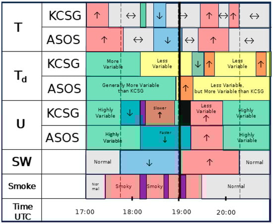
Figure 7.
Timeline from 1700 UTC to 2100 UTC 8 April 2024 showing key changes in air temperature (T), dewpoint temperature (Td), and wind speed (U) observations at KCSG and other ASOS stations, along with three forcings: shortwave radiation (SW), smoke (at KCSG only), and urban heat island effect (UHI). Tick marks are provided at each hour. Dashed lines represent the duration of the eclipse. The bold line at 1902 UTC indicates the time of maximum obscuration. Up arrows (red) represent an increase in the variable’s magnitude, down arrows (blue) represent a decrease in the variable’s magnitude, and sideways arrows (pink) represent little to no overall change. Normal shortwave and visibility conditions (smoke) are also denoted by pink boxes. The black box at 1902 UTC indicates the eclipse wind at KCSG. The dark purple boxes represent a brief “dip” in a parameter. The green box at 1800 UTC in the KCSG temperature indicates a brief increase in temperature variability. The tone of red and blue boxes may be slightly altered if they are overlaid on yellow or green boxes.
Before eclipse onset, normal temperature behavior—diurnal warming—occurred. This warming process suggests a build-up of thermal turbulence and a convectively active boundary layer [10]. The increase in temperature variability indicated by the green box in temperature at around 1810 UTC (Figure 7) suggests a brief interval of enhanced thermal turbulence, potentially due to uneven surface heating and influenced by the smoky environment. It is also possible that an aerosol-moisture feedback (described in Section 4.3) also plays a role, as the visibility coefficient oscillated at this time. Mahmood et al. [5] found localized variability in near-surface temperature and turbulence, attributed to inhomogeneous land-surface conditions [5].
As the eclipse peak approached, a threshold in boundary layer stability may have been reached, leading to decreasing temperature after this time. Observations from the 15 January 2010 annular solar eclipse over India note a change in the boundary layer lapse rate from unstable to neutral and a substantial drop in both the skin temperature and the 1-m air temperature at this stage of the eclipse [9]. At KCSG, reduced shortwave forcing at this time likely contributed to the sustained reduction of thermal turbulence and the suppression of boundary layer mixing, as has been observed by Turner et al. [15]. The post-eclipse increase in thermal turbulence appears to require multiple periods of adjustment at KCSG, as indicated by the intervals of near-constant temperature that interrupt its gradual rise. A gradual post-peak temperature recovery was also shown for the 21 August 2017 eclipse [14]. At KCSG, these additional periods of adjustment may be associated with a multi-stage breakdown of layers of stability, which were likely stronger in the smoky environment of KCSG than in the clear environment of the other ASOS stations. Previous work has shown that a surface layer and a residual layer separated by either an inversion or a shear layer may form during an eclipse, leading to decoupled flow [10,14]. Recent UAV observations confirm that distinct responses occur as a function of height in the boundary layer, with rapid changes in the surface layer and a slower response at upper levels [16]. A staggered breakdown of inversions in the surface and residual layers may have contributed to the post-peak temperature adjustments observed at KCSG.
4.1.2. Mechanical Turbulence
Changes in mechanical turbulence may also be inferred from the behavior of surface parameters before, during, and after an eclipse. For example, the transition from a convective to a stable regime has been shown to suppress both buoyant and mechanical turbulence near the surface [14]. Variability in wind speed was high before 1800 UTC, suggesting strong mechanical mixing pre-eclipse. This mixing may be generated by building diurnal convective activity and thermal turbulence, and also by mechanical shear-generated turbulence [14]. Pre-eclipse conditions have been shown to be dominated by convective turbulence, with high TKE and turbulent mixing [14]. At KCSG, the onset of smoke and the beginning of the eclipse appear to dampen this mechanical turbulence, as the wind speed decreases in response to decreased shortwave forcing [9].
A sudden peak in wind speed at 1810 UTC might be attributed to downward mixing of momentum, as momentum from a faster-moving layer aloft is brought to the surface. The wind speed variability suddenly decreases after 1810 UTC, then begins a gradual upward trend. This appears to mark a shift to a mechanically-dominated turbulence regime, in which cooling likely begins to suppress convection and buoyant turbulence. Reduced convective activity in a cooling environment would indicate a transition to a more stable boundary layer [14]. The reduced variability in wind speed indicates that the flow likely becomes more laminar, with fewer intrusions of turbulent eddies. Thus, the wind speed would gradually accelerate in an increasingly stratified environment. This would produce a decoupled flow pattern (as described at the end of Section 4.1.1) dominated by mechanical turbulence [14]. Increased wind speed was observed at KCSG immediately after the peak in wind speed at 1810 UTC.
From eclipse peak at 1902 UTC until about 1930 UTC, wind speed continues to increase. Due to increasing shortwave forcing, surface warming resumes, mixing layers re-establish, and convective turbulence grows, producing a gradual increase in mechanical turbulence [14]. By 2000 UTC, increased variability in wind speed at KCSG suggests the establishment of a new turbulent regime [15]. Overall, lagged temperature recovery in the smoky environment at KCSG suggests a longer period of mechanical turbulence suppression and recovery, likely driven by increased atmospheric stability. In a clear eclipse environment, clouds and high surface moisture can enhance cooling and suppress turbulence, particularly over vegetated surfaces [8]. At KCSG, smoke performs a similar role.
4.2. Aerosol Influences on Thermal Response
Ultimately, the differences between the conditions at KCSG and those at other ASOS stations result from the incursion of smoke aerosols at KCSG. In general, aerosols are measured with respect to two threshold diameters: particles ≤10 µm (PM10) and those ≤2.5 µm (PM2.5). Smoke particles fall into the PM2.5 category, with a median diameter between 50 and 200 nm [28,29]. In this section, we review the literature to explore the expected thermal response to smoke aerosols at KCSG and to determine whether this predicted response supports the observations of a warmer temperature depression and an extended steady-state temperature condition.
Studies of aerosol contributions to urban heat islands offer insights into the influence of particle size on boundary layer thermal response under changing radiative forcing. Measurements of the urban heat island in a semi-arid environment, where dust particles (PM10) dominate, and in a polluted urban environment, where smaller particles (PM2.5) dominate, can show the contribution of aerosols to urban heat island intensity (UHII) as a function of aerosol size. UHII represents the difference in temperature between an urban environment and the surrounding rural environment. Previous work has found that smaller particles are associated with a lower UHII [30]. This suggests little difference in temperature depression between the smoky environment at KCSG and the clear environment at the other ASOS stations owing to the small diameter of smoke particulates. In general, UHII tends to be greater during nighttime [31,32], due to increased retention of heat within the air in urban environments in the absence of sunlight. Therefore, the influence of smoke aerosols during an eclipse may increase as the shortwave forcing decreases.
The earliest studies of smoke’s influence on temperature examined the effects of large forest fires, with the aim of understanding the possible consequences of a “nuclear winter” in the event of a nuclear war [33,34]. During a wildfire, the primary effect of a thick daytime smoke layer on shortwave radiation is to increase the albedo relative to that of the forest and, in turn, to produce cooling [34]. It has been known for some time that the reduction in insolation provided by wildfire smoke is capable of extending the lifetime of inversions in the boundary layer in a process known as smoke shading [27,34,35]. In the case of an eclipse in a smoky environment, one would expect that the cooling effect of enhanced albedo would amplify cooling at smoky stations relative to clear stations. The warming observed at KCSG suggests that the albedo is weaker in the thinner, hazy environment during the eclipse than what is typical of dense wildfire smoke. Any albedo-induced cooling at KCSG must have been overridden by other processes created by the changing shortwave forcing during the eclipse.
Few studies explore the direct relationship between infrared radiation and smoke, and those that exist study daytime conditions or utilize a controlled setting. Observing the passage of a dense smoke layer on an otherwise clear morning, Hand [36] found that smoke particles have little to no measurable effect on infrared radiation, concluding that smoke does not significantly absorb longwave energy. In laboratory thermal imaging experiments, Li et al. [37] showed that absorption by smoke is negligible at thermal infrared wavelength; their measurements found that the attenuation due to absorption obeys Beer’s Law. Their study was unrepresentative of natural conditions in that it investigated only one smoke concentration, and the chemical composition of the smoke may not reflect smoke from wildfires or prescribed fires. While limited, these studies do not support a measurable “insulating effect” by infrared radiation as the cause of the relatively mild eclipse response at KCSG. Taken a step further, these results suggest that vertical variations in the absorption of infrared radiation may not substantially contribute to increased stability in a smoky eclipse environment. Consequently, there is a need to examine alternative mechanisms that might help to explain the thermal buffering observed at KCSG.
Shortwave absorption by black carbon may play a role in increasing temperature in a smoky boundary layer. However, Bernhard and Petkov [38] observed increased diffuse irradiance under high aerosol concentrations during the 21 August 2017 eclipse. This suggests that the smoky environment at KCSG may produce increased scattering and reduced absorption at infrared wavelengths. Other processes, such as surface heterogeneity [9], enhanced decoupling of the boundary layer [35], or delayed breakup of the inversion layer [26], may also contribute to the mild thermal response at KCSG. Section 4.3 proposes an alternative mechanism (the Subcritical Aerosol-Moisture Feedback; SAMF) that may contribute to the observations of steady-state thermodynamic conditions during the time of peak eclipse. Latent heat release via hygroscopic aerosol growth may further play a role in this newly proposed mechanism.
4.3. The Subcritical Aerosol-Moisture Feedback
Key transitions in the response of surface parameters occurred simultaneously in smoky and clear environments, marking different stages of the 8 April 2024 eclipse (Figure 7). For both environments, the temperature responded by leveling off within minutes of the reduction in forcing. This occurred earlier at KCSG due to the arrival of smoke. The first transition after the initial temperature response occurred at approximately 1810 UTC at all ASOS stations, including KCSG. The visibility coefficient at KCSG displayed a sharp departure from its rising trend, with the coefficient briefly reduced and visibility temporarily increased. Corresponding with this short-lived increase in visibility, a brief dip occurred in the wind speed at KCSG, marking a change from decreasing to increasing wind speed. This increase in wind speed was also noted for the 2017 Great American eclipse in Oklahoma [15]. Also at 1810 UTC, the temperature variability peaked briefly, and the dewpoint became less variable. At the other ASOS stations, wind speeds began to decelerate until after eclipse maximum, as Gray and Harrison [12] found for the 20 March 2015 eclipse over the British Isles.
At eclipse maximum, a second transition occurred. The eclipse wind was evident at KCSG, even though the surface temperature and dewpoint remained nearly constant. This steady-state condition around the time of peak eclipse suggests that a thermodynamic buffering mechanism was active. Visibility fluctuations during this time of near-constant moisture hint at rapid changes in aerosol scattering properties. In general, aerosol particles scatter much more light than they absorb, and the amount of scattering is highly sensitive to relative humidity [39]. We propose that this steady-state condition may be produced by a possible aerosol-moisture feedback—the SAMF—among aerosols of different size or composition. The SAMF involves responses between aerosol size, relative humidity, and the scattering of radiation that regulate temperature and humidity, especially in subsaturated, aerosol-laden environments. Such a population-wide evolution in aerosol size distribution might provide a thermodynamically stabilizing mechanism, wherein the changing spatial distribution of latent heating regulates relative humidity, while simultaneously influencing visibility by altering radiative scattering and absorption.
In the smoky environment at KCSG, such an effect would be amplified by a high aerosol count and a broader aerosol size distribution, which could further buffer the thermodynamic environment against change. Aerosols modulate the surface radiation budget, and they can alter the vertical thermodynamic structure of the boundary layer [40]. In the traditional model of aerosol growth, relative humidity is directly related to aerosol size and aerosol scattering [41]. However, aerosol optical properties are highly sensitive to small changes in relative humidity, which suggests a potential for nonlinear effects due to moisture perturbations [39]. Aerosol particles can retain liquid water features down to 33% relative humidity and can demonstrate rapid moisture exchange between particles [42]. Organic acids, in particular, play a role in hygroscopic aerosol growth in three ways: (1) they help to determine an aerosol’s uptake of water, particularly at lower humidity; (2) their interactions with inorganic salts influence hygroscopic particle growth; and (3) chemical reactions within smoke aerosols can alter their composition and moisture exchange with the environment [43]. As aerosols grow, they are subject to competing processes: augmentation of an aerosol’s coating, which amplifies absorption, and assimilation of refractive index, which decreases absorption. These competing effects may provide a mechanism by which aerosol growth actively moderates atmospheric moisture and latent heat production, particularly in transient environments with higher aerosol concentrations [39]. In short, dynamic exchanges between aerosols and relative humidity may help to dampen changes in the thermodynamic environment during transient events such as an eclipse.
The proposed mechanism of the SAMF operates as follows during the 8 April 2024 eclipse. As temperature decreases during the pre-peak phase of the eclipse, relative humidity rises, producing growth of aerosol particle size, especially in a smoky environment. The increased water content of the aerosols alters their growth dynamics and their scattering properties, producing fluctuations in visibility. The associated release of latent heat subtly modifies the thermodynamic structure of the boundary layer. These changes to the environment alter the relative humidity, modifying conditions that produce additional growth or shrinkage. These changes complement each other to maintain the surface temperature and moisture at a steady-state condition.
5. Conclusions
This paper examines surface observations during the solar eclipse on 8 April 2024 in Columbus, Georgia, where smoke from a nearby prescribed fire influenced the boundary layer response to rapid shortwave radiation loss. Ideal weather conditions and a near-Gaussian smoke incursion make this case a highly idealized natural experiment through which to explore the influence of smoke during a rapid, transient change in shortwave radiation relative to clear conditions. The effect of the smoke at KCSG was to produce a temperature depression that was approximately 0.5 °C warmer than at surrounding ASOS stations. At GWN meso-net stations, where vegetation was more extensive, the temperature depression also tended to be reduced, illustrating that the surface layer response is highly sensitive to the local environment under rapid shortwave forcing. In the smoky environment at KCSG, surface responses were more complex than at other ASOS stations: the eclipse wind was more pronounced, and the post-eclipse warming was notably delayed. Despite the additional complexity of the response in the smoky environment, the timing of transitions between turbulence regimes was unaffected by smoke.
We have proposed that population dynamics of aerosol growth and their influence on moisture in the environment may help to reinforce steady-state conditions in temperature and dewpoint at the surface during the peak phase of the eclipse. Future work could test this hypothesis by analyzing high-resolution visibility and aerosol data throughout eclipse periods under both clear and smoky conditions. Evidence for this phenomenon could be obtained by instruments such as aerosol counters and particle sizers, which could measure changes in aerosol size distributions. Flux tower measurements of latent heat in the boundary layer under smoky conditions could provide evidence for the role of subtle fluctuations in latent heating. Similarly, the use of hygrometers on unmanned aerial vehicle (UAV) flights could determine whether a subtle vertical redistribution of moisture or latent heat occurs, particularly near eclipse maximum. Integrating such findings into numerical simulations that account for changes in aerosol size may offer a theoretical means to test the plausibility of the proposed Subcritical Aerosol-Moisture Feedback (SAMF) response between aerosol growth and relative humidity. By considering boundary layer processes, aerosols, and eclipse-induced radiative fluxes in smoky and clear environments, this study offers a novel framework for future research. We hope that our approach leads to new insights into how the interactions between aerosols, moisture, and radiation shape boundary layer conditions, particularly during eclipses.
Supplementary Materials
The following supporting information can be downloaded at: https://www.mdpi.com/article/10.3390/atmos16050578/s1. Supplementary Materials File.
Author Contributions
Conceptualization, S.M.J.; Data curation, B.B.E.; Methodology, S.M.J.; Project administration, S.M.J.; Supervision, S.M.J.; Visualization, S.M.J.; Writing—original draft, S.M.J.; Writing—review and editing, S.M.J. All authors have read and agreed to the published version of the manuscript.
Funding
This project received no external funding.
Institutional Review Board Statement
Not applicable.
Informed Consent Statement
Not applicable.
Data Availability Statement
The original contributions presented in this study are included in the Supplementary Materials. Further inquiries can be directed to the corresponding author.
Acknowledgments
The authors thank James Parker, Pamela Knox, and Shawn Milrad for conversations and feedback that enhanced the manuscript. ChatGPT v4.5 provided assistance in generating Figure 2, Figure 3, Figure 4, Figure 5 and Figure 6. Microsoft Powerpoint was used to generate Figure 7. ChatGPT v4.5 was also used to search the literature [Section 4.1 and articles [39,40,41,42,43] and to facilitate wordsmithing [Section 3, Section 4 and Section 5]]. This research is supported by the Columbus State University Earth and Space Sciences (ESS) Foundation.
Conflicts of Interest
The authors declare no conflicts of interest.
Correction Statement
This article has been republished with a minor correction in the Abstract. This change does not affect the scientific content of the article.
References
- Anderson, J. Meteorological changes during a solar eclipse. Weather 1999, 54, 207–215. [Google Scholar] [CrossRef]
- Aplin, K.L.; Scott, C.J.; Gray, S.L. Atmospheric changes from solar eclipses. Philos. Trans. R. Soc. A 2018, 374, 20150217. [Google Scholar] [CrossRef] [PubMed]
- Hanna, E.; Penman, J.; Jónsson, T.; Bigg, G.R.; Björnsson, H.; Sjúrðarson, S.; Hansen, M.A.; Cappelen, J.; Bryant, R.G. Meteorological effects of the solar eclipse of 20 March 2015: Analysis of UK Met Office automatic weather station data and comparison with automatic weather station data from the Faroes and Iceland. Philos. Trans. R. Soc. 2016, 374A, 20150212. [Google Scholar] [CrossRef]
- Fowler, J.; Wang, J.; Ross, D.; Colligan, T.; Godfrey, J. Measuring ARTSE2017 Results from Wyoming and New York. Bull. Am. Meteorol. Soc. 2019, 100, 1049–1060. [Google Scholar] [CrossRef]
- Mahmood, R.; Schargorodski, M.; Rappin, E.; Griffin, M.; Collins, P.; Knupp, K.; Quilligan, A.; Wade, R.; Cary, K. The Total Solar Eclipse of 2017 Meteorological Observations from a Statewide Mesonet and Atmospheric Profiling Systems. Bull. Am. Meteorol. Soc. 2020, 101, E720–E737. [Google Scholar] [CrossRef]
- Gross, P.; Hense, A. Effects of a total solar eclipse on the mesoscale atmospheric circulation over Europe—A model experiment. Meteorol. Atmos. Phys. 1999, 71, 229–242. [Google Scholar] [CrossRef]
- Dodson, J.B.; Robles, M.C.; Taylor, J.E.; DeFontes, C.C.; Weaver, K.L. Eclipse across America: Citizen Science Observations of the 21 August 2017 Total Solar Eclipse. J. Appl. Meteorol. Climatol. 2019, 58, 2363–2385. [Google Scholar] [CrossRef]
- Ahrens, D.; Iziomon, M.G.; Jaegar, L.; Matzarakis, A.; Mayer, H. Impacts of the solar eclipse of 11 August 1999 on routinely recorded meteorological and air quality data in south-west Germany. Meteorol. Z. 2001, 10, 215–223. [Google Scholar] [CrossRef]
- Bhat, G.S.; Jagannathan, R. Moisture depletion in the surface layer in response to an annular eclipse. J. Atmos. Sol. Terr. Phys. 2017, 80, 60–67. [Google Scholar] [CrossRef]
- Burt, S. Meteorological responses in the atmospheric boundary layer over southern England to the deep partial eclipse of 20 March 2015. Philos. Trans. R. Soc. A 2016, 374, 20150214. [Google Scholar] [CrossRef]
- Eaton, F.D.; Hines, J.R.; Hatch, W.H.; Cionco, R.M.; Byers, J.; Garvey, D. Solar eclipse effects observed in the planetary boundary layer over a desert. Bound. Layer Meteorol. 1996, 83, 331–346. [Google Scholar] [CrossRef]
- Gray, S.L.; Harrison, R.G. Eclipse-induced wind changes over the British Isles on the 20 March 2015. Philos. Trans. R. Soc. A 2016, 374, 20150224. [Google Scholar] [CrossRef] [PubMed]
- Winkler, P.; Kaminski, U.; Köhler, U.; Riedl, J.; Schroers, H.; Anwender, D. Development of meteorological parameters and total ozone during the total solar eclipse of August 11, 1999. Meteorol. Z. 2001, 10, 193–199. [Google Scholar] [CrossRef]
- Bailey, S.C.; Canter, C.A.; Sama, M.P.; Houston, A.L.; Smith, S.W. Unmanned aerial vehicles reveal the impact of a total solar eclipse on the atmospheric surface layer. Proc. R. Soc. A 2019, 475, 20190212. [Google Scholar] [CrossRef]
- Turner, D.D.; Wulfmeyer, V.; Behrendt, A.; Bonin, T.A.; Choukulkar, A.; Newsom, R.K.; Brewer, W.A.; Cook, D.R. Response of the land-atmosphere system over north-central Oklahoma during the 2017 eclipse. Geophys. Res. Lett. 2018, 45, 1668–1675. [Google Scholar] [CrossRef]
- Pasken, R.; Woodford, R.; Bergmann, J.; Hickel, C.; Ideker, M.; Jackson, R.; Rotter, J.; Schaefer, B. Effects of the 2024 Total Solar Eclipse on the Structure of the Planetary Boundary Layer: A Preliminary Analysis. Atmosphere 2024, 15, 1008. [Google Scholar] [CrossRef]
- Parker, J.M. (Directorate of Public Works, Fort Benning, GA, USA). Personal communication, 2025.
- Iowa Environmental Mesonet. Available online: https://mesonet.agron.iastate.edu/ASOS (accessed on 28 March 2025).
- Knox, P.N. (University of Georgia, Athens, GA, USA). Personal communication, 2025.
- University of Wyoming Atmospheric Science Radiosonde Archive. Available online: https://weather.uwyo.edu/upperair/sounding.shtml (accessed on 28 March 2025).
- Ansari, S.; Del Greco, S.; Kearns, E.; Brown, O.; Wilkins, S.; Ramamurthy, M.; Weber, J.; May, R.; Sundwall, J.; Layton, J.; et al. Unlocking the Potential of NEXRAD Data through NOAA’s Big Data Partnership. Bull. Am. Meteorol. Soc. 2018, 99, 189–204. [Google Scholar] [CrossRef]
- National Weather Service. ASOS (Automated Surface Observing System) User’s Guide; NOAA, U.S. Department of Commerce: Washington, DC, USA, 1998; p. 38. [Google Scholar]
- Mishra, M.K.; Rajeev, K.; Nair, A.K.M.; Moorthy, K.K.; Parameswaran, K. Impact of a noon-time annular solar eclipse on the mixing layer height and vertical distribution of aerosols in the atmospheric boundary layer. J. Atmos. Sol. Terr. Phys. 2017, 74, 232–237. [Google Scholar] [CrossRef]
- Liu, Y. A Regression Model for Smoke Plume Rise of Prescribed Fires Using Meteorological Conditions. J. Appl. Meteorol. Climatol. 2019, 53, 1961–1975. [Google Scholar] [CrossRef]
- Evan, A.; Walkowiak, B.; Frouin, R. On the Misclassification of Dust as Cloud at an AERONET Site in the Sonoran Desert. J. Atmos. Ocean. Technol. 2022, 39, 181–191. [Google Scholar] [CrossRef]
- Segal, M.; Weaver, J.; Purdom, J.F.W. Some Effects of the Yellowstone Fire Smoke Plume on Northeast Colorado at the End of Summer 1988. Mon. Weather Rev. 1989, 117, 2278–2284. [Google Scholar] [CrossRef]
- Robock, A. Surface cooling due to forest fire smoke. J. Geophys. Res. 1991, 96, 20869–20878. [Google Scholar] [CrossRef]
- Carrico, C.M.; Prenni, A.J.; Kreidenweis, S.M.; Levin, E.J.T.; McCluskey, C.S.; DeMott, P.J.; McMeeking, G.R.; Nakao, S.; Stockwell, C.; Yokelson, R.J. Rapidly evolving ultrafine and fine mode biomass smoke physical properties: Comparing laboratory and field results. J. Geophys. Res. Atmos. 2018, 121, 5750–5768. [Google Scholar] [CrossRef]
- Laing, J.R.; Jaffe, D.A.; Hee, J.R. Physical and optical properties of aged biomass burning aerosol from wildfires in Siberia and the Western USA at the Mt. Bachelor Observatory. Atmos. Chem. Phys. 2018, 16, 15185–15197. [Google Scholar] [CrossRef]
- Cao, C.; Lee, X.; Liu, S.; Schultz, N.; Xiao, W.; Zhang, M.; Zhao, L. Urban heat islands in China enhanced by haze pollution. Nat. Commun. 2016, 7, 12509. [Google Scholar] [CrossRef]
- Nguyen, L.H.; Henebry, G.M. Urban Heat Islands as Viewed by Microwave Radiometers and Thermal Time Indices. Remote Sens. 2018, 8, 831. [Google Scholar] [CrossRef]
- Han, W.; Li, Z.; Wu, F.; Zhang, Y.; Guo, J.; Su, T.; Cribb, M.; Fan, J.; Chen, T.; Wei, J.; et al. The mechanisms and seasonal differences of the impact of aerosols on daytime surface urban heat island effect. Atmos. Chem. Phys. 2020, 20, 6479–6493. [Google Scholar] [CrossRef]
- Penner, J.E.; Haselman, L.C.; Edwards, L.L. Smoke-Plume Distributions above Large-Scale Fires: Implications for Simulations of “Nuclear Winter”. J. Appl. Meteorol. Climatol. 1986, 25, 1434–1444. [Google Scholar] [CrossRef]
- Robock, A. Enhancement of surface cooling due to forest fire smoke. Science 1988, 242, 911–913. [Google Scholar] [CrossRef]
- Pahlow, M.; Kleissl, J.; Parlange, M.B.; Ondov, J.M.; Harrison, D. Atmospheric boundary-layer structure observed during a haze event due to forest-fire smoke. Bound. Layer Meteorol. 2005, 114, 53–70. [Google Scholar] [CrossRef]
- Hand, I.F. Transmission of the Total and the Infrared Component of Solar Radiation Through a Smoky Atmosphere. Bull. Am. Meteorol. Soc. 1943, 24, 201–204. [Google Scholar] [CrossRef]
- Li, H.; Wen, S.; Li, S.; Wang, H.; Geng, X.; Wang, S.; Zhai, J.; Zhang, W. The research on infrared radiation affected by smoke or fog in different environmental temperatures. Nat. Sci. Rep. 2024, 14, 14410. [Google Scholar] [CrossRef] [PubMed]
- Bernhard, G.; Petkov, B. Measurements of spectral irradiance during the solar eclipse of 21 August 2017: Reassessment of the effect of solar limb darkening and of changes in ozone. Atmos. Chem. Phys. 2019, 19, 4703–4719. [Google Scholar] [CrossRef]
- Nessler, R.; Weingartner, E.; Baltensperger, U. Effect of humidity on aerosol light absorption and its implications for extinction and the single scattering albedo illustrated for a site in the lower free troposphere. J. Aerosol Sci. 2005, 36, 958–972. [Google Scholar] [CrossRef]
- Yang, Y.; Ni, C.; Jiang, M.; Chen, Q. Effects of aerosols on the atmospheric boundary layer temperature inversion over the Sichuan Basin, China. Atmos. Environ. 2021, 262, 118647. [Google Scholar] [CrossRef]
- Jung, C.H.; Yoon, Y.J.; Um, J.; Lee, S.S.; Han, K.M.; Shin, H.J.; Lee, J.Y.; Kim, Y.P. Approximated expression of the hygroscopic growth factor for polydispersed aerosols. J. Aerosol Sci. 2021, 151, 105670. [Google Scholar] [CrossRef]
- Cziczo, D.J.; Nowak, J.B.; Hu, J.H.; Abbatt, J.P.D. Infrared spectroscopy of model tropospheric aerosols as a function of relative humidity: Observation of deliquescence and crystallization. J. Geophys. Res. Atmos. 1997, 102, 18843–18850. [Google Scholar] [CrossRef]
- Tan, F.; Zhang, H.; Xia, K.; Jing, B.; Li, X.; Tong, S.; Ge, M. Hygroscopic behavior and aerosol chemistry of atmospheric particles containing organic acids and inorganic salts. NPJ Clim. Atmos. Sci. 2004, 7, 203. [Google Scholar] [CrossRef]
Disclaimer/Publisher’s Note: The statements, opinions and data contained in all publications are solely those of the individual author(s) and contributor(s) and not of MDPI and/or the editor(s). MDPI and/or the editor(s) disclaim responsibility for any injury to people or property resulting from any ideas, methods, instructions or products referred to in the content. |
© 2025 by the authors. Licensee MDPI, Basel, Switzerland. This article is an open access article distributed under the terms and conditions of the Creative Commons Attribution (CC BY) license (https://creativecommons.org/licenses/by/4.0/).