Article

Dispersion Modeling of Odor Emissions from Area Sources in a Municipal Wastewater Treatment Plant

by
Cristian Constantin
1,2,
Cristina Modrogan
2,
Annette Madelene Dancila
2,*,
Georgeta Olguta Gavrila
1,2,
Simona Mariana Calinescu
1,2,
Alexandru Cirstea
1,
Valeriu Danciulescu
1,
Gheorghita Tanase
1 and
Gabriela Geanina Vasile
1,*
1
National Research and Development Institute for Industrial Ecology-ECOIND, 57-73, Drumul Podu Dâmboviței Street, Sector 6, 060652 Bucharest, Romania
2
Faculty of Chemical Engineering and Biotechnologies, National University of Science and Technology Politehnica Bucharest, Gheorghe Polizu Street, No. 1-7, 011061 Bucharest, Romania
*
Authors to whom correspondence should be addressed.
Atmosphere 2025, 16(5), 577; https://doi.org/10.3390/atmos16050577
Submission received: 1 April 2025 / Revised: 25 April 2025 / Accepted: 6 May 2025 / Published: 12 May 2025
(This article belongs to the Special Issue Environmental Odour (2nd Edition))

Abstract

:
Wastewater treatment plants (WWTPs) generate significant emissions of gaseous substances, such as H2S, NH3, and VOCs, which cause discomfort and pose health risks to residents in surrounding areas. The objective of this study was to estimate pollutant concentrations under various scenarios through a mathematical modeling of the pollutant dispersion in the surrounding air using the AERMOD View software platform, version 11.2.0. In this study, four mathematical models with two different scenarios were conducted to illustrate the odor concentrations both on site and in nearby areas under the most unfavorable weather conditions. The “1st Highest Values” and “98th Percentile” metrics were used to represent the peak concentrations and to exclude the 2% of conditions with the worst-case dispersion, respectively. In the first scenario, under normal operating conditions with all treatment equipment functioning, the maximum on-site odor concentration was estimated at 36.8 ouE/m3 using the 1st highest value function, and it was 20.4 ouE/m3 using the 98th percentile function. The second scenario considered all emission sources, with the grease collection system of the de-sanding/grease separation Unit Line 1 and the sludge collection system of the primary settling decanter (Unit 4) out of service. In this case, the maximum on-site odor concentration reached 749 ouE/m3 over 98% of a one-year period and 956.5 ouE/m3 using the 1st highest value function. These findings underscore the necessity for ongoing monitoring, strict adherence to environmental regulations, and stakeholder engagement to improve mitigation techniques and foster community trust in environmental management. Regular inspections are essential to ensure that all equipment operates within normal parameters, supporting both regulatory compliance and improved operational efficiency, including the control of odor emissions.

1. Introduction

Air pollution from industrial sources is one of the most pressing environmental issues in many countries [1]. Air quality and pollution levels (physical, chemical, and biological) have a significant impact on the health and survival of humans, animals, and the plants exposed to them [2].
A variety of atmospheric parameters, including temperature, wind speed, wind direction, precipitation, and relative humidity, influence aerosol dispersal and microbe survival [3]. Odorous gases are known to contribute to air pollution, lower quality of life, and induce health symptoms, such as illogical attitude, sleeplessness, and appetite loss [4].
Wastewater treatment plants (WWTPs) are recognized as a substantial source of aerosols, posing serious health dangers to both workers and nearby communities [5,6].
WWTPs are increasingly contributing to environmental disturbance through their odor pollutant emissions [7,8]. In recent years, there has been an increase in the frequency of public odor complaints due to the rapid construction of residential areas, the load on wastewater treatment facilities, and rising public demand for various privatized water companies [9].
Odor problems originate from the wastewater collection, transport, and treatment operations performed in WWTPs. The objective of the municipal wastewater treatment systems is to remove harmful substances from wastewater. During the wastewater treatment process, a variety of pollutants are released into the atmosphere [10]. Volatile organic compounds (VOCs), hydrogen sulfide (H2S), ammonia (NH3), and methane (CH4) are some of the gaseous pollutants that have been found in the air around WWTP, representing the source of olfactory discomfort [11,12].
The odorous compounds could also be dimethyl sulfide, dimethyl disulfide, and mercaptans, as well as nitrogen-containing substances, such amines, indole, and 3-methylindole [13]. Odor emissions can include a variety of additional odorants, including volatile organic molecules, such as organic acids, alcohols, aldehydes, esters, and ketones. All of these odors are the result of anaerobic decomposition. Due to this degradation, wastewater becomes anaerobic and has a high potential for becoming odorous [14].
Among multiple odorous compounds released by wastewater treatment plants, sulfur-based compounds are generally considered to be the most dangerous ones [5]. The low olfactory threshold concentrations of certain compounds, e.g., H2S (0.47 ppb), dimethyl sulfide (3 ppb), dimethyl disulfide (2.2 ppb), methyl mercaptan (0.07 ppb), and ethyl mercaptans (0.0087 ppb), are compared to toluene (330 ppb) and acetonitrile (13,000 ppb) [15].
Depending on the construction of the WWTP, the concentrations of odor-generating compounds can vary. For example, in a study conducted by Gonzales et al. at a WWTP using a membrane bioreactor (MBR), the maximum recorded concentrations of emissions were in the following ranges: 1.9–2.3 ppmveq isobutylene (tVOCs); between 4.5 and 7.0 ppmv for NH3; and between 0.6 and 1.0 ppmv for H2S [16].
According to Jonca et al., in a WWTP from Poland, the content of pollutants was measured at the receptor levels. In this situation, the tVOCs concentration ranged from 1.98 ppm to 4.2 ppm, with the highest value being reported at the sludge digestion units [17]. With respect to H2S, the highest concentration recorded was 1.49 ppm at the inlet of the wastewater treatment plant. In the case of NH3, a maximum value of 4.9 ppm was measured in the vicinity of the digesters [17]. High concentrations of tVOCs have been recorded in various sections of a WWTP in northwest China: in the grid room (wastewater inlet), the reported average value was 49.19 ± 7.33 mg/m3, while it was 49.83 ± 17.85 mg/m3 in the sludge dewatering room. Lower values were reported in the biological treatment tank, with an average of 7.211 ± 10.19 mg/m3 [18]. High concentrations of H2S and NH3 were reported in the same compartments. In the grid room, the average recorded concentrations were 88.69 ± 7.14 mg/m3 for H2S and 71.96 ± 9.75 mg/m3 for NH3. Similar levels were observed in the sludge dewatering room, with 51.65 ± 11.50 mg/m3 for H2S and 31.98 ± 3.29 mg/m3 for NH3 [18].
The thresholds for olfactory comfort vary from one country to another and from one continent to another. International regulations have established specific limits based on the type of industrial activity, with thresholds set for both within the facility premises and in the surrounding external areas [19]. In Denmark, a threshold range of 5 to 10 ouE/m3 is imposed for more than 1% of the time, corresponding to the 99th percentile for air pollution from installations. For urban areas used for recreational purposes, the limit is set at 5 ouE/m3, while, in rural areas, it is 7 ouE/m3 [19]. In another European country, the Netherlands, specific limits are established for WWTPs, both within the facility and in residential areas or sensitive receptors, based on the 98th percentile. The values vary depending on the year of construction of the WWTP, but they do not exceed 1.5 ouE/m3 at sensitive receptors and 3.5 ouE/m3 within the facility premises [19]. In Austria, an odor concentration of 1 ouE/m3 is considered a weak odor and is regulated for both residential areas and commercial zones. A strong odor is defined within the range of 5 to 8 ouE/m3 [19]. In Romanian legislation, no specific odor concentration limits have been established for either industrial sites or residential areas.
The primary sources of odors in wastewater treatment plants are sludge-thickening operations, sludge digestion units, and sludge load-out systems [20].
There are several ways for measuring the emissions from an area source [11]. They can be classified into two categories: micrometeorological methods and enclosure methods. Micrometeorological techniques include integrated horizontal flux (IHF) and backward Lagrangian stochastic (BLS) dispersion. Wind tunnels are an example of an enclosure technology that uses continuous (mainly longitudinal) airflow. Micrometeorological approaches have little effect on emissions since they do not change the airflow or atmospheric conditions above the emitting surface. Gas release experiments support the accuracy of the resulting flux measurements [21].
Micrometeorological methods can be difficult to adopt since wind profiles must be unchanged to correspond with the presumptions implicit in emission calculations. As a result, large homogeneous field plots without significant objects (buildings, trees, etc.) are required, which makes replication problematic [22]. On the other hand, the huge scale of micrometeorological field experiments can capture natural random fluctuation in soil parameters and unequal application using full-scale gear.
Wind tunnels require only a small plot area, making replication considerably easier. Unlike micrometeorological approaches, wind tunnels do not rely on natural air movement; therefore, they avoid periods where calculation assumptions are invalid, resulting in reduced data loss. However, wind tunnels alter the airflow over the emitting surface, which prevents precipitation and affects surface temperature [23]. In wind tunnel tests, the slurry is frequently administered manually to avoid application outside the wind tunnel plot area, ensuring that air entering the tunnel contains low concentrations of the pollutant and emission is not suppressed [24].
Other studies have compared micrometeorological results with wind tunnel measurements upon sediment application in the field [21]. Some experiments or periods without precipitation and moderate-to-high wind speed showed a good correlation as long as the air velocity or speed within the emission chambers was controlled to be equal to the ambient wind, whereas other trials or measuring periods have shown under- or overestimation by wind tunnels [25].
Wind tunnel design influences emissions because the air movement within the tunnel dictates mass transfer, with higher air exchange rates. Wind tunnel probes frequently include longitudinal air velocity or speed (m/s). This value is sometimes measured as a speed within the emission chamber and, at other times, as an average velocity derived using the volumetric flow rate and the emission chamber’s cross-sectional area [26]. Neither the measured, as well as the calculated, average values provide an understanding of the known variations in air velocity within the chamber or the mass transfer coefficient near the surface, which is dependent on the velocity profile and turbulence intensity [27]. Flux has been demonstrated to increase with air velocity and turbulence intensity but decrease with wind tunnel size, most likely due to fluctuation in profiles of velocity and turbulence [28].
Since new sludge application methods and treatments are developed with the goal of reducing pollutant emissions, it is critical to be able to evaluate and compare them to a reference scenario so that end users and policymakers have enough information to make informed decisions [29]. Methods that enable the replication and simultaneous evaluation of many treatments, such as wind tunnels, are particularly valuable. Although these features are difficult to include into micrometeorological approaches, the estimates of absolute emissions they provide are critical [30].
One of the primary reasons for the spread of odor impact assessment approaches based on pollutant dispersion modeling is that they overcome the limitation of accounting only for the emission at the source [14]. In fact, along with source characterization and quantification of the emission rate, the impact assessment should take into account other factors, such as the topography of the terrain where the source and receptors are located, the meteorology, and the land use [31].
Dispersion modeling accounts for these elements by simulating how the odors diffuse into the atmosphere and, as a result, calculate the ground odor concentration values at each simulation point. Dispersion models also have the advantage of being both descriptive and predictive, which means they may be used to examine the impact of both existing and intended plants [32]. Based on these considerations, it is obvious that emission factors and inventories are critical instruments for managing air quality. Emission estimates are critical for developing emission control strategies, determining the applicability of permitting and control programs, assessing the feasibility and effectiveness of appropriate mitigation strategies, and for a variety of other related applications by various users, such as national and local agencies, consultants, and industry [3].
The aim of the present study was to establish the influence of odor in the surrounding air from a municipal WWTP. This paper presents a methodology for evaluating the impacts of a wastewater treatment plant on air quality using direct measurements at the source, as well as mathematical modeling of the pollutant’s concentration in the surrounding air. To meet the study’s objectives, the odor emission measurements of the wastewater treatment plant units were performed using wind tunnel equipment, and the AERMOD dispersion model was used to assess the WWTP’s impacts on the environmental air.

2. Materials and Methods

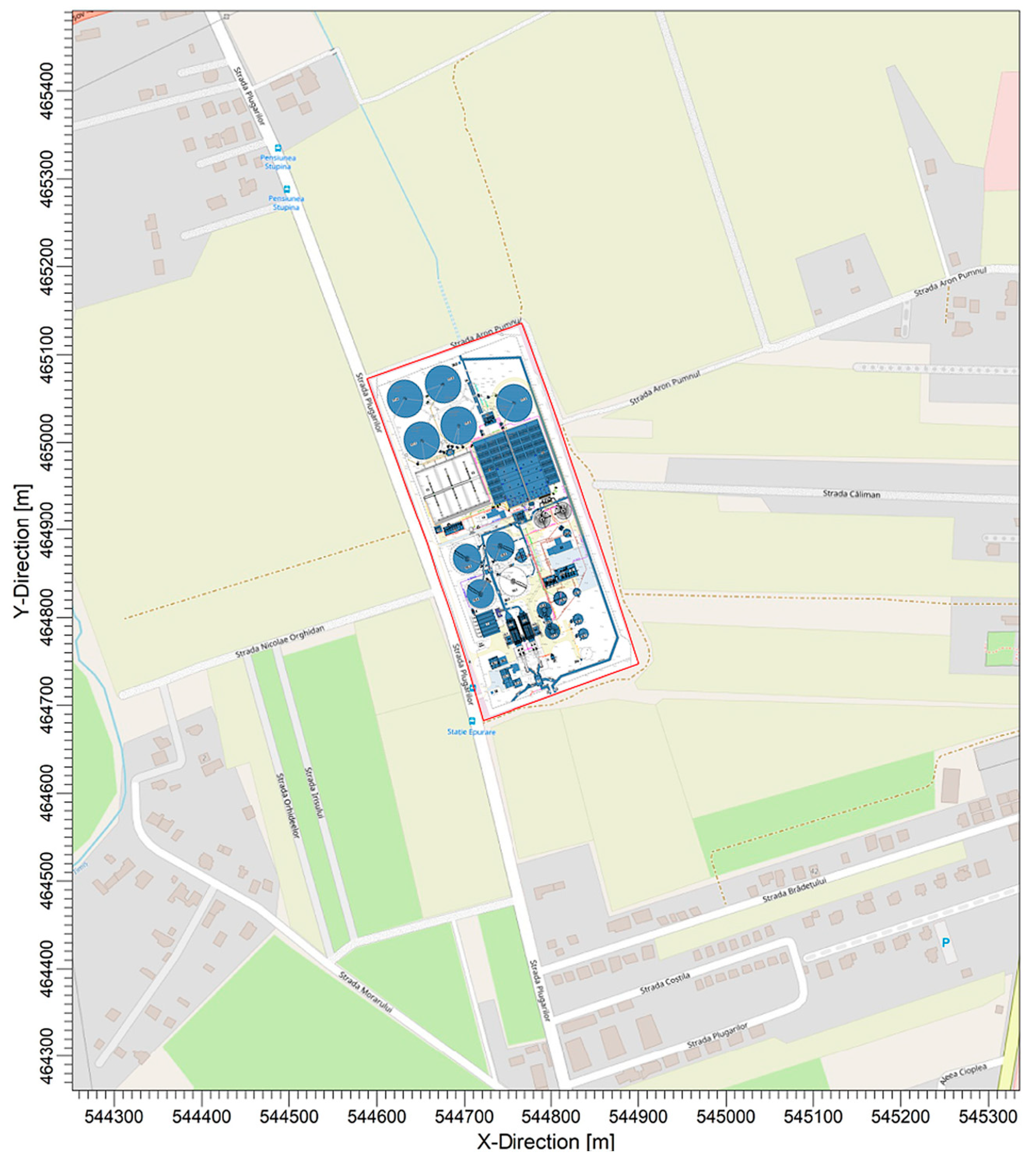
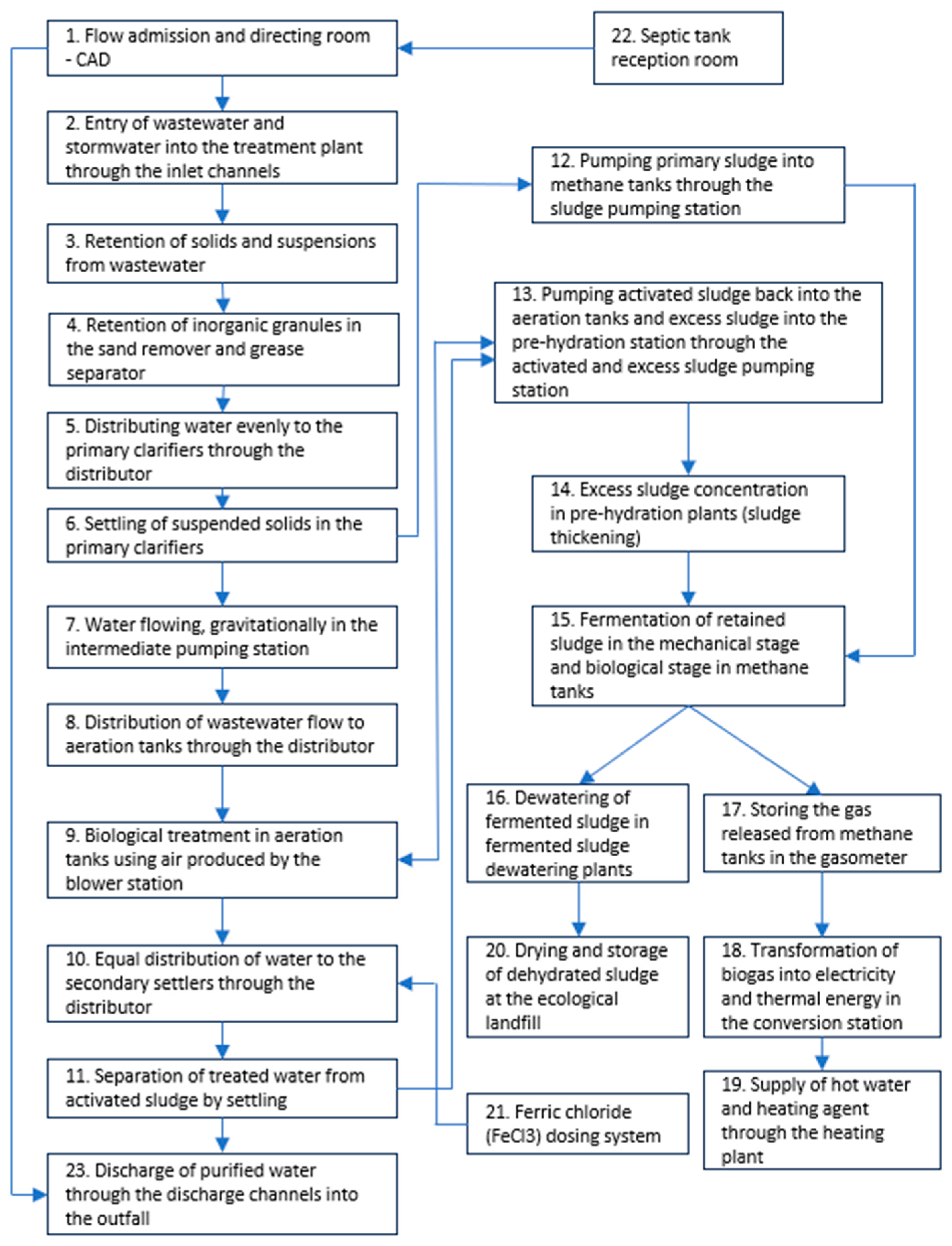
2.1. Description of the Wastewater Treatment Plant and Main Odor Sources

The WWTP is located on the upper terrace of the Olt River, northwest of the town, and it is outside the urban area region and about 300 m from the municipality’s residential zones (Figure 1). This facility operates as a mechanical–biological treatment plant, and it uses activated sludge and an integrated advanced treatment stage.
The WWTP was designed to process wastewater from an equivalent population of 500,000 individuals, with a current treatment capacity of 140,000 m3/d (including industrial wastewater). The WWTP performs biological secondary treatment (active sludge) and sludge stabilization by dehydration and anaerobic digestion.
The facility’s principal odor sources, including the wastewater and sludge lines, indicate that three technical processes, i.e., mechanical treatment, biological treatment, and sludge processing, are the main sources for the odors in the surrounding air.
The diffuse surface emission sources were represented by the emission surfaces of the following installations: sand remover/grease separator, primary decanters, primary sludge pumping tank, primary sludge gravity concentrator, primary and excess sludge mixing tank, fermented sludge buffer tank, activated sludge tank distribution chamber, activated sludge tanks, aeration tanks, and secondary decanters. The entire technological process that is applied to the sludge and wastewater is presented in Figure 2.
The contribution of emissions from other technological processes related to the WWTP was decided to be insignificant in terms of air pollution with odorous compounds and was not considered in the process of estimating the odor concentration in the surrounding air using mathematical modeling.

2.2. Odor Measurements

Odor emissions into the air were characterized by measuring the physical characteristics of each emission source, as well as the associated odor concentration. In contrast, for surface sources, the specific factors measured to estimate the emission rate are the emission surface and the air flow rate inside the sampling hood. During the sampling sessions on 27 and 29 May 2024, odor sampling and physical parameter measurements of the sources and gaseous effluents were performed [25].
One sample was taken from each sampling point from the WWTP unit sources using a wind tunnel-specific sampling hood with a surface area of 0.5 m2, which was placed on the sampling locations’ surfaces (Figure 3a).
The hood was equipped with two radial fans that ensure a constant volumetric flow for representative ventilation. The inlet fan draws the outside air through an orifice equipped with a replaceable activated carbon filter and directs it over the entire surface covered by the hood, capturing the released pollutants emitted by the surface source. At the same time, the air was extracted in the opposite corner by the second radial fan using another orifice with the same volumetric flow rate. The sample was taken through an orifice positioned in the cavity of the hood, where the neutral air mixes with the raw gas emitted by the source [33].
The technique involves collecting samples of the gaseous effluent released from the emission sources in containers made of inert materials, which are not contaminated with substances corresponding to the possible chemical components present in the sample gas. The odor concentration is then assessed using the dynamic olfactometry method. Samples from fixed emission sources were collected in specially certified Nalophan bags using 10 L vacuum equipment over a 30 min period, covering the entire area sources (Figure 3a).
Odor measurements were carried out using sensory determination with a dynamic olfactometer, which use the human nose as a detector (Figure 3b). This equipment is a high-accuracy diluter, and it is necessary for a group of four human assessors to conduct the odor evaluation, as has been applied in our previous studies [34].
Evaluators represent a group of people with an average response to the odor, and they are trained, selected, validated, and periodically checked to identify the presence of odor in the gas transmitted by the dynamic olfactometer. The validation/verification tests of the assessor use certified reference material, N-butanol, and the acceptability criteria are similar to the classical analytical methods [35].
The applied method involves panelists testing the odorous air at predefined dilutions. The EN 13725:2022 standard approach selects these panelists based on their average sensing capacity. The level of odor perception that the panelists reported is measured, and the results are used to figure out the stimulant’s odor concentration in ouE/m3 using the usual method [36].
The odor concentration, generally expressed as odor units relative to volume (ouE/m3), is numerically equal to the dilution factor of the sample required to reach the panel-specific perception threshold, which is the minimum concentration perceived by 50% of the population. According to EN 13725:2022, an odor unit (1 ouE/m3) is defined as “the amount of (a mixture of) odor substances present in a cubic metre of odor gas (under standard conditions) at the perception threshold of the assessor group”. In other words, at a concentration of 1 ouE/m3, 50% of the population can perceive an odor if exposed to an environment containing odorant mixture with this concentration [36].
Regarding the quality control of the results, the method used for odor concentration, using dynamic olfactometry, was verified in an International Interlaboratory Comparison Scheme organized by Olfasense GmbH, Kiel, Germany, in September 2023. In the test, a certified reference material (CRM), consisting of n-butanol in nitrogen with various unknown concentrations was used. The performance parameters verified was accuracy (Aod) and repeatability (r). The values obtained were compared with the values provided by the scheme organizer: Aod = 0.125 ≤ 0.217 and r = 0.083 ≤ 0.477. The limit of quantification, calculated from the olfactometer specifications, was 13.6 ouE/m3. Internal laboratory reproducibility was 12.51%, and uncertainty budget of the method was 46.85%.

2.3. Determination of Odor Emission Rate from Area Source

The specific odor emission rate (SOER) is similar to emission factors for other pollutants/chemical compounds in that they relate the quantity of a pollutant released into the atmosphere to a particular associated activity [31].
The specific flow of the surface source is expressed in m3/(m2h) and is determined by dividing the defined flow m3/h and multiplying it by the size of the entire surface m2 [28].
In this study, the emission from the diffuse area source was calculated using Formula (1).
SOER = Cod × Qair/Ahood,
where:
  • SOER is the specific odor emission rate in ouE/m2/s;
  • Qair is the airflow inside the hood (m3·s−1) (equal to 180 L/h);
  • Cod is the odor concentration in ouE/m3;
  • Ahood is the area of the wind tunnel in m2 (equal to 0.5 m2).
It is essential to note that the odor concentration of the sample withdrawn from the wind tunnel is proportional to the sweep air flow rate: the higher the latter, the greater the dilution for the emitted sample, resulting in lower odor concentrations. Experiments show that if the fan operates with sweep air flows of 50–500 L/h that do not interfere with surface emission, the odor concentration and sweep air flow remain constant [37].
The odor emission rate (OER) can be obtained as a product of the SOER and the total emitting surface (Asource) using Formula (2).
OER = SOER × Asource.

2.4. Model Description

Gaussian atmospheric dispersion models, such as the industrial source complex model AERMOD, have been utilized to evaluate pollution impacts in a variety of scenarios. Dispersion modeling is capable of predicting pollutant dispersion using emission data [38].
AERMOD View uses an atmospheric dispersion model based on the turbulence structure of the atmosphere layers and scaling concepts, including the treatment of multiple point sources at ground level or at altitude (AERMOD View software platform version 11.2.0.). It can be used for flat or complex terrain, rural or urban, and it includes algorithms for the effects that occur due to buildings. In the study, the Gaussian dispersion model was used for stable atmospheric conditions and the non-Gaussian models were used for unstable conditions. The simulation of dispersion in a complex terrain is achieved by procedures based on the separation of streamlines that allow pollutants to move over or around landforms, depending on the height of the pollutant plume and the stability conditions [39].
The mathematical modeling was performed under the following modeling conditions:
  • A Uniform Cartesian Grid was used to apply two receptor networks, with one on the entire surface of the dispersion map (6200 × 6200 m) and 32 points spaced 200 m apart, giving a total of 1024 receptors. The second network was applied centrally at the site level, covering 2450 × 2450 m and having 50 points spaced 50 m apart, giving a total of 2500 receptors for a uniform distribution of the iso–concentration curves at the level of the dispersion maps.
  • Topographic data processing was performed using the AERMAP terrain processor, which is included in the AERMOD software platform. The “flat terrain” option was used with a digital map in SRTM 30 format (Shuttle Radar Topography Mission) with the aim of creating digital terrain maps over almost the entire surface of the Earth with a resolution of 30 m.
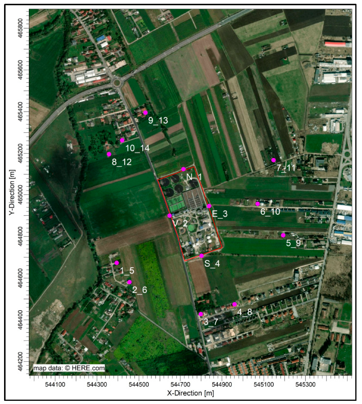
  • To draw attention to the odor concentrations estimated at the property’s edge and in populated areas close to the WWTP, 14 locations of sensitive Cartesian receptors were inserted in the model (4 at the property’s edge and 10 in populated areas), as shown in Table 1.
The spatial distribution of the introduced sensitive receptors is found in Figure 4.

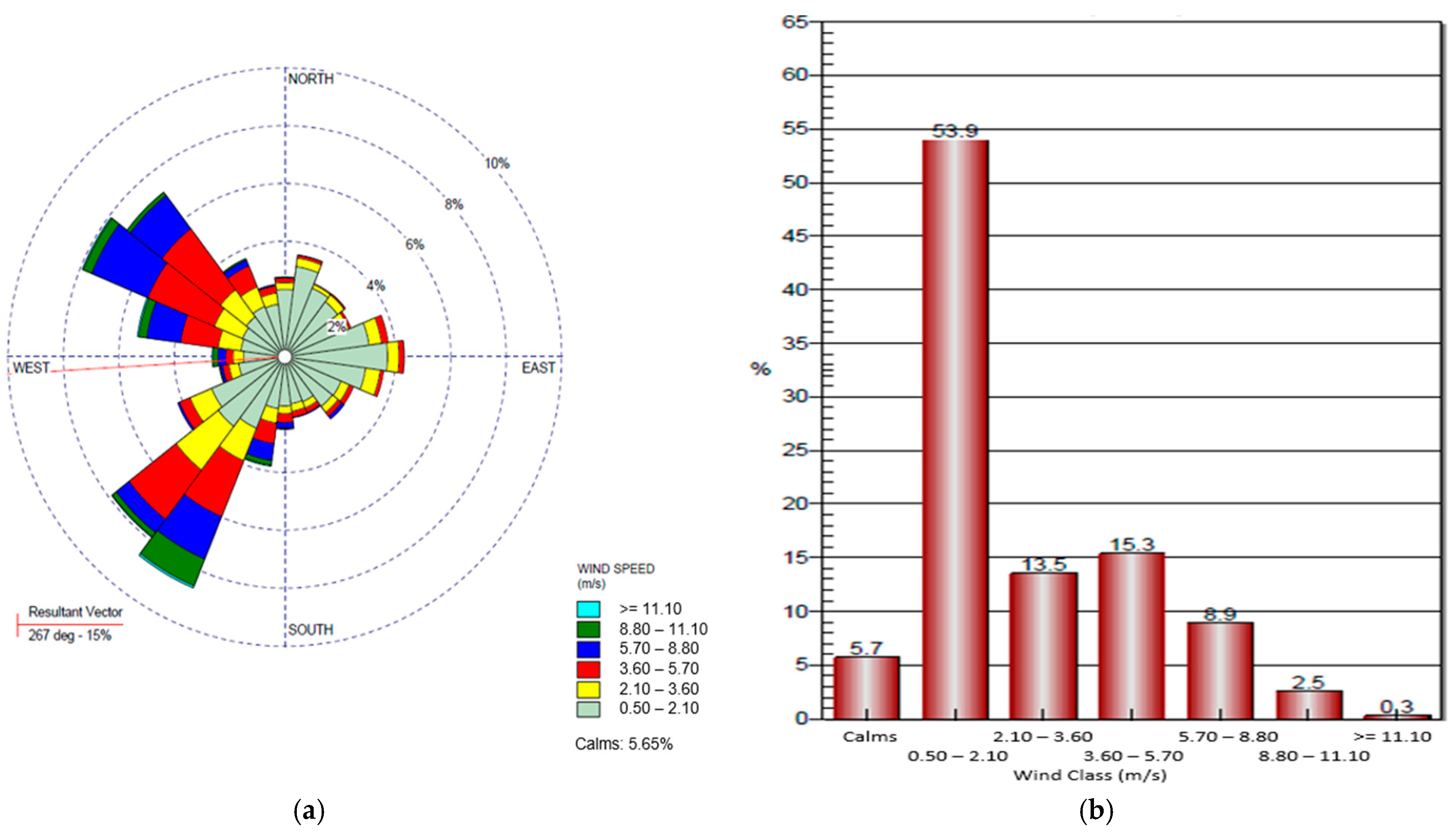
2.5. Meteorological Data Used

To perform the mathematical modeling of the odor dispersion in the atmospheric air, validated meteorological data were used, which were provided by the Romanian National Meteorological Administration, RNMA [40]. The data used were for the year 2023, and they were provided by the municipal meteorological station. The data characterized six meteorological parameters (temperature, pressure, humidity, cloudiness, wind speed, and direction) as hourly averages, according to the requirements of the dispersion program. The approximate distance of the weather station from the studied location is 4500 m. This proximity enables the collection of relatively accurate weather data, guaranteeing that the observed conditions accurately reflect the local environment.
The weather data were statistically processed with the AERMET View program to eliminate outliers and create a wind rose (Figure 5a), which represents the annual distribution of the wind direction in the area, and it is presented in a “blowing from” format. In general, a distribution of winds with dominant directions from the W-NW and SW was observed.
In this project, the upper air estimator was utilized as a preprocessing tool. This feature, which is a non-US EPA AERMET option, enables the generation of upper air data, and it is based only on hourly surface meteorological data. It provides an alternative to using actual upper air sounding data, allowing for more flexible and efficient processing when such direct measurements are unavailable [39]. During the data conversion process, the surface roughness, Bowen ratio, and albedo were specified by land use type, and it was divided into 12 sectors and selected as the annual average. The values of the surface used for processing meteorological data are presented in Table 2.
Regarding the frequency of winds, a strong presence of wind classes in the range of 0.5–2.1 m/s was observed throughout approximately 54% of the year, whereas the range of 2.1–3.6 m/s and 3.6–5.7 m/s, covering a smaller period, was observed throughout approximately 29% of the year (Figure 5b). Winds with higher intensity were present in a percentage of approximately 12% of the year.

2.6. Analyzed Parameters

To verify the toxicity of the air samples, the H2S, NH3, and VOCs levels were measured with three different pieces of equipment.
  • A Horiba APSA-370 for ambient H2S monitoring measured the SO2 converted H2S through an oxidation catalyst based on Ultra Violet Fluorescence. In order to reduce the measurement error by water concentration fluctuation in ambient conditions, the humidifier was set at the sample line. This enables long-term stability according to stabilizing catalytic reaction. The analyzer operates within a measurement range of 0 to 0.5 ppm, making it well suited for monitoring low concentrations of H2S in a variety of environments. It delivers high performance, with a repeatability of ±1.0% and linearity of ±1.0%, ensuring both precision and reliability throughout the entire measurement range. The measurement uncertainty is estimated at ±19%.
  • A Horiba APNA-370 automatic analyzer for ambient ammonia monitoring measured increased nitrogen oxide (NOx), which was found to have reacted through oxide catalyst treatment via the ammonia (NH3) concentration with the chemiluminescent (CLD) method. HORIBA’s original cross-flow modulation method ensures long-term stability and reliable measuring value with 5 ppb for minimum detectable sensitivity. This analyzer is capable of measuring NH3 within a range of 0 to 0.5 ppm, making it suitable for monitoring the low concentrations typically found in environmental and industrial settings. It offers excellent performance characteristics, with a repeatability of ±1.0% and linearity of ±1.0%, ensuring both consistent and accurate results across its full measurement range. The measurement uncertainty was estimated at ±18.3%.
  • The Thermo-FID model PT introduces a complete plug and play portable analyzer measuring Org.C components from a high range (ppm) to very low range (LEL). The portable unit includes gas bottle compartments and pressure regulators for both hydrogen and span gas. The instrument provides a built-in temperature regulator and mains supply for the standard external heated sample line (samples). It has a measurement range between 0 and 100 mg/Nm3. Calibration gases, specifically propane of a known concentration, are used to calibrate the analyzer. The measurement uncertainty was estimated at ±7.5%.

3. Results

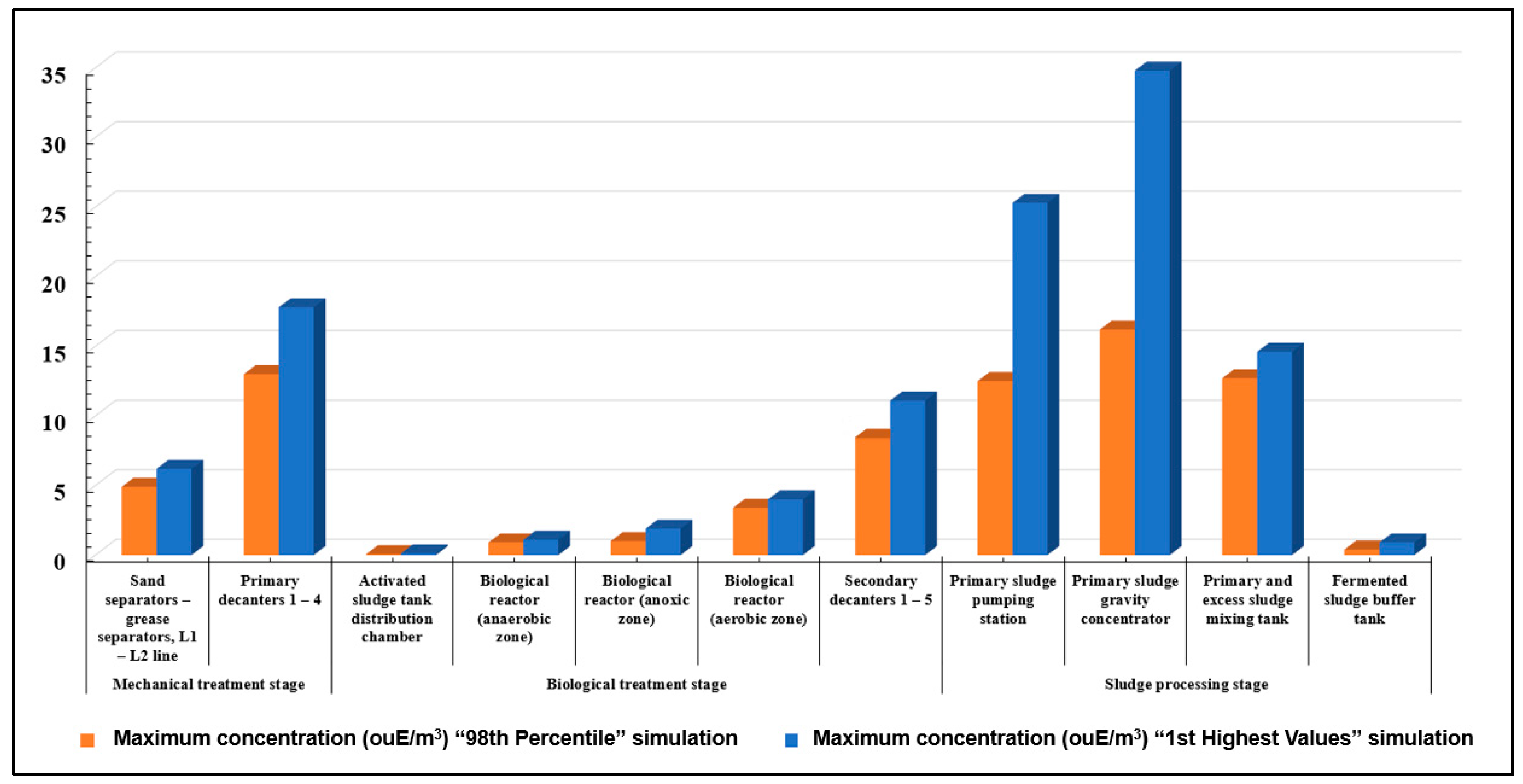
3.1. Results of the Odor Concentrations by Dynamic Olfactometry

The odor concentration was obtained using the dynamic olfactometry method, which measures the odor concentrations generated by on-site sources, as well as by mathematical modeling of the odor dispersion in the air, which was used to estimate the odor concentrations in the surrounding air.
The main odor sources found were the 13 surface emission sources, which were the tanks related to the technological processes of mechanical–biological treatment and sludge processing. These sources were surface emissions. The odor emission rate was determined in ouE/m2/s and used to estimate the total emission factor of the odor concentration from the area source.
Table 3 shows the results of olfactometric measurements, including the odor concentrations and emission rates. The results of the H2S, NH3, VOCs, and odor are reported with the uncertainty value associated. Odor concentrations in the samples ranged from 22 to 4171 ouE/m3, with a geometric mean of 159.6 ouE/m3. For the odor emission rate, we obtained a range from 0.16 to 34.76 ouE/m2/s, with a geometric mean of 1.54 ouE/m2/s.

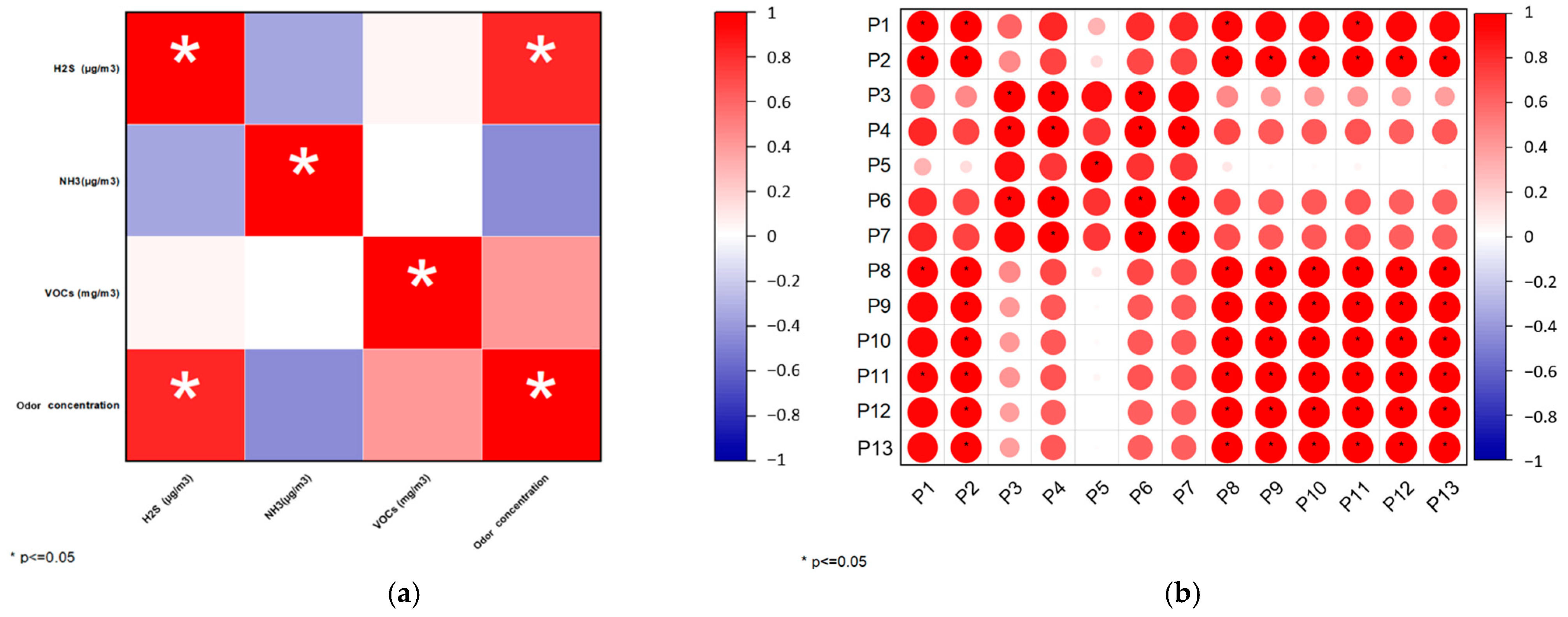
3.2. Pearson Correlation for the Analyzed Parameters

Figure 6a shows a correlation heatmap representing the relationships between the odor concentration and three key pollutants: hydrogen sulfide (H2S), ammonia (NH3), and volatile organic compounds (VOCs). The color scale ranges from −1 (strong negative correlation) to +1 (strong positive correlation), with red indicating positive correlations and blue indicating negative ones. Asterisks (*) denote statistically significant correlations with p-values < 0.05, suggesting strong evidence against randomness in the observed relationships. As shown in Figure 6a, there is a significant correlation between the odor concentration and the concentration of H2S (p ≤ 0.05). The VOC concentrations were also correlated significantly with the odor concentration, reinforcing their role as a major contributor to odor pollution.
Figure 6b illustrates the correlations between the different sampling sources (P1 to P13) regarding odor concentrations. The size and color intensity of the circles indicate the strength of the correlation. Red represents positive correlations, with deeper red and larger circles indicating stronger positive relationships. White or small faded circles imply weak or non-significant correlations. Blue (though not visibly present here) would indicate negative correlations.
Concerning the odor-generating sources, the correlations among them are illustrated in Figure 6b. The results obtained from Sources P1 (sand remover—grease separator, line 2) and P2 (primary decanters 1–3) were correlated with those from Sources P8–P11, which represent the areas where the sludge is stored, concentrated, mixed, and fermented. The results were also implicitly correlated with Sources P12 and P13 (which were non-operational at the time of sampling), with the p-value being ≤ 0.05.

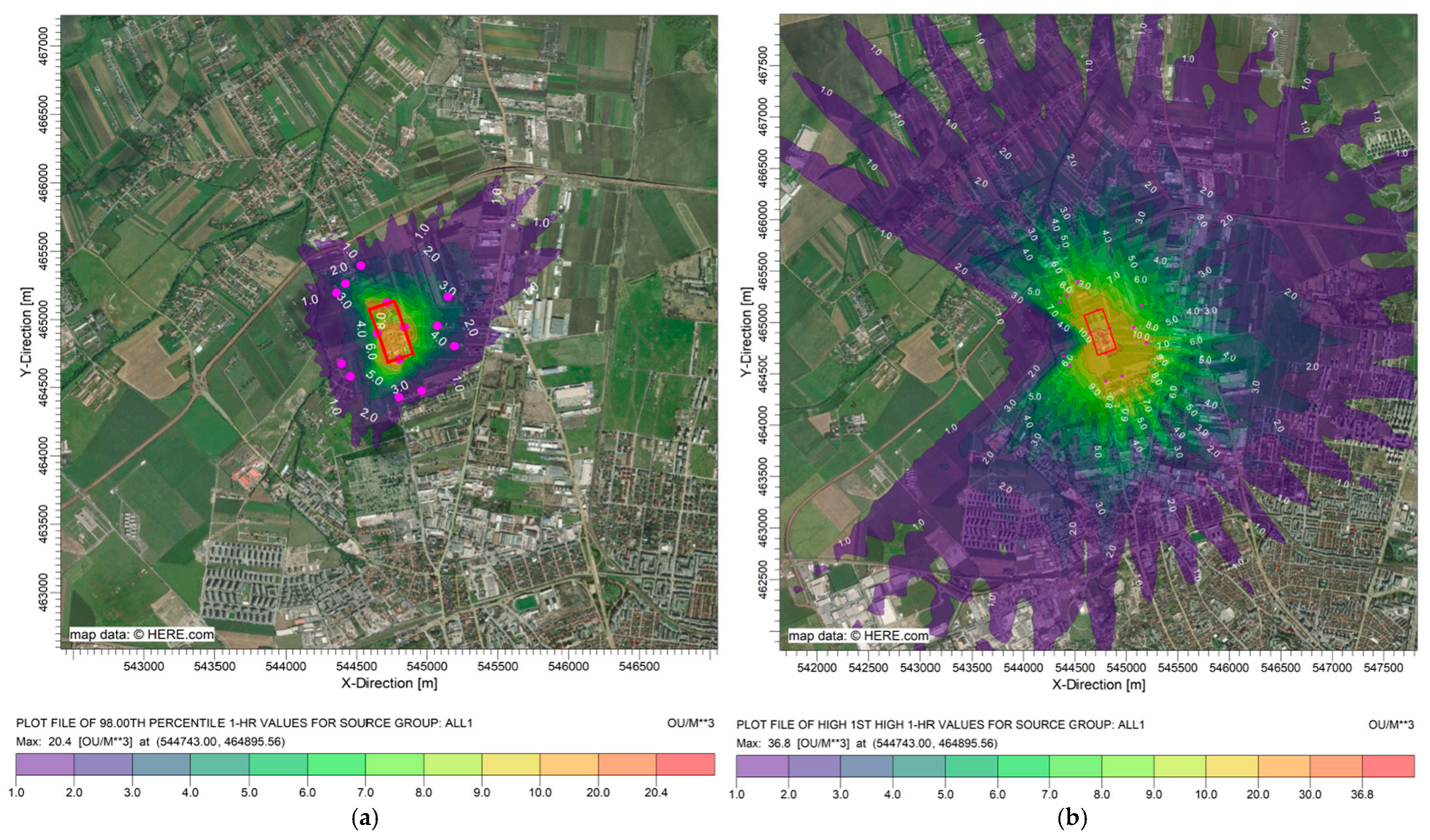
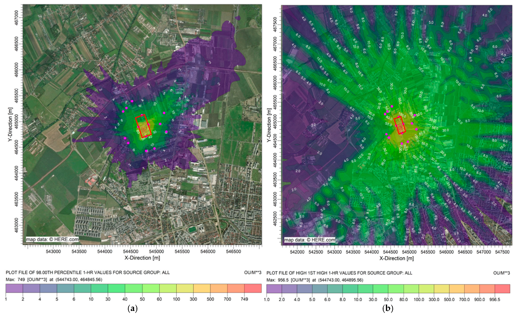
3.3. Results of the Odor Concentrations by Mathematical Modeling in the Surrounding Air

In order to estimate the odor concentration in the ambient air on the site and in the areas surrounding the WWTPs, two simulations with two mathematical modeling were performed using the 98th percentile function. The objective was to identify the level of the odor pollution generated by diffuse area sources on the site and in the surrounding area in 98% of a year, or over 8585 h under prevailing meteorological conditions specific to an entire year, apart from the most unfavorable dispersion conditions (1st highest value). These values represent an hourly average and are unique for each receptor. Two other mathematical models were constructed for the remaining 175 h of the year (2%). In this situation, it was found that the concentrations may reach higher values, largely due to meteorological conditions that are unfavorable to dispersion. This situation corresponds to the most unfavorable weather conditions for odor dispersion in the surrounding air, also known as the worst-case scenario.
Type A simulations were performed with the 1st highest value and 98th percentile functions for all diffuse area emission sources. The dispersion maps for this type of simulation includes the total contribution of all the diffuse area sources that were identified on the site of the WWTP under normal operating conditions, as shown in Figure 7a,b.
Type B simulations were performed with the 1st highest value and 98th percentile functions for all diffuse surface emission sources. The dispersion map for this type of simulation includes the total contribution of the diffuse area sources that were identified on the site of the WWTP with the grease collection system of the de-sanding/grease separation Unit Line 1 and the sludge collection system of the primary settling Decanter 4 out of operation, i.e., a situation that may be encountered at the time of sampling, as shown in Figure 8a,b.
Under these conditions, the following data were taken into account for the interpretation of the results, which were obtained through mathematical modeling:
  • The concentration of 1 ouE/m3 was considered as the minimum odor concentration perceived by 50% of the population, although only a part of the population showed a biological response at this concentration.
  • The limit values established by some European countries for residential areas are located in the range of 2–7 ouE/m3, and these are accompanied by a maximum number of hours per year when these limits can be exceeded or the 98th percentile value is applied.
  • The range of 5 ouE/m3 to 10 ouE/m3 is where olfactory discomfort occurs.
The Type A simulation within the 98th percentile function is presented in Figure 7a for all emission sources under normal operating conditions, and it shows a maximum concentration of 20.4 ouE/m3, which was recorded on the site, over 98% of a one-year period. The odor plume presents a reduced shape compared to the 1st highest values function, with halved iso–concentration curve values and a trend toward the east.
At the boundary of the WWTP, the highest value of the odor concentration was 12.48 ouE/m3 at Point (S_4), which is located in the southern part of the site (Table 4). At the level of the sensitive receptors located outside the site, the maximum concentration was at Point (6_10), which is east of the WWTP, and it had a concentration value of 4.91 ouE/m3.
The simulation in Figure 7b shows a maximum concentration of 36.8 ouE/m3 in the southern area of the site under the most unfavorable meteorological dispersion conditions for the entire year. At the site boundary, the highest value of the odor concentration was 20.17 ouE/m3 in the same point (S_4) located in the southern part of the site. The concentrations gradually decreased in the direction of the odor plume, reaching values between 2–1 ouE/m3 at distances greater than 1000 m outside the site. The highest values encountered at the level of sensitive receptors were 13.16 ouE/m3 at Point (4_8) and 12.20 ouE/m3 at Point (3_7); the values for the remaining points outside the site, where the sensitive receptors were introduced, were in the range of 4–9.8 ouE/m3.
The Type B simulation presented in Figure 8a for all emission sources modeled the grease collection system of the de-sanding/grease separation Unit Line 1 and sludge collection system of the primary settling Decanter 4 not working, and this modeling showed a maximum concentration of 749 ouE/m3, which was recorded on the site, over 98% of the one-year period. The odor plume presented an increased shape compared to the Type A simulation, with halved iso–concentration curve values and a trend toward the northeast.
At the boundary of the WWTP, the highest value of the odor concentration was 174.8 ouE/m3 at Point (E_3), which is located in the eastern part of the site. At the level of sensitive receptors located outside the site, within the 98th percentile simulation, the maximum concentration was at Point (6_10), which is east of the WWTP, and it had a concentration value of 18.63 ouE/m3.
The simulation, as presented in Figure 8b, under the most unfavorable meteorological dispersion conditions for the entire year showed a maximum concentration of 956.5 ouE/m3 in the central area of the site. At the site boundary, the highest value of the odor concentration was 407.6 ouE/m3 in the same Point (E_3), which is located in the southern part of the site. The odor plume disperses in all directions, mainly to the west, due to the prevailing easterly wind direction. In the directions of the plume, the concentrations gradually decrease, reaching values between 2–1 ouE/m3 after distances of over 3000 m.
The highest values encountered at the level of sensitive receptors for this simulation was 140.6 ouE/m3 at Point (4_8) and 126 ouE/m3 at Point (6_10); the values for the remaining points outside the site, where sensitive receptors were introduced, were in the range of 20–117 ouE/m3 (Table 4).
In Table 4, the odor concentrations for both the simulation with the 98th percentile and 1st highest values functions at the level of sensitive receptors are presented.
In order to identify the sources with the greatest influence on the level of odorous air pollution on the site and in its vicinity, especially in areas where homes are located, all of the sources were analyzed and modeled individually for the two distinct simulations using the “98th Percentile” and “1st Highest Values” functions. The results obtained through mathematical modeling in these conditions were specific to each source and can be found in Figure 9.

3.4. Result of the Odor Concentrations on the Environmental Air

The results obtained for the odor concentrations in the ambient air are presented in Table 5. The highest value, 23 ouE/m3, was recorded at Point 8_12, which is northwest, in June 2024. All other measured values were either below the method’s determination limit or close to this threshold.

4. Discussion

The obtained values of the odor concentrations at the level of the area source in the investigated WWTP (22–4171 ouE/m3) were lower than those reported in other studies, such as, for example, in the Izmir WWTP (131–16,384 ouE/m3) [15].
The highest contribution to odor pollution was observed when the primary settling Decanter 4 was out of service. In this scenario, the source emitted an odor concentration of 4171 ouE/m3, with an emission rate of 34.76 ouE/m2/s over a surface area of 887 m2. In the Type B simulation, which represents this malfunction scenario, significant odor levels were recorded both on the site of the treatment plant and in the surrounding areas. According to the “1st Highest Values” function, the maximum concentration reached 957 ouE/m3, (Figure 8b) while the “98th Percentile” function indicated a maximum concentration of 749 ouE/m3 (Figure 8a). Although this scenario does not reflect the normal operating conditions of a wastewater treatment plant, such situations are not uncommon and highlight the potential impact of equipment failures on odor emissions. The Pearson correlation confirmed that H2S and VOCs are the most influential compounds contributing to odor emissions in the wastewater treatment environment, while NH3 plays a more variable or indirect role (Figure 6a). These findings help guide targeted monitoring and mitigation strategies, prioritizing compounds with the greatest impact on odor levels.
In the normal conditions of WWTP functionality, the Type A simulation showed that the highest contribution to odor pollution came from the sludge processing stage, particularly from the primary sludge gravity concentrator with an emitted concentration of 1166 ouE/m3 with an emission rate of 9.27 ouE/m2/s over a surface area of 227 m2. To reduce the odor emissions from this type of source—which is among the most significant contributors to odor pollution—installations can be implemented to capture and filter the gases released during the sludge purification process.
The literature indicates a general range of 3 ouE/m3 to 5 ouE/m3 for concentrations detected by the majority of the population and a range of 5 ouE/m3 to 10 ouE/m3 for concentrations leading to a state of discomfort [20]. These ranges are not generally valid and depend on a multitude of factors, such as the sensitivity of each person, the character and intensity of the odor, the frequency, the location, etc. [41].
As a rule, interpreting the results of studies assessing air quality through mathematical modeling of the dispersion of pollutants in the air involves reporting the results obtained through modeling the limit values that are in force in the environmental regulations for ambient air quality. According to the Romanian legislation at the moment, no limit for the concentration of odor in the air has been set [42]. The only Romanian Standard that includes data regarding odor levels in protected areas is STAS 12574/87 [43]. In this standard, a definition of strongly odorous substances is presented: “emissions of strongly odorous substances exceed the maximum permitted concentrations when in the impact area their unpleasant and persistent odor is detectable” [43].
At the European level, there is no unified approach to odor regulations; some member states have, in various forms, set limit values for odor concentrations in air in their national legislation, but the vast majority do not have such limits. Most of these limits are between 2 and 7 ouE/m3 in the residential areas of countries like Italy, France, Belgium, Denmark, and the Netherlands [20]. They are usually accompanied by a maximum number of hours per year when these limits can be exceeded (usually 175) or the 98th percentile value. This way, when mathematical modeling studies of dispersion are performed, the highest estimated values are not interpreted because they are exceptions caused by bad or extreme weather (1st highest values) [44].
Efficient financial planning ensures that wastewater treatment plants can run smoothly, satisfy regulatory requirements, and continue to serve the community. Wastewater treatment plants, in turn, serve an important role in preserving public health and the environment by treating and purifying water before it is returned to natural water sources. Proper funding and management in all sectors are critical to long-term success and environmental conservation. Conservation efforts help maintain the ecological balance and support sustainable development initiatives within the community. By investing in innovative technologies and infrastructure improvements, wastewater treatment facilities can enhance their efficiency and reduce their environmental footprint, ultimately benefiting both residents and the ecosystem [45].

5. Conclusions

This study demonstrates the substantial influence of wastewater treatment plant (WWTP) operations on local air quality, particularly regarding the emission of odorous and potentially harmful substances, such as hydrogen sulfide (H2S), ammonia (NH3), and volatile organic compounds (VOCs). Through mathematical dispersion modeling using the AERMOD View platform, two distinct operational scenarios were analyzed to estimate odor concentrations under unfavorable meteorological conditions.
Results indicate that, under normal operating conditions, odor concentrations remain within a relatively low and controlled range. However, in the event of equipment failures—such as the shutdown of the grease collection system and primary sludge decanter—odor levels can escalate sharply, posing a significant nuisance and potential health concern for nearby residents.
These findings underscore the critical need for continuous monitoring, rigorous maintenance protocols, and compliance with environmental regulations. Furthermore, transparent communication and active engagement with stakeholders are essential for building public trust and ensuring effective odor management. By prioritizing preventative measures and investing in system reliability, WWTP operators can significantly mitigate emission risks and contribute to a healthier environment for surrounding communities.
The methodology applied differs from most odor studies in the literature, where ambient air monitoring is used, when compared to direct sampling from the surface emission source. This study provides a substantial advancement in sampling techniques via using a wind tunnel to estimate the concentrations in diverse scenarios through mathematical modeling of the odor dispersion in the surrounding air utilizing the AERMOD View software platform. This comprehensive approach incorporates emission data from the sampled areas, along with validated meteorological and topographical data specific to the region. This approach will allow one to predict how different variables, such as wind speed and direction, affect the spread of odors and pollutants.
The obtained results highlight the variability in pollutant concentrations depending on the modeling approach used. Furthermore, they emphasize the importance of ongoing monitoring and assessment to ensure compliance with environmental standards and protect sensitive receptors in the surrounding area. By comparing the results from different simulation methods, researchers can better understand the potential impacts of pollutants and make informed decisions regarding mitigation strategies. This comprehensive approach not only aids in regulatory compliance, but also fosters community trust in environmental management practices. Trust in environmental management practices is crucial for fostering collaboration between regulatory agencies and local communities. Engaging stakeholders in discussions about pollutant impacts and mitigation efforts can lead to more effective strategies that benefit both public health and the environment.

Author Contributions

Conceptualization, C.C. and G.O.G.; methodology, C.C. and G.O.G.; software, C.C.; validation, C.M., A.M.D., and S.M.C.; formal analysis, V.D. and G.T.; investigation, C.C. and A.C.; data curation, S.M.C.; writing—original draft preparation, C.C. and G.G.V.; writing—review and editing, C.C. and G.G.V.; visualization, G.G.V., C.C., and C.M.; supervision, S.M.C.; project administration, S.M.C.; funding acquisition, G.G.V. and S.M.C. All authors have read and agreed to the published version of the manuscript.

Funding

This research was financially supported by the National Research and Development Institute for Industrial Ecology–ECOIND. Odor measurements conducted at the Municipal Wastewater Treatment Plant were funded by the plant administration.

Institutional Review Board Statement

Not applicable.

Informed Consent Statement

Informed consent was obtained from all subjects involved in the study. The research was conducted in accordance with established ethical guidelines, ensuring that participants were fully informed about the procedures and any potential risks. This approach protected their rights and contributed to the reliability and integrity of the study’s findings.

Data Availability Statement

Data are contained within the article.

Acknowledgments

We acknowledge the support of the following odor assessors: Elena Dicu, Lavinia Moise, Veronica Iordache, and Cornel Dan. We are grateful for their involvement in the odor determinations.

Conflicts of Interest

The authors declare no conflicts of interest.

References

  1. Munsif, R.; Zubair, M.; Aziz, A.; Nadeem Zafar, M. Industrial Air Emission Pollution: Potential Sources and Sustainable Mitigation. In Environmental Emissions, 1st ed.; Viskup, R., Ed.; IntechOpen Limited: London, UK, 2021; pp. 1–13. [Google Scholar] [CrossRef]
  2. Zhou, P.; Sun, S.; Chen, T.; Pan, Y.; Xu, W.; Zhang, H. Impacts of Social Inequality, Air Pollution, Rural–Urban Divides, and Insufficient Green Space on Residents’ Health in China: Insight from Chinese General Social Survey Data Analysis. Int. J. Environ. Res. Public Health 2022, 19, 14225. [Google Scholar] [CrossRef] [PubMed]
  3. Gutiérrez, M.C.; Hernández-Ceballos, M.A.; Márquez, P.; Chica, A.F.; Martín, M.A. Identification and simulation of atmospheric dispersion patterns of odour and VOCs generated by a waste treatment plant. Atmos. Pollut. Res. 2023, 14, 101636. [Google Scholar] [CrossRef]
  4. Agus, E.; Zhang, L.; Sedlak, D.L. A framework for identifying characteristic odor compounds in municipal wastewater effluent. Water Res. 2012, 46, 5970–5980. [Google Scholar] [CrossRef]
  5. Abe, K.C.; Dos Santos, G.M.S.; Coêlho, M.S.Z.S.; Miraglia, S.G.E.K. PM 10 exposure and cardiorespiratory mortality—Estimating the effects and economic losses in São Paulo, Brazil. Aerosol Air Qual. Res. 2018, 18, 3127–3133. [Google Scholar] [CrossRef]
  6. Vítězová, M.; Vítěz, T.; Mlejnková, H.; Lošák, T. Microbial contamination of the air at the wastewater treatment plant. Acta Univ. Agric. Silvic. Mendel. Brun. 2012, LX, 233–240. [Google Scholar] [CrossRef]
  7. Ren, B.; Zhao, Y.; Lyczko, N.; Nzihou, A. Current Status and Outlook of Odor Removal Technologies in Wastewater Treatment Plant. Waste Biomass Valor. 2019, 10, 1443–1458. [Google Scholar] [CrossRef]
  8. Teixeira, J.V.; Miranda, S.; Monteiro, R.A.R.; Lopes, F.V.S.; Madureira, J.; Silva, G.V.; Pestana, N.; Pinto, E.; Vilar, V.J.P.; Boaventura, R.A.R. Assessment of indoor airborne contamination in a wastewater treatment plant. Environ. Monit. Assess. 2013, 185, 59–72. [Google Scholar] [CrossRef]
  9. Márquez, P.; Muñoz-Serrano, E.; Gutiérrez, M.C.; Siles, J.A.; Martín, M.A. Odour impact simulation of a large urban wastewater treatment plant through the numerical solution of a Eulerian model. J. Environ. Manag. 2024, 372, 123327. [Google Scholar] [CrossRef]
  10. Widiana, D.R.; Wang, Y.F.; You, S.J.; Yang, H.H.; Wang, L.C.; Tsai, J.H.; Chen, H.M. Air pollution profiles and health risk assessment of ambient volatile organic compounds above a municipal wastewater treatment plant, Taiwan. Aerosol Air Qual. Res. 2019, 19, 375–382. [Google Scholar] [CrossRef]
  11. Saleh, I.A.; Mohammed, A.M.F. Contour maps of Air Pollutants and their Health Risk Assessment in Abu-Rawash Wastewater Treatment Plant, Egypt. Egypt J. Chem. 2023, 66, 319–330. [Google Scholar] [CrossRef]
  12. Rolewicz-Kalińska, A.; Lelicińska-Serafin, K.; Manczarski, P. Volatile organic compounds, ammonia and hydrogen sulphide removal using a two-stage membrane biofiltration process. Chem. Eng. Res. Des. 2021, 165, 69–80. [Google Scholar] [CrossRef]
  13. Godayol, A.; Alonso, M.; Besalú, E.; Sanchez, J.M.; Anticó, E. Odour-causing organic compounds in wastewater treatment plants: Evaluation of headspace solid-phase microextraction as a concentration technique. J. Chromatogr. A 2011, 1218, 4863–4868. [Google Scholar] [CrossRef]
  14. Carrera-Chapela, F.; Donoso-Bravo, A.; Souto, J.A.; Ruiz-Filippi, G. Modeling the odor generation in WWTP: An integrated approach review. Water Air Soil Pollut. 2014, 225, 1–15. [Google Scholar] [CrossRef]
  15. Dinçer, F.; Dinçer, F.K.; Sarı, D.; Ceylan, Ö.; Ercan, Ö. Dispersion modeling and air quality measurements to evaluate the odor impact of a wastewater treatment plant in İzmir. Atmos. Pollut. Res. 2020, 11, 2119–2125. [Google Scholar] [CrossRef]
  16. Gonzales, D.; Colon, J.; Sanchez, A.; Gabriel, D. Multipoint characterization of the emission of odour, volatile organic compounds and greenhouse gases from a full-scale membrane-based municipal WWTP. J. Environ. Manag. 2022, 313, 115002. [Google Scholar] [CrossRef]
  17. Jonca, J.; Miller, U.; Wrobel, M.; Bezyk, Y.; Wloka, A.; Janicka, A.; Sowka, I. A comprehensive approach to assess odorous air quality of a selected wastewater treatment plant: Preliminary study. Desalin. Water Treat. 2025, 322, 101168. [Google Scholar] [CrossRef]
  18. Liao, Z.; Gao, T.; Li, P.; Zheng, T.; Li, L.; Li, C.; Wang, W.; Wang, Y.; Liu, J. Diffusion behavior and environmental impact of odorants and TVOCs detected in a wastewater treatment plant for collaborative leachate treatment in Northwest China. Chemosphere 2024, 366, 143561. [Google Scholar] [CrossRef]
  19. Brancher, M.; Griffiths, K.D.; Franco, D.; de Melo Lisboa, H. A review of odour impact criteria in selected countries around the world. Chemosphere 2017, 168, 1531–1570. [Google Scholar] [CrossRef]
  20. Canadian Environmental Protection Act. Guidance Manual for the Wastewater Sector; National Pollutant Release Inventory; Environment Canada: Gatineau, QC, Canada, 2003. [Google Scholar]
  21. Scotto Di Perta, E.; Fiorentino, N.; Carozzi, M.; Cervelli, E.; Pindozzi, S. A Review of Chamber and Micrometeorological Methods to Quantify NH3 Emissions from Fertilizers Field Application. Int. J. Agron. 2020, 2020, 1–16. [Google Scholar] [CrossRef]
  22. Loubet, B.; Cellier, P.; Flura, D.; Génermont, S. An Evaluation of the Wind-tunnel Technique for Estimating Ammonia Volatilization from Land: Part 1. Analysis and Improvement of Accuracy. J. Agric. Eng. Res. 1999, 72, 71–81. [Google Scholar] [CrossRef]
  23. Hafner, S.D.; Kamp, J.N.; Pedersen, J. Experimental and model-based comparison of wind tunnel and inverse dispersion model measurement of ammonia emission from field-applied animal slurry. Agric. For. Meteorol. 2024, 344, 109790. [Google Scholar] [CrossRef]
  24. Lucernoni, F.; Capelli, L.; Busini, V.; Sironi, S. A model to relate wind tunnel measurements to open field odorant emissions from liquid area sources. Atmos. Environ. 2017, 157, 10–17. [Google Scholar] [CrossRef]
  25. Capelli, L.; Sironi, S.; del Rosso, R. Odor sampling: Techniques and strategies for the estimation of odor emission rates from different source types. Sensors 2013, 13, 938–955. [Google Scholar] [CrossRef]
  26. Moreno-Silva, C.; Calvo, D.C.; Torres, N.; Ayala, L.; Gaitan, M.; Gonzales, L.; Rincon, P.; Rodrigues Susa, M. Hydrogen sulphide emissions and dispersion modelling from a wastewater reservoir using flux chamber measurements and AERMOD® simulations. Atmos. Environ. 2020, 224, 117263. [Google Scholar] [CrossRef]
  27. Prata, A.A., Jr.; Santos, J.M.; Beghini, S.P.; Fernandes, I.F.; Vom Marttens, L.L.C.; Pereira Neto, L.I.; Martians, R.S.; Reis, N.C., Jr.; Stuetz, R.M. Dynamic flux chamber measurements of hydrogen sulfide emission rate from a quiescent surface—A computational evaluation. Chemosphere 2016, 146, 426–434. [Google Scholar] [CrossRef]
  28. Lucernoni, F.; Tapparo, F.; Capelli, L.; Sironi, S. Evaluation of an Odour Emission Factor (OEF) to estimate odour emissions from landfill surfaces. Atmos. Environ. 2016, 144, 87–99. [Google Scholar] [CrossRef]
  29. McCollough, M.R.; Pedersen, J.; Nyord, T.; Sørensen, P.; Melander, B. Ammonia Emissions, Exposed Surface Area, and Crop and Weed Responses Resulting from Three Post-Emergence Slurry Application Strategies in Cereals. Agronomy 2022, 12, 2441. [Google Scholar] [CrossRef]
  30. Pedersen, J.M.; Feilberg, A.; Kamp, J.N.; Hafner, S.; Nyord, T. Ammonia emission measurement with an online wind tunnel system for evaluation of manure application techniques. Atmos. Environ. 2020, 230, 117562. [Google Scholar] [CrossRef]
  31. Nicell, J.; Henshaw, P. Odor impact assessments based on dose-response relationships and spatial analyses of population response. Water Pract. 2006, 1, 1–14. [Google Scholar] [CrossRef]
  32. Vieira de Melo, A.M.; Santos, J.M.; Mavroidis, I.; Reis Junior, N.C. Modelling of odour dispersion around a pig farm building complex using AERMOD and CALPUFF. Comparison with wind tunnel results. Build. Environ. 2012, 56, 8–20. [Google Scholar] [CrossRef]
  33. Odournet Product Catalogue. 2015. Available online: https://www.odournet.com/wp-content/uploads/2015/07/Odournet-Product-Catalogue-2015.pdf (accessed on 25 June 2024).
  34. Constantin, C.; Popa, G.O.; Calinescu, S.; Tanase, G. Determination of odour emission rates emitted by active area sources and dispersion of odour concentration in the surrounding air. Rom. J. Ecol. Environ. Chem. 2023, 5, 117–127. [Google Scholar] [CrossRef]
  35. Hawko, C.; Verriele, M.; Hucker, N.; Crunaire, S.; Leger, C.; Logoge, N.; Savary, G. A review of environmental odor quantification and qualification methods: The question of objectivity in sensory analysis. Sci. Total Environ. 2021, 795, 148862. [Google Scholar] [CrossRef] [PubMed]
  36. EN 13725:2022; Emissions from Stationary Sources. Determination of Odor Concentration by Dynamic Olfactometry and Odor Emission Rate. European Committee for Standardization (CEN): Brussels, Belgium, 2022.
  37. Sironi, S.; Capelli, L.; Céntola, P.; Del Rosso, R.; Pierucci, S. Odour impact assessment by means of dynamic olfactometry, dispersion modelling and social participation. Atmos. Environ. 2010, 44, 354–360. [Google Scholar] [CrossRef]
  38. Lakes Software. Available online: https://www.weblakes.com/software/air-dispersion/aermod-view/ (accessed on 25 June 2024).
  39. User’s Guide for the AMS/EPA Regulatory Model (AERMOD); U.S. Environmental Protection Agency: Washington, DC, USA, 2024. Available online: https://nepis.epa.gov/Exe/ZyPURL.cgi?Dockey=P100XN2J.TXT (accessed on 26 June 2024).
  40. Romanian National Meteorological Administration. Available online: https://www.meteoromania.ro/ (accessed on 31 July 2024). (In Romanian).
  41. Conti, C.; Guarino, M.; Bacenetti, J. Measurements techniques and models to assess odor annoyance: A review. Environ. Int. 2020, 134, 105261. [Google Scholar] [CrossRef]
  42. Law No. 123/2020, Odor Law Regarding the Amendment and Completion of Government Emergency Ordinance No. 195/2005 on Environmental Protection. Available online: https://legislatie.just.ro/Public/DetaliiDocument/227780 (accessed on 15 October 2024). (In Romanian).
  43. STAS 12574/87. Air Quality. Air from Protected Areas. Quality Conditions. Available online: https://magazin.asro.ro/ro/standard/19048 (accessed on 15 October 2024). (In Romanian).
  44. Bokowa, A.; Diaz, C.; Koziel, J.A.; McGinley, M.; Barclay, J.; Schauberger, G.; Guillot, J.M.; Sneath, R.; Capelli, L.; Zorich, V.; et al. Summary and Evaluation of the Odour Regulations Worldwide. Atmosphere 2021, 12, 206. [Google Scholar] [CrossRef]
  45. Stefan-Duicu, V.M.; Stefan-Duicu, A. Global Analysis of the Financial Analyst’s Job within a Company. Procedia Econ. Financ. 2015, 26, 261–267. [Google Scholar] [CrossRef]
Figure 1. Location of the WWTP in the studied municipality.
Atmosphere 16 00577 g001
Figure 2. The technological process applied in the selected WWTP.
Atmosphere 16 00577 g002
Figure 3. (a) Wind tunnel-specific sampling hood with a surface area of 0.5 m2. (b) The TO8 olfactometer used in the experimental part.
Atmosphere 16 00577 g003
Figure 4. The locations of the points where the sensitive receptors were introduced.
Atmosphere 16 00577 g004
Figure 5. (a) The wind roses in the selected municipality—blowing from format. (b) The frequency of the winds.
Atmosphere 16 00577 g005
Figure 6. (a) The correlations between the odor concentration and the H2S, NH3, and VOC results (p-value). (b) The correlations between the sampling sources regarding odor concentrations (p-value).
Atmosphere 16 00577 g006
Figure 7. (a) The hourly average of the highest values over 98% of a one-year period for all emission sources represents the 98th percentile for type A simulation. (b) The hourly average of the highest values over 2% of the year for all emission sources represents the 1st highest values for type A simulation.
Atmosphere 16 00577 g007
Figure 8. (a) The hourly average of the highest values over 98% of a one-year period for all emission sources represents the 98th percentile for type B simulation. (b) The hourly average of the highest values over 2% of the year for all emission sources represents the 1st highest values for type B simulation.
Atmosphere 16 00577 g008
Figure 9. The results of the odor concentrations for each odor source identified on the WWTP site for the two types of simulations: 1st highest values and 98th percentile.
Atmosphere 16 00577 g009
Table 1. The sensitive receptor code and relative position to the investigated site.
Identification CodeLocationIdentification CodeLocationIdentification CodeLocation
N_1Northern limit of the WWTP site1_5Southwest6_10East
V_2Western limit of the WWTP site2_6Southwest7_11East
E_3Eastern limit of the WWTP site3_7South8_12Northwest
S_4Southern limit of the WWTP site4_8South9_13North
Table 2. The values of the surface data based on the proximity from the meteorological station.
Specify SectorsAlbedoBowen RatioSurface RoughnessLand Type
1 (0–30°)0.28 0.75 0.0725Cultivated Land
2 (30–60°)0.28 0.750.0725Cultivated Land
3 (60–90°)0.20751.6251Urban
4 (90–120°)0.20751.6251Urban
5 (120–150°)0.280.750.0725Cultivated Land
6 (150–180°)0.280.750.0725Cultivated Land
7 (180–210°)0.280.750.0725Cultivated Land
8 (210–240°)0.280.750.0725Cultivated Land
9 (240–270°)0.280.750.0725Cultivated Land
10 (270–300°)0.290.9050.4025Grassland
11 (300–330°)0.290.9050.4025Grassland
12 (330–360°)0.290.9050.4025Grassland
Table 3. The results of the olfactometric measurements and odor emission rates.
Sampling SourceCodeHeight (m)H2S ppbNH3
ppb
VOCs
ppm
Odor Concentration
ouE/m3
Odor Emission Rate
ouE/m2/s
Area of the Source m2
Sand remover—grease separator line 2P1116.6 ± 3.217.7 ± 3.22.38 ± 0.1848 ± 220.40506
Primary decanters 1–3P2114.5 ± 2.810.2 ± 1.92.52 ± 0.1943 ± 200.362661
Activated sludge tank distribution chamberP3416.4 ± 3.167.5 ± 12.35.12 ± 0.3854 ± 250.4524
Biological reactor (anaerobic zone)P4417.4 ± 3.347.2 ± 8.64.34 ± 0.3354 ± 250.43300
Biological reactor (anoxic zone)P5417.2 ± 3.350.1 ± 9.24.12 ± 0.3125 ± 120.211200
Biological reactor (aerobic zone)P6416.3 ± 3.142.5 ± 7.84.68 ± 0.3548 ± 220.404100
Secondary decanters 1–5P7110.1 ± 1.919.4 ± 3.63.12 ± 0.2322 ± 100.167950
Primary sludge pumping stationP8126.9 ± 5.154.3 ± 9.96.88 ± 0.52532 ± 2494.4380
Primary sludge gravity concentratorP9347.5 ± 9.013.6 ± 2.56.85 ± 0.511166 ± 5469.27227
Primary and excess sludge mixing tankP10526.3 ± 5.010.8 ± 2.08.18 ± 0.612793 ± 130923.2879
Fermented sludge buffer tankP11420.5 ± 3.913.3 ± 2.46.59 ± 0.49117 ± 550.9879
Sand remover—grease separator line 1
(grease collector system out of operation)
P121245 ± 4711.4 ± 2.14.26 ± 0.322793 ± 130923.28240
Primary decanter no. 4
(sludge collector system out of operation)
P131226 ± 4315.3 ± 2.85.59 ± 0.424171 ± 195434.76887
Table 4. Results of the odor concentrations through mathematical modeling at the level of sensitive receptors for the Type A and Type B simulations.
Sensitive Receptor Name CodeOdor Concentration
ouE/m3 98th Percentile
Odor Concentration
ouE/m3 1st Highest Values
Type AType BType AType B
N_1 Northern limit of the WWTP site7.5019.3713.43148.93
V_2 Western limit of the WWTP site8.8776.1719.47382.58
E_3 Eastern limit of the WWTP site9.94174.7914.18407.64
S_4 Southern limit of the WWTP site12.4876.4420.17395.32
1_5 Southwest 1.683.743.9920.65
2_6 Southwest 1.863.968.58117.53
3_7 South 1.663.9012.20101.87
4_8 South 1.335.4313.16140.56
5_9 Southeast3.055.939.4184.87
6_10 East4.9118.639.81126.05
7_11 East3.5411.827.6384.18
8_12 Northwest1.688.637.6369.92
9_13 North1.762.867.8470.08
10_14 Northwest2.858.448.6870.72
Table 5. The results of the odor concentrations on environmental air.
Sensitive Receptor Name CodeData of AnalysisOdor Concentration
ouE/m3
4_8 South10 June 202414
27 September 2024<13.6
6_10 East29 March 202415
11 June 202414
27 September 2024<13.6
17 December 2024<13.6
8_12 Northwest11 June 202423
27 September 2024<13.6
“<” represents a value below the method’s determination limit.
Disclaimer/Publisher’s Note: The statements, opinions and data contained in all publications are solely those of the individual author(s) and contributor(s) and not of MDPI and/or the editor(s). MDPI and/or the editor(s) disclaim responsibility for any injury to people or property resulting from any ideas, methods, instructions or products referred to in the content.

