Cloud Opacity Variations from Nighttime Observations in Venus Transparency Windows

Abstract

The thick cloud layer enshrouding Venus influences its thermal balance and climate evolution. However, our knowledge of total optical depth, spatial and temporal variations in the clouds is limited. We present the first complete study of the SPICAV IR spectrometer observations in the 1.28- and 1.31-µm atmospheric transparency windows during the Venus Express mission in 2006–2014. The nadir spectra were analyzed with one-dimensional multiple scattering radiative transfer model to obtain the variability of total cloud opacity on the Venus night side. The optical depth recomputed to 1 µm averages 36.7 with a standard deviation of 6.1. Cloud opacity depends on latitude, with a minimum at 50–55° N. In the Southern Hemisphere, this latitude dependence is less pronounced due to the reduced spatial resolution of the experiment, determined by the eccentricity of the spacecraft’s orbit. Cloud opacity exhibits strong variability at short time scales, mostly in the range of 25–50. The variability is more pronounced in the equatorial region. The lack of imaging capability limits the quantitative characterization of the periodicity. No persistent longitude or local time trends were detected.

1. Introduction

Venus clouds enshrouding the entire planet are a complex and variable system, as has been shown by remote and in situ observations [1,2]. Clouds occupy altitudes between 47 and 70 km all over Venus. The main layer is accompanied by optically thin upper and lower hazes observed in the atmosphere from 70 km up to 100 km and from 47 km down to 30 km, respectively. Clouds are the reason why Venus has the highest albedo among the terrestrial planets, equal to 0.8 [1]. It directly affects the radiative energy balance of the planet. The main compound of the cloud aerosol, a high-concentration aqueous solution of sulfuric acid (H₂SO₄), was discovered in ground-based observations of the upper clouds [3,4]. H₂SO₄ concentration was found to be greater than 75% [5,6]. Polarimetric studies identified two modes in the aerosol particle size distribution [5,7,8]. Mode 1 are submicron particles with an effective radius of 0.3 µm, while mode 2 constitutes micron-sized particles (r~1 µm). The two-mode distribution is also observed in the atmospheric aerosol of the haze above the cloud layer, which profile has been studied in detail [9,10].

During in situ measurements by descend probes, two modes detected at the cloud tops were observed throughout the cloud layer and a third mode was found [1,11]. Mode 3 aerosol particles are the largest ones with an effective radius of 3–4 µm. These particles form about 80% of the cloud layer mass [11]. The existence of the separate mode 3 is still controversial: the mode 3 particles detected could also be described as the tail of mode 2 if a power-law particle size distribution is used instead of a log-normal law [12]. The composition of the largest aerosol particles is a matter of debate as well [11,12]. Sulfuric acid dominates throughout the cloud layer, but in situ measurements have also revealed the presence of chlorine and phosphorus [13].

The vertical structure of the lower cloud layers can only be studied in situ. Three cloud layers were specified following the measured profiles of the extinction coefficient, particle number density and modes’ population [1,11]. The upper layer located from 57 to 64–72 km is characterized by a significant variability of the extinction coefficient and temperature, as well as the presence of stratification. Mode 1 and 2 particles dominate in this altitude range. According to current understanding, the upper cloud layer is a photochemical “factory” of H₂SO₄ aerosols [2]. The oxidation of sulfur dioxide and a subsequent reaction with water vapor leads to the formation of sulfuric acid. This process is followed by condensation in cloud droplets, descending to lower layers and growing in size. Below the cloud deck, aerosol particles evaporate and H₂SO₄ is decomposed into SO₂ and H₂O in thermodynamic equilibrium reactions. The SO₂ and H₂O molecules are transported upwards to the cloud tops, thus restarting the cycle [14]. Temperatures are sufficient for sulfuric acid to exist as a liquid and form spherical particles that confirmed in the glory phenomenon detection [15,16]. A minor component of unidentified composition, which absorbs effectively in the ultraviolet region of the spectrum, is observed in the upper cloud layer [17,18,19]. The total optical depth of the upper cloud layer at 0.63 μm was measured from descent probe data in the range 6.0–8.0 [1].

Three modes of aerosol particles are present in the middle (51–57 km) and lower (47–51 km) cloud layers of Venus. A decrease in the extinction coefficient was observed at an altitude of ~56 km as a distinctive boundary between the upper and middle layers [11]. The optical depth of the middle cloud layer is at least two times greater than that of the upper layer. Middle clouds were recorded at every descent and showed the least variability with altitude. Optical depth at 0.63 µm varied between 8.0 and 10.0 for the middle cloud layer [1]. The lower cloud layer was confidently detected at altitudes of 47–50 km by Pioneer Venus Large Probe, VeGa-1, and VeGa-2 with an optical depth of 6.0–12.0 at 0.63 μm. However, this layer was less pronounced during the descent of Venera-10 and Pioneer Venus Day Probe [1,11,20]. The cloud layer structure observed by Pioneer Venus Large Probe and Venera-10 is demonstrated in Section 3.1. The lower cloud boundary, below which the extinction coefficient drops by 10 times within one kilometer, varied between the observations. Thin layers around 46 and 43 km with optical properties similar to the lower cloud layer [21] were observed by Pioneer Venus Large Probe, VeGa-1, and VeGa-2 [11].

Cloud morphology and dynamics have been extensively studied by remote sensing. Westward cloud superrotation is the dominant feature at the cloud layer altitudes. Zonal winds reach speeds of 100–120 m/s at 70 km in the equatorial zone, and a cloud top rotation period is about 4 Earth days. The speed decreases with altitude to 60 m/s at 50 km [22,23]. Toward the polar latitudes, the superrotation evolves to two polar vortices [2,24]. The spatial morphology of cloud layer was the subject of detailed study during the Venus Express and Akatsuki space missions [25,26]. Mesoscale gravity and planetary Rossby-Kelvin waves have been identified in the cloud layer and above. Momentum transport by atmospheric waves and solar tides should be a critical element in the circulation of the Venus atmosphere [24].

The cloud upper boundary was found to descend from 72 km at the equator to 61–67 km at the poles [27,28,29]. Moreover, in the equatorial region, the boundary was vertically diffused, whereas it was sharper in the polar regions [2]. The middle layer also decreased by ~2 km towards the poles, which was observed by a mid-infrared Fourier spectrometer on board the Venera-15 and Venera-16 orbiters. This is smaller than the values for the cloud tops [30,31,32,33]. It is plausible that the particle radius also has a latitudinal dependence, increasing from mid-latitudes to the polar regions [31,33,34]. Indirectly, a decrease of the lower cloud boundary to an altitude of about 45 km at polar latitudes was observed in the radio occultations [35,36].

A powerful remote method for studying cloud layer variability is observation in the “transparency windows” of Venus’ atmosphere, discovered in 1983 [37]. Transparency windows are narrow intervals in the near-infrared spectral range, from 0.7 to 2.5 µm, between the strong absorption bands of CO₂ [38]. The atmosphere is transparent to thermal radiation from below the clouds at these wavelengths. The altitude at which radiation is produced increases with wavelength. The radiation in transparency windows at 1.0, 1.1 and 1.18 µm is originated from the hot surface and the atmosphere below 15 km. The thermal emission at 1.28 and 1.31 µm is generated below 30 km, and it is expected to show minimal sensitivity to surface properties [39,40,41]. Transparency windows at 1.74 and 2.35 µm represent altitudes of 30–45 km [42]. There is a band of O₂ (a¹Δ_g) airglow around 1.27 μm that overlaps the spectral range of the 1.28 μm transparency window. The airglow forms at an altitude of 96 km [39]. Absorption by minor species in the lower atmosphere impacts the spectrum of the transparency windows as well. The water vapor has strong absorption bands overlapping the transparency windows at 1, 1.11, 1.18, 1.74 and 2.35 µm. It is possible to study HCl, CO, OCS, and SO₂ abundance in spectra of 1.74 and 2.35 µm windows. Water vapor absorption lines in the spectral range of 1.28–1.31 µm are significantly weaker. Thus, the 1.28 and 1.31 µm transparency windows are a good reference to extract cloud morphology [40]. On the day side, the reflected sunlight is several orders of magnitude brighter than the thermal radiation in the transparency windows; thus their spectra can only be obtained on the planet’s night side.

Scattering by aerosol particles in Venus clouds is the major factor for window emission variations. Images of the night side of Venus obtained in the transparency windows showed spatial inhomogeneity of the clouds [38,43]. Modeling confirms that the spatial variation in optical depth can be explained by changes in the content of the largest particles in the middle and lower cloud layers (modes 2 and 3) [38,43,44]. Remote measurements with ground-based telescopes before launch of the Venus Express spacecraft and with the NIMS spectrometer during the Galileo spacecraft flyby in 1990 showed values varying from 25 to 50 [39,44]. The VIRTIS-M imaging spectrometer [45] observed the night side of Venus in the 1–5 μm range from May 2006 to October 2008. Significant variations of the cloud opacity were observed [33,46]. It has been established that the minimum and maximum mean zonal aerosol optical depths at 1 μm are about 32 and 42, respectively, with a standard deviation of 4 [33,46]. Observations over a wide spectral range showed that the aerosol particle size and optical depth decreased up to 50° N and then increased towards the pole. The mean was 36.5 at 1 μm [33], corresponding to 36.1 at 0.63 μm, as was recalculated by the authors of this paper. The Apache Point Observatory’s TripleSpec spectrograph provided images of Venus with a spatial resolution of ~300 km and in the 0.96–2.47 µm range during several observing sessions in 2009 and 2010 [47]. The optical depth of the lower cloud layer was estimated: the mean values across the disk ranged from 17 to 22. High values, exceeding 30, were observed in almost a half of all sessions in the equatorial region between 20 and 40° S [47]. The authors of this paper estimated the total optical depth to be 35–40 for lower cloud opacity of 17–22 by the TripleSpec observations. Estimated maximum optical depths are above 50. The average concentration of H₂SO₄ is 79%, but the values differ between the hemispheres. In the Southern Hemisphere, the average concentration is 76 ± 3% (2009) and 77 ± 4% (2010) [47]. In the Northern Hemisphere, the concentration is 83 ± 4% (2009) and 81 ± 4% (2010) [47]. There is no increase in concentration from the equator to the South Pole, as observed in the VIRTIS-M dataset [48].

The SPICAV (SPectroscopy for the Investigation of the Characteristics of the Atmosphere of Venus) spectrometer on board Venus Express [49,50] has been observing 1.28 µm and 1.31 µm transparency windows for an unprecedented continuous period of 8 years. This paper presents the first complete analysis of cloud optical depth behavior from the window radiance variation. The data used in this work cover the major part of the Venus globe, and this is overviewed in Section 2. A radiative transfer model for spectrum analysis is described in Section 3. The result of the study and a discussion are given in Section 4 and Section 5. The conclusions are presented in Section 6.

2. Dataset

The infrared channel of the SPICAV spectrometer operated from April 2006 to December 2014 on board the Venus Express spacecraft [49,50]. The full spectral range of the instrument was 0.65–1.7 μm. The spectrometer could sequentially record the spectrum by tuning to a specific wavelength using an acousto-optical tunable filter (AOTF). The SPICAV AOTF was a narrowband filter based on the phenomenon of the Bragg diffraction of light onto an ultrasonic acoustic wave in a birefringent TeO₂ crystal with attached piezoelectric transducers generating acoustic waves at a frequency of 80–250 MHz. The filter split the incoming light into two beams with orthogonal polarizations, which were focused onto two Si-InGaAs photodiode detectors. The Si and InGaAs sensors were sensitive to radiation in the spectral ranges of 0.65–1.05 μm and 1.05–1.7 μm, respectively. The spectral resolution within these ranges was 7.8 cm⁻¹ and 5.2 cm⁻¹. The photodetectors could be cooled by integrated Peltier elements to reduce the dark current. The dark current was recorded independently at the beginning and end of the observation session. The exposure time per spectral point was 44.8 and 89.6 ms for night observations. The signal-to-noise ratio was 50 for 89.6 ms exposure time and cooled detectors, and the noise doubled without cooling [50].

The field of view of the SPICAV spectrometer was circular, with an angular size of 2°. The orbit of the Venus Express spacecraft was elongated with a pericenter near the planet’s North Pole, and its altitude varied from 250 km to 66,000 km. The surface area diameter observed in nadir varied from 9 km in the northern polar regions to 2300 km in the Southern Hemisphere. The spatial coverage, with an indication of the SPICAV footprint at the surface, is shown in Figure 1. The spatial resolution is therefore higher in the Northern Hemisphere.

In our work, we analyzed all measurements of the 1.28 and 1.31 μm transparency windows, which were obtained without the scattered solar light from the planetary limb. The background of scattered solar light cannot be easily removed based on the 1.21–1.25 and 1.29–1.3 μm spectral intervals, so the contaminated spectra were discarded. In total, more than 2800 observing sessions were analyzed. This corresponds to ~30,000 spectra.

3. Radiative Transfer Model

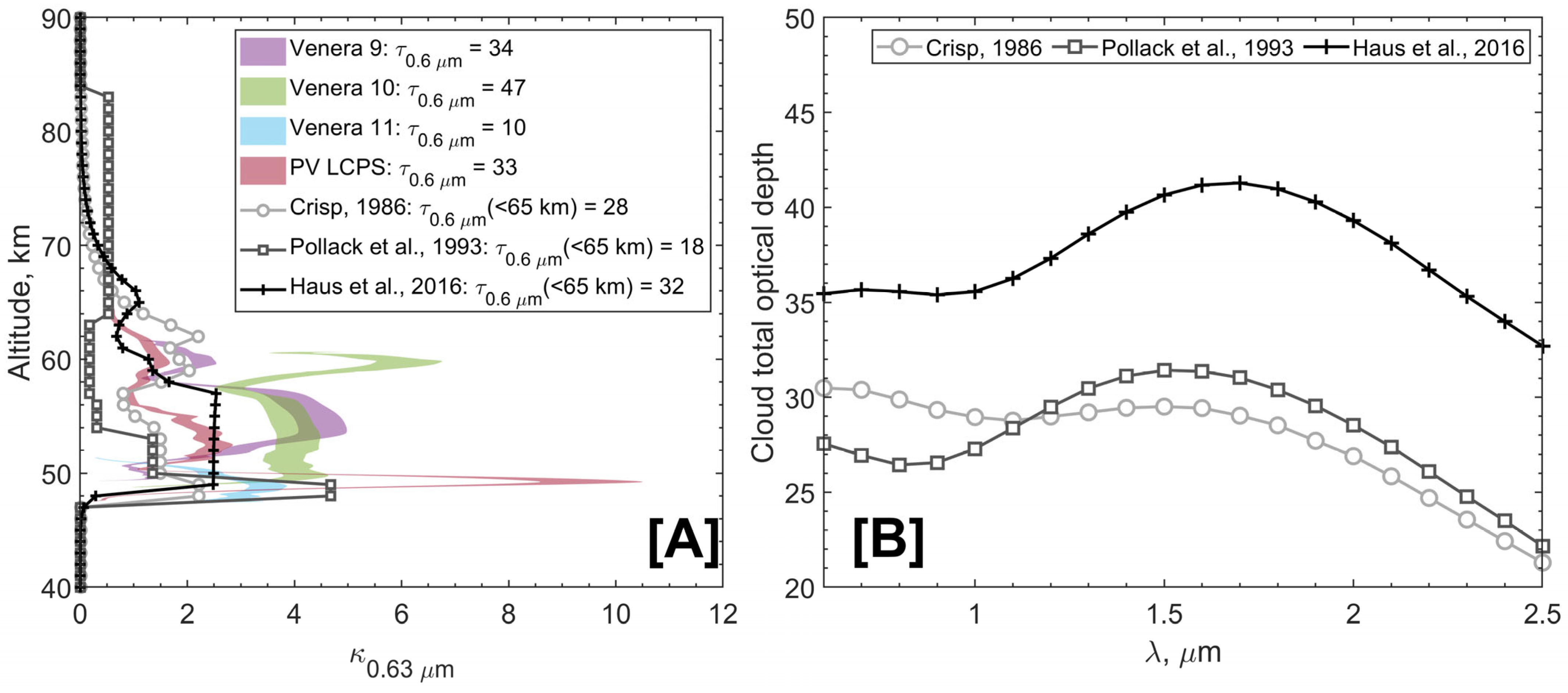
3.1. Cloud Layer Model

Generalized models based on observations are used to describe the scattering and absorption by aerosol particles in the transparency windows. It is assumed that aerosol particles are spherical and consist of an aqueous solution of sulfuric acid. The refractive index of H₂SO₄ solutions of different concentrations at 300 K was taken from [52]. The temperature in the lower and middle cloud layers varies from 370 K to 230 K according to the VIRA Climate Database [53]. Absorption by the H₂SO₄ aerosol of any concentration is negligible at wavelengths of 1–1.5 µm [52].

For our work, we use a cloud model from [46], thereafter the cloud model, where the cloud layer structure is described by simple analytical expressions for the vertical distribution of the numerical particle concentration of the four modes. This representation was derived from the observations by the VIRTIS-M/Venus Express spectrometer [33,46]. It assumes the lower and middle cloud layers to be homogeneous. In the cloud model, the upper cloud boundary on Venus, τ = 1 at 1 μm, is at 71 km. Previously, other cloud representation was used [39,54] where the vertical distribution of optical depth was set at 0.63 μm. Total cloud opacity has a weak spectral dependence in the range 0.6–1 μm for all the models (Figure 2). The cloud optical depth, evaluated at 0.6 μm and 1 μm, differs by less than 0.3% for the models of Refs. [39,46] and by 5% for the model of Ref. [54]. Thus, cloud opacity at 0.6 μm and 1 μm can be directly compared.

The three-layer cloud model from Ref. [46] is represented by particles of four modes: 1, 2, 2′ and 3. Each of the modes follows a log-normal size distribution. The effective radius and the dimensionless dispersion of modes 1, 2, 2′ and 3 are 0.3, 1.0, 1.4, and 3.65 μm and 1.56, 1.29, 1.23, 1.28, respectively [39,46]. Aerosol particle distributions in the clouds are set by vertical profiles of the number densities according to Equation (1) and

Table 1. Parameters in Equation (1) of the standard cloud model by Ref. [46].

Aerosol Particle Mode	1	2	2′	3
Lower base of peak altitude zb, km	49.0	65.0	49.0	49.0
Layer thickness of constant peak particle number zc, km	16.0	1.0	11.0	8.0
Upper scale height Hup, km	3.5	3.5	1.0	1.0
Lower scale height Hlo, km	1.0	3.0	0.1	0.5
Particle number density N0 at zb, cm−3	193.5	100	50	14

.

$$N\left(z\right)=\left\{\begin{array}{c}{N}_0\left(z_b\right)\exp \left(-{\displaystyle \frac{z-\left(z_b+z_c\right)}{H_{up}}}\right), z>(z_b+z_c)\\ N_0\left(z_b\right), (z_b+z_c)\ge z\ge z_b\\ N_0\left(z_b\right)\exp \left(-{\displaystyle \frac{z_b-z}{H_{lo}}}\right), z<z_b\end{array}\right\}$$

(1)

The real part of the refractive index and its dependence on the wavelength are close for different concentrations of sulfuric acid solution in the spectral range 1.25–1.32 μm. The resulting difference in the optical depth of the cloud layer when using the concentration values of 75% and 95.6% is less than 1%. In our study, the concentration in the cloud model is fixed to 75%. The aerosol extinction, single-scattering albedo and the Legendre expansion coefficients of phase functions are computed using the Mie theory [55] for each mode.

3.2. Numerical Model for Solving the Radiative Transfer Equation

Transparency window spectra are calculated using a one-dimensional multiple scattering radiative transfer model built with the DISORT4 program package [56,57]. It implements the discrete ordinate method in a plane-parallel or pseudo-spherical geometry. Radiative transfer is solved for 16 streams. Emission angles of 60–78° constitute 1% of the analyzed dataset where the pseudo-spherical approximation is necessary. DISORT4 has been found to consume less computational time than the SHDOMPP package, which implements the spherical harmonics and discrete ordinate method for radiative transfer in a plane-parallel atmosphere [58]. The latter is an iterative method, and the number of iterations increases in optically thick media since the single scattering albedo value approaches 1.

A wavelength grid is set with a step of 0.1 cm⁻¹. A decrease in this parameter has no impact on the result due to the SPICAV spectral resolution [50]. Convolution with the instrument function is performed on the model spectrum. The instrument function, i.e., the AOTF spectral response function, has been updated in this study (for more details, see Supplementary Material, Figure S1). The wavelength calibration of the spectra was obtained with an accuracy better than 0.2 nm on average [59]. This minor correction is adjusted for each spectrum individually by considering a wavelength shift as a free parameter of the spectrum optimization problem.

A uniform initial division of the atmosphere into discrete homogeneous layers of 1 km from the surface up to 100 km is performed. The structure of the atmosphere is represented by vertical profiles of temperature and optical parameters of the medium: the optical depth of computational layers, single scattering albedo and the Legendre series expansion of the particle scattering phase function. Vertical profiles of temperature, pressure, and density were taken from the Venus International Reference Atmosphere (VIRA) [53] and the Venus Climate Database (VCD) [60]. VIRA from 0 to 100 km is derived from a synthesis of data from the Pioneer Venus landers and orbiter, and the Venera-10, 12 and 13 landers [53]. The VCD is based on current Venus global climate model results [60]. At altitudes below 15 km, VIRA temperature profiles differ from the VCD values. On average, they are 2 K higher than those in the VCD. We used both databases and studied the sensitivity of the results.

The absorption of carbon dioxide and water vapor is included in the model. The CO₂ mixing ratio is set to 0.965. The CO₂ absorption is computed using a high-temperature spectral database AMES [61,62,63]. It is known that absorption in the wings of the CO₂ lines is smaller than that described by the Lorentz line shape. In our work, absorption in the line wings is corrected by the χ-factor [64]. The profile extends from the center of each line up to 250 cm⁻¹. The carbon dioxide continuum absorption at high temperatures and pressures, which is proportional to the squared density, was taken into account [59,64]. The continuum is a superposition of far wings of strong CO₂ bands, collision-induced transitions, and absorption by molecule dimers. In the model, this part of the absorption is represented by the binary coefficient α. Its possible values were constrained for the 1.1 and 1.18 µm transparency windows in the ranges (0.29–0.66) × 10⁻⁹ cm⁻¹amagat⁻² and (0.30–0.78) × 10⁻⁹ cm⁻¹amagat⁻², respectively, for the “High-T” spectral database [59]. The CO₂ Rayleigh scattering cross-section is calculated following [9,10,65]. We recomputed the obtained continuum coefficient using the AMES line list and the line shape parameters presented in

Table 2. A summary of the parameters and methods used in the radiative transfer model of 1.28 and 1.31 μm transparency windows.

Radiative transfer solver	DISORT4 [56,57] in pseudo-spherical geometry with 16 streams Line-by-line computation on wavelength grid with a step of 0.1 cm−1
Atmosphere structure	(1) Venus International Reference Atmosphere (VIRA) [53] (2) Venus Climate Database (VCD) [60]
Cloud model	Aerosol number density set by Equation (1) and Table 1 [46] Effective radius of aerosol modes 1, 2, 2′ and 3: 0.3, 1.0, 1.4, and 3.65 μm [39,46] Dispersion of aerosol modes 1, 2, 2′ and 3: 1.56, 1.29, 1.23, and 1.28 [39,46] Aerosol composition: water solution of H2SO4 with concentration of 75% Aerosol particle shape: spherical H2SO4 refractive index [52] Optical depth, single scattering albedo and Legendre series expansion of particle scattering phase function are calculated using Mie theory
CO2 absorption and molecular scattering	Line list: AMES [61,62,63] Line shape: sub-Lorentzian profile [64] Line cut-off: 250 cm−1 CO2 continuum: <2 × 10−9 cm−1amagat−2 CO2 volume mixing ratio: 0.965 Rayleigh scattering [9,10,65]
H2O absorption	Line list: BT2 [66] Line shape: Voigt profile Line cut-off: 180 cm−1 H2O volume mixing ratio: 28 × 10−6 (28 ppm)
Surface emissivity	0.95
Surface topography	Magellan data [51]
O2 (a1Δg) airglow	Line-by-line model [67,68]
Model free parameters	(1) Scaling factor applied on particle number density vertical profiles of modes 2, 2′ and 3 (2) Column density of O2* molecules (3) Scalar wavelength shift

. When analyzing the data of the 1.28 and 1.31 μm transparency windows, we considered the continuum absorption in the (0.4–1.0) × 10⁻⁹ cm⁻¹amagat⁻² range.

H₂O is assumed to be uniformly distributed under clouds with a volume mixing ratio of 28 ppm (parts per million) [47,59]. The sensitivity to changes in water vapor content is negligible for the transparency window at 1.28 μm (Figure 3C). The 1.31 μm transparency window has minor sensitivity to possible H₂O variations (Figure 3C). The deviation of 5% predicted by the model is lower in absolute values (~0.7 mW/m²/μm/sr) than the noise level (>1 mW/m²/μm/sr) in all cases. The H₂O absorption is computed using a high-temperature line list, BT2 [66]. The H₂O line shape is set by the Voigt profile, with the wings extended up to 180 cm⁻¹.

The surface temperature is adjusted to the atmospheric value at the local elevation calculated from Magellan data as the average within the instrument’s footprint [51]. The Venus surface emissivity is set to 0.95. The radiation is less than 1% sensitive to changes in emissivity (Figure 3B). The emission angles of points, corresponding to the center and at the perimeter of the SPICAV IR footprint, are defined by the angular size of the instrument’s field of view and the distance from the spacecraft to Venus’ surface. For distant observations, it is important to consider the distribution of emission angles, which is determined by the observation geometry. The synthetic emission is then averaged over the interval of emission angles obtained.

Emission in the 1.28 and 1.31 μm transparency windows is mainly determined by atmospheric conditions at 0–15 km (Figure 3A). The measured radiance is modulated by variations in the cloud optical depth, since there are no strong absorption bands of minor atmospheric constituents in this range. For our work, the three-layer cloud model [46] is considered and is discussed in Section 3.1. Figure 3D–G show that it is not possible to correlate the variation of the transparency window radiance with the height of the variation of the aerosol particle content. The radiance is sensitive to the whole cloud layer, i.e., the total amount of aerosol particles. Sensitivity to the aerosol abundance variation does depend on particle size. The radiance change due to the insertion of mode 3 particles exceeds that of mode 2′, 2 and 1 by a factor of 4.5, 8.5 and 128, respectively. For the 1.31 µm transparency window, the values obtained are 4.6, 8.8 and 135. Thus, we can neglect the influence of mode 1 but not the contribution of mode 2 and 2′ particles. This is performed in the model by the multiplication of the vertical profiles of the mode 2, 2′ and 3 number densities N (Equation (1)) by a scaling factor. For the three modes, the scaling factor is the same. The ratio of differently sized particles in the cloud and even the concentration of H₂SO₄ in aerosol droplets can be deduced by analyzing the spectrum in a wider range than the narrow interval of 1.28 and 1.31 µm transparency windows.

The latitudinal dependence of the upper cloud boundary is known from the data from several experiments [27,28,29]. In the equatorial region, the upper boundary is located at 72 km, while at the polar latitudes, it drops to 61–67 km. In our work, the upper bound of the vertical distribution of aerosol particles of modes 1 and 2 at latitudes greater than 40° is corrected accordingly by constraining the thickness of these mode layers in the cloud model.

There is a band of O₂ (a¹Δ_g) airglow around 1.27 μm that overlaps the spectral range of the 1.28 μm transparency window (Figure 4). The airglow forms at an altitude of 96 km [39]. We follow the algorithm applied to the terrestrial ¹⁶O₂ (a¹Δ_g) airglow spectrum [67,68]. The airglow spectrum is calculated with an assumption of a constant rotational temperature of 195 K. The value is the mean rotational temperature of O₂* from ground-based observations [69]. At an altitude of ~95 km, pressure and temperature are low, but the individual O₂ airglow lines are not resolved due to the wide SPICAV instrument function. Self-absorption of O₂ and absorption of CO₂ in the upper atmosphere can be neglected, and the airglow spectrum per molecule is multiplied by the column number density of O₂* molecules. The resulting airglow spectrum is added to the thermal radiation of Venus.

Parameters that provided the minimum reduced χ²-value of the experimental and modeled spectra were considered as the solution. The computation of reduced χ² considers the 1.235–1.315 μm spectral range. Overall, each spectrum is fitted by tuning three parameters in the model using the simplex algorithm [70]:

• The scaling factor of the vertical profiles of the mode 2, 2′ and 3 particle number densities;
• The column number density of O₂* molecules;
• The scalar wavelength shift of the wavelength calibration.

The resulting cloud optical depth can be evaluated using the aerosol extinctions [55] and number density profiles of four modes, where the obtained scaling factor is applied to densities of modes 2, 2′ and 3. A summary of all the model parameters is presented in Table 2. Examples of the spectrum fitted by the model are presented in Figure 4. Figure 4 cover different cases including high (Figure 4D,F) or low (Figure 4B) cloud optical depths, different topography of the observed areas (Figure 4A–C) and the presence of bright O₂ (a¹Δ_g) airglow (Figure 4E,F).

4. Result

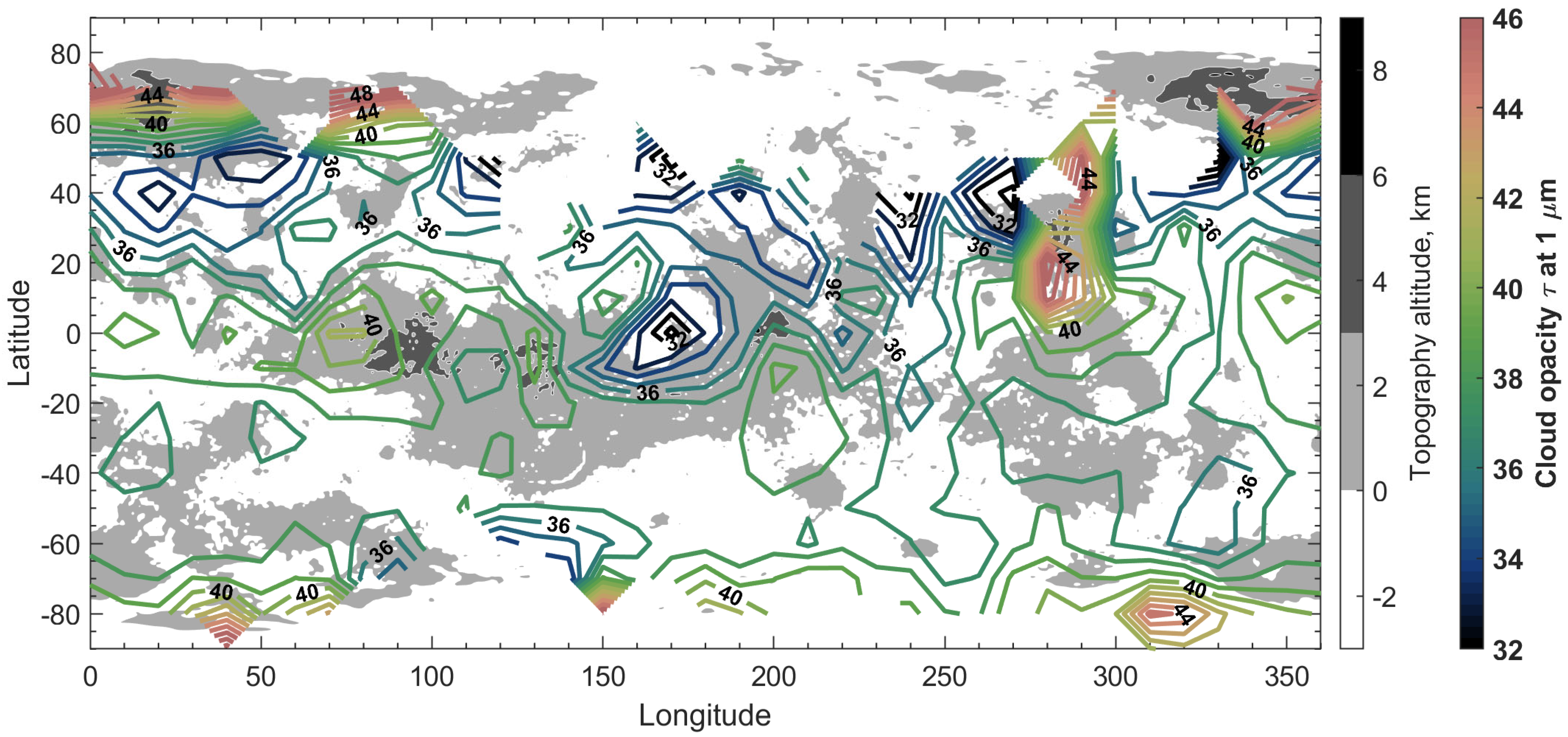
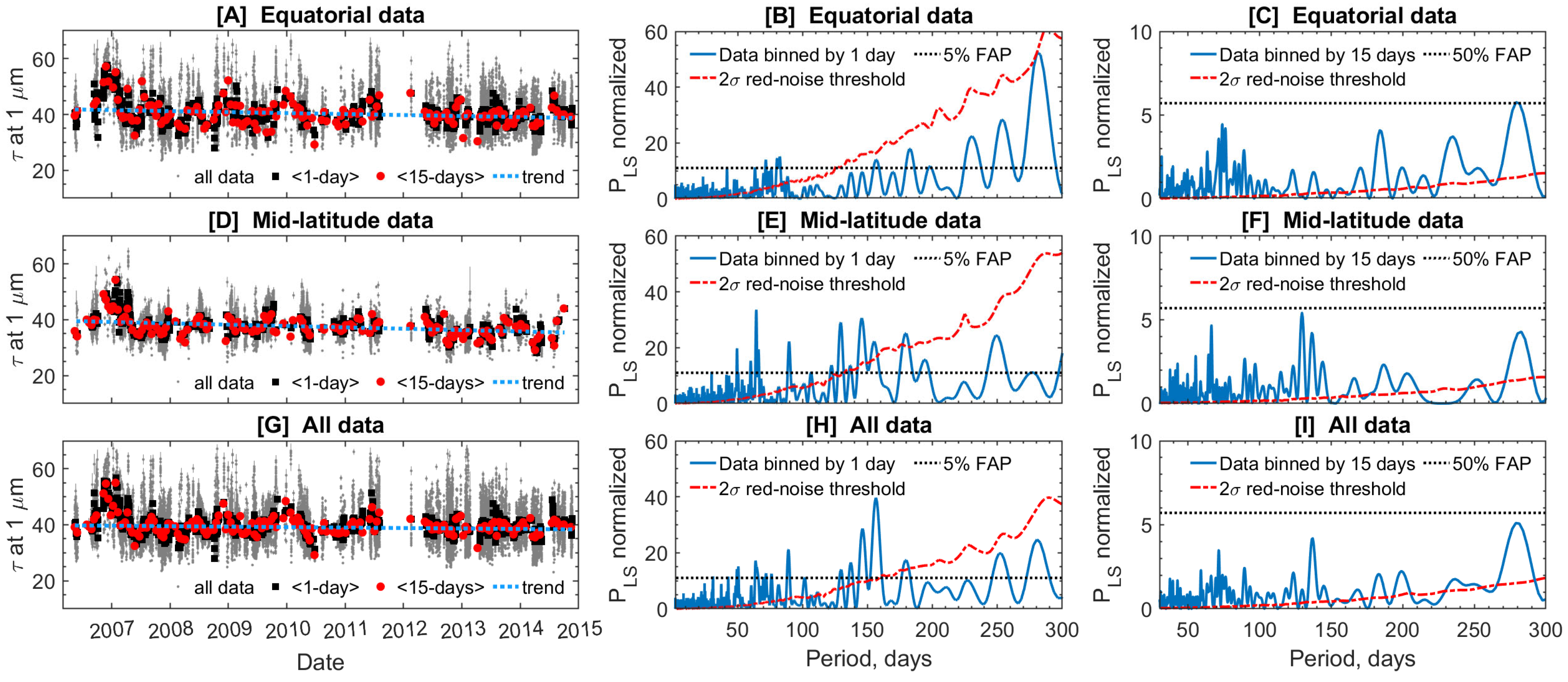
4.1. Venus Cloud Optical Depth Spatial Distribution and Temporal Behavior

Data processing results in the values of the scaling factor of the particle number density common for the 2, 2′ and 3 modes. As described in Section 3.1, the scaling factor is converted to the cloud layer optical depth by multiplying the extinction and number density profile of each aerosol mode. Optical depth is spectrally dependent. We compute the optical depth at a wavelength of 1 μm. At shorter wavelengths, the spectral dependence of the optical depth is weak (Figure 2B). The weighted average of the scaling factor for all observations, using the measurement error as weight, is 1.03. The standard deviation is equal to 0.19. The corresponding optical depth at 1 μm is 36.7 ± 6.1. The values are obtained using the CO₂ continuum coefficient α = 0.6 × 10⁻⁹ cm⁻¹amagat⁻² and the VIRA temperature profile [53].

Significant variability is observed, and errors of the measured values are smaller than the variations. The relative error of the optical depth extracted from a spectrum is between 1 and 9%, and the average error is 2%. Optical depth is observed between 23 and 67 (Figure 5). However, 4% of the values are optical depths less than 25 and greater than 50. There are nine observations with a recorded minimum optical depth spread over the entire longitude range and 2–53° N latitude. Clouds with high optical depth were observed much more frequently than those with τ < 25. Clouds with optical depths above 50 were detected mainly above 60° N and 50° S and between 30° S and 30° N. At high latitudes, values above 60 are characteristic of the Ishtar Land region, above 60° N. This is explained by the observational selection (Figure 2). In the equatorial region, the distribution of the optical depths above 50 are sporadic and no correlation was found between cloud opacity and topographical features.

The zonal mean of the total optical depth at 1 μm shows latitudinal dependence (Figure 5). A symmetrical distribution with respect to the equator can be expected as an increase in optical depth is observed above 50° S. However, tens of degrees of latitude can be covered by the SPICAV IR field of view in the Southern Hemisphere. The averaging takes into account the footprint. In the Southern Hemisphere it is impossible to study the latitudinal distribution of clouds with high-latitude resolution. The decrease in mean optical depth from 80° S to the South Pole is also an effect of averaging over large areas. In the Northern Hemisphere, the size of the footprint decreases. For latitudes above 30° N, the footprint is smaller than the bin side. The mean value of optical depth is approximately constant up to 20° N, and then decreases to a minimum value of 32.7 ± 5.4 at 50–55° N. At polar latitudes, cloud opacity increases rather monotonically and significantly, despite the decreasing observational statistics.

The number density scaling factors that provide the observed variations in optical depth correspond to the upper boundary of clouds, i.e., τ = 1, equal to 69–73 km at the equator and ~64 km at 80° N. The latter is about 2 km higher than that obtained from VIRTIS-M data [46]. In the work of [46], a wider spectral range was considered, and the particle content of the lower and middle cloud layers was varied separately, i.e., particles of modes 2′ and 3 and particles of modes 1 and 2 [46]. According to the VIRTIS-M data, the mode 2′ and 3 particle number density follows the optical depth trend and increases towards the polar regions, while the mode 1 and 2 aerosol particles diminish. In our approach, aerosol particles of modes 2, 2′ and 3 follow the same trend, which plausibly leads to an overestimation of the particle number density in the upper cloud layer and hence to an increase of the upper boundary (τ = 1). Such a conclusion can only be drawn based on further experiments, since the intensity of the 1.28 and 1.31 μm transparency windows depends almost equally on the mode 2′ and 2 densities.

The observation statistics accumulated over 8 years allow us to compile the geographical distribution of cloud optical depth. When the data are binned by 10° of latitude and 10° of longitude, 66% of the Venusian globe is covered (Figure 6). Looking at the geographical distribution obtained, it can be seen that the belt of minimum cloud depth is approximately constant in the 30–50° N region. A slight increase in the mean optical depth is noticed in the areas of the main surface elevations of Venus near the equator. However, no persistent correlation with the relief could be established due to the high variability of the values (Supplementary Material, Figure S2). Dependence on the local time of day could not be established either (Supplementary Material, Figure S3).

The SPICAV IR data, accumulated over 8 years of observations, allow us to assess the long-term variability of the cloud layer. A disadvantage of the dataset is the sparse spatial coverage at one orbit, i.e., one Earth day. The part of the night hemisphere that is observed during one orbit is 0.04–15%. Consequently, the observed areas usually do not overlap between several consecutive observational sessions. Observations of the Southern Hemisphere have the largest footprints, where the signal is exposed over the entire field of view. This makes it challenging to study temporal variation and separate it from the spatial features that are observed. The data show strong fluctuations on the short-term scale. The linear trend obtained for 8 years of observations shows a minor decrease (Δτ < 1) in the optical depth, and it is several times lower than the opacity fluctuations.

To analyze the long-term variability of cloud opacity, we grouped the observations in three sets: all observations and the equatorial (30° S–30° N) and mid-latitude (30–60° S and 30–60° N) regions. Within each group, the data are smoothed by moving averages with a window of 7 days to suppress the atmospheric superrotation period of ~7 Earth days at the lower cloud altitudes [22,23]. Then, the values are binned by 1 or 15 days and averaged within one bin. Binning by 15 days allows us to increase spatial coverage. The Lomb–Scargle periodogram is computed for the obtained optical depth values (Figure 7) eliminating the obtained weak linear trend in order to search for possible periodic phenomena. This method allows us to analyze unevenly sampled data as the SPICAV IR dataset. The sampling introduces additional noise to the Lomb–Scargle periodogram. To evaluate the statistical significance of the identified periodogram peaks, the false-alarm probability (FAP) threshold was determined. Moreover, atmospheric data are often autocorrelated time series [71,72], characterized by red noise whose spectral density increases with decreasing frequency [73]. In our work, the confidence level of the Lomb–Scargle periodogram in the low-frequency range is calculated by constructing 1000 random time series of red noise [71,74].

The periodograms for the 1-day binned dataset have maxima that dominate the 5% FAP threshold. There are weak peaks corresponding to periods of 70 and 80 Earth days for the equatorial region (Figure 7B). In the mid-latitudes, periods of about 60, 90, 130, 150 and 180 days can be selected according to the criteria applied (Figure 7E). Considering the whole dataset, time variations with a period of about 150 Earth days are highlighted (Figure 7H). Periods longer than 200 days are below the obtained red noise level. Data binning by 15 days does not reveal any of the harmonics mentioned and the periodogram peaks are below the 50% FAP threshold (Figure 7C,F,I). We therefore conclude that the SPICAV IR dataset does not provide sufficient evidence of long-term periodic fluctuations in cloud opacity due to uneven temporal and spatial sampling.

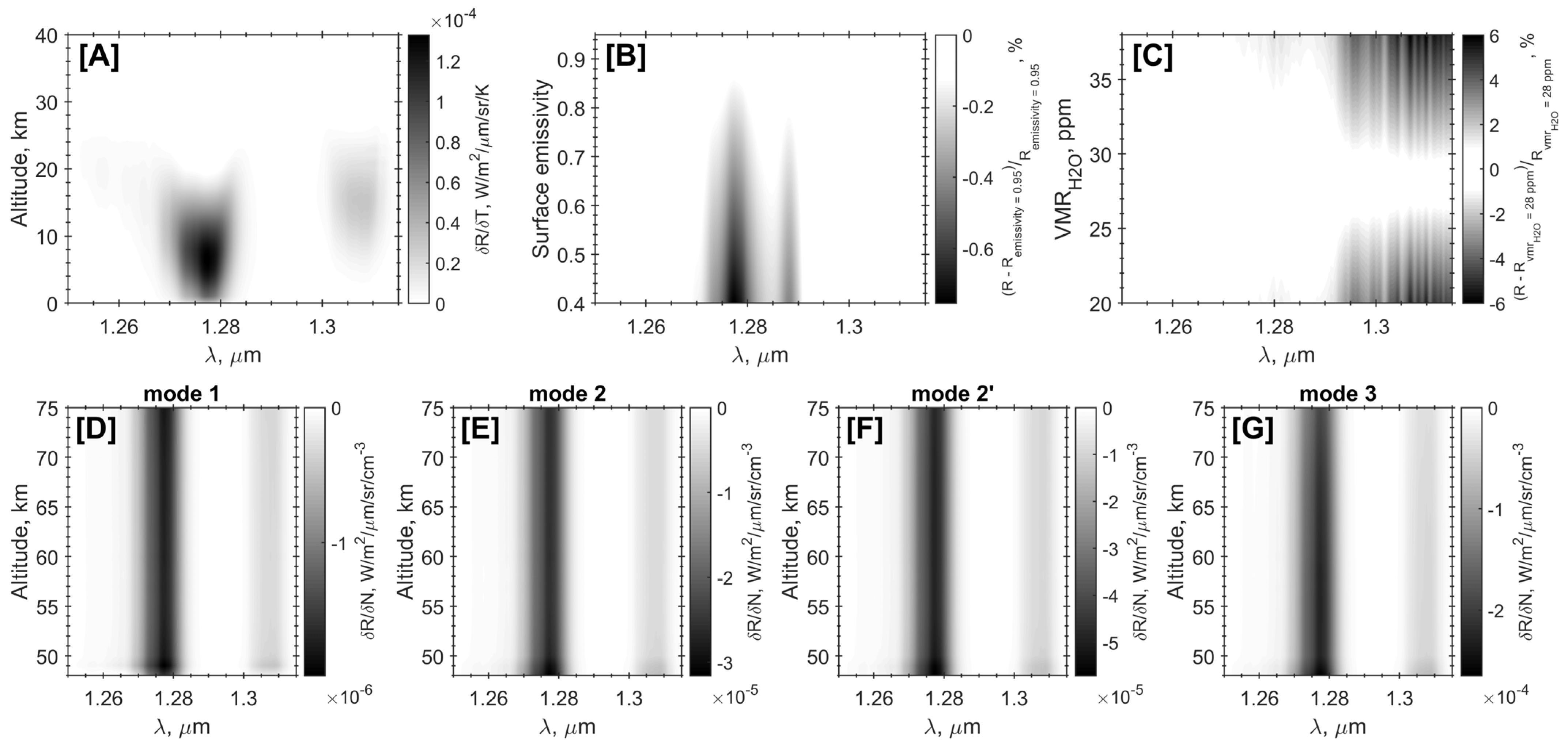
4.2. Investigation of Result Uncertainty

Atmospheric emission, absorption and scattering, which form the spectrum of the 1.28 and 1.31 µm transparency windows of Venus, are determined by a significant number of parameters. Conditions in Venus’ lower atmosphere have only been directly studied in a few regions where spacecraft have descended [36]. The large thermal inertia of the dense atmosphere should prevent diurnal variations in the deep atmosphere. The models of the Venus atmosphere considered above provide slightly different temperature and pressure profiles. On average, the VIRA temperature [53] in the near-surface layer is 2 K higher than the VCD values [60]. The measured surface and lower atmosphere temperatures are also within several degrees’ difference [36]. Figure 8 shows an example of spectrum analysis performed for different temperature and pressure profiles. Figure 8C shows that the VCD temperatures exceed the VIRA values below 20 km, and they are lower than the VIRA values at 20–40 km. This minor difference does not interfere the spectral shape of the windows, but it corrects the obtained cloud optical depth.

The results obtained with the fixed continuum factor α = 0.6 × 10⁻⁹ cm⁻¹amagat⁻² for the VIRA and VCD temperature profiles were compared. On average, the VIRA temperature in the near-surface layer is 2 K higher than the VCD values. The vertical temperature profile of the VCD, as well as density and pressure, has been set as the average over the SPICAV IR footprint. The resulting optical depth is, on average, Δτ = 2 less for VCD temperatures, but individual values can vary. It should be noted that the use of the alternative VIRA temperature profile does not change the obtained optical depth dependencies.

The spectroscopic parameters of the absorption lines at high temperatures and pressures are also subject to uncertainties. First, the various spectroscopic databases adapted to high temperatures are semi-empirical and have differences. In this study, the AMES line list [61,62,63] was preferred over the “High-T” database [39,59,64], which is commonly used [33,46,59,64] for the analysis of Venus transparency windows. The wavelength calibration shift is strongly dependent on the presence of a bright O₂ (a¹Δ_g) airglow feature in the spectrum (Figure 4) when CO₂ absorption is calculated using the “High-T” database. For cases where the O₂ (a¹Δ_g) airglow is brighter than 1 MR, the obtained wavelength shift is around zero. This is in agreement with the results obtained during the preparation of the instrument [50]. All observations of the O₂ (a¹Δ_g) airglow brighter than 1 MR lead to a nearly normal distribution of the obtained values with average of −0.028 and standard deviation of 0.091 (Figure 9B). However, if the airglow is weak or absent, the spectral shape of the window can only be recovered by a larger shift in the wavelength calibration. For the entire dataset, the obtained shift distribution shows several maxima (Figure 9A). The implementation of the AMES line list [61,62,63] improves the wavelength shift result. On average, it is equal to −0.086 ± 0.138 for the entire dataset and 0.004 ± 0.086 for the O₂ (a¹Δ_g) airglow intensity > 1MR.

Secondly, the CO₂ continuum parametrization is not defined with sufficient precision. The influence of continuum absorption, which is proportional to the squared density, decreases significantly with increasing surface elevation. Figure 10 shows the variation of the intensity at the maximum of the 1.28 and 1.31 μm transparency windows for cases with weak molecular oxygen airglow (<0.3 MR). The values are shown with the standard deviation of the intensity at the window maxima. The number of observations where surface elevation is greater than 2 km is much poorer, but the dependence on topography is traceable. Similar dependence is observed after removing the oxygen airglow. Figure 10 shows the modeled dependence of 1.28 and 1.31 μm radiance on surface elevation for the best-fitted cloud optical depth. According to the results of the data processing at α = 0.6 × 10⁻⁹ cm⁻¹amagat⁻², the weighted mean result is 36.7 and the average is 39.1. Coefficient α = 1.0 × 10⁻⁹ cm⁻¹amagat⁻² leads to a weighted mean of 31.8 and an average of 34.9, and α = 0.2 × 10⁻⁹ cm⁻¹amagat⁻² to 41.7 and 44.5, respectively. Thus, values of α = 0.2 × 10⁻⁹ cm⁻¹amagat⁻² and α = 1.0 × 10⁻⁹ cm⁻¹amagat⁻² correct the derived weighted mean of τ by 5.0 and −4.9, respectively. This correction is also systematic and does not alter the obtained temporal and spatial dependencies. The value of α = 0.2 × 10⁻⁹ cm⁻¹amagat⁻² is underestimated and only 83% of the optical depth values correspond to the 25–50 range, which is less consistent with previous observations. For α = 0.6 × 10⁻⁹ cm⁻¹amagat⁻², 96% of the values are obtained in the 25–50 range. For α = 1.0 × 10⁻⁹ cm⁻¹amagat⁻², 98% of the values correspond to the 25–50 range. Figure 10C presents the distributions of the retrieved values. The plotted dependencies for α = 0.6 × 10⁻⁹ cm⁻¹amagat⁻² and α = 1.0 × 10⁻⁹ cm⁻¹amagat⁻² demonstrate that it is challenging to determine which value of α is preferable. However, the obtained weighted mean value of the cloud optical depth at α = 1.0 × 10⁻⁹ cm⁻¹amagat⁻² is 31.8 ± 6.1, and it decreases to 28.8 ± 4.5 around 50° N. The results are summarized in

Table 3. Retrieved cloud optical depth at 1 μm depending on the CO₂ continuum binary coefficient.

CO2 Continuum Coefficient, α	Weighted Mean with STD	Weighted Mean with STD at 50° N	Percentage of Retrieved τ in Range of 25–50
0.2 × 10−9 cm−1amagat−2	41.7 ± 6.5	39.0 ± 5.2	83%
0.6 × 10−9 cm−1amagat−2	36.7 ± 6.1	32.7 ± 5.4	96%
1 × 10−9 cm−1amagat−2	31.8 ± 6.1	28.8 ± 4.5	98%

. We refer to the weighted mean in our study as it accounts for measurement error, which is dependent on the spectrum noise level. The obtained opacity for α = 1.0 × 10⁻⁹ cm⁻¹amagat⁻² is also smaller than the results from the VIRTIS-M data study [46], and α = 0.6 × 10⁻⁹ cm⁻¹amagat⁻² is chosen in our model. However, the presented analysis demonstrates the importance of further laboratory investigations of the CO₂ continuum.

5. Discussion

We present the first complete analysis of the 1.28 and 1.31 μm atmospheric transparency windows’ observations, adapting the Venus cloud layer model of [46] to obtain the total cloud optical depth. The simultaneous variation of aerosol particle modes 2, 2′ and 3 is sufficient to describe the observed variability. The upper cloud boundary is not a free parameter in this approach. But observations of the Venus cloud top altitude were taken into account, and the thickness of the mode 1 and 2 layers in the cloud model [46] was constrained. It was found that this approach still leads to an overestimation of the observed upper cloud boundary at polar latitudes. In order to reproduce the results of other experiments, it is therefore necessary to change the proportion of particles in the lower and upper cloud layers in the model. Thus, the abundance of modes 2′ and 3 should be increased, while the number of mode 1 and 2 particles should be reduced or unchanged. This result indirectly supports the conclusions derived from a robust analysis of the 1–2.5 μm range [31,32,33,34,46].

The continuum absorption by the CO₂ molecule at high pressures and temperatures in the lower atmosphere of Venus presents the largest uncertainty for cloud optical depth evaluation. Varying the coefficient α = 0.6 × 10⁻⁹ cm⁻¹amagat⁻² by ±40% changes the result by −13% and +14%, respectively. The chosen coefficient is equal to 0.6 × 10⁻⁹ cm⁻¹amagat⁻². This value leads to the weighted means, accounting for the experimental error, which are in the best agreement with previous observations [33,46,47]. The result at α = 1.0 × 10⁻⁹ cm⁻¹amagat⁻² gives a weighted mean optical depth of 31.8 ± 6.1 for the entire dataset and 28.8 ± 4.5 at 50° N. The CO₂ continuum is set empirically and depends on the absorption parameterization in the far wings of the CO₂ lines. In our work, we use the sub-Lorentzian line profile [64]. For the transparency window of 1.18 μm, the laboratory determined absorption coefficient is α = 0.55 × 10⁻⁹ cm⁻¹amagat⁻² [75]. This value includes absorption in the wings of the CO₂ lines and must be corrected for comparison with the values set in our work. In our study, the absorption line is extended to 250 cm⁻¹ from the center, so the laboratory measurement of α is ~0.3 × 10⁻⁹ cm⁻¹amagat⁻². The same value for the CO₂ continuum coefficient was obtained by considering α(1.28 μm) = 1.0 × 10⁻⁹ cm⁻¹amagat⁻² and the “High-T” CO₂ line list [59]. Recomputed for the AMES database [61,62,63], the CO₂ continuum coefficient is α(1.28 μm) = 0.6 × 10⁻⁹ cm⁻¹amagat⁻². It should also be noted that the upper limit of α(1.28 μm) was given as 2.0 × 10⁻⁹ cm⁻¹amagat⁻² [59], but in our work, we showed that this value would be an overestimate.

The resulting weighted mean optical depth is 36.7 ± 6.1 for 1 μm. There is considerable variability in the individual values from 22 to 72, but 96% of the observations correspond to the range 25–50. Such values have been observed by measurements in transparency windows by the NIMS spectrometer [44], the ground-based facility [47] and the VIRTIS-M experiment [33,46]. A summary of the cloud opacity measurements is presented in

Table 4. Measurements of the total cloud opacity in the Venus transparency windows.

Total Cloud Opacity	Instrument and Reference
τ = 25–40	Descend probes [1]
τ = 25–50	NIMS/Galileo spacecraft [39,44]
τ = 32–42 with <τ> = 36.5 at 1 μm	VIRTIS-M/Venus Express [33,46]
τ = 17–22 of lower cloud layer that corresponds to total τ = 35–40	TripleSpec/Apache Point Observatory [47]
<τ> = 36.7 ± 6.1 at 1 μm for α = 0.6 × 10−9 cm−1amagat−2 <τ> = 31.8 ± 6.1 at 1 μm for α = 1.0 × 10−9 cm−1amagat−2	SPICAV IR/Venus Express [33,46]

. Aerosol particle density anomalies in clouds are also interesting because the chemical sources of sulfuric acid, water vapor and sulfur dioxide, have volcanic origin. The possibility of indirectly confirming the presence of volcanic activity on Venus by remote observations of atmospheric components is widely discussed. However, calculations show that it is difficult to directly link increases in cloud optical depth to events on the planet’s surface [76]. Our study shows episodic increases in the optical depth of the cloud layer strictly at the equatorial and polar latitudes, with no clear link to any particular region on the surface. The zonal mean of the cloud optical depth shows clear dependence on the northern latitude. In the range 40–55° N, its values reach a minimum (τ = 32.7 at 1 μm) and then increase. VIRTIS-M observations in the Southern Hemisphere of Venus show the same pattern [32,33,46]. The spread of the derived values is also much larger in the equatorial zone (40° S–40° N) than in the mid-latitude zone. Bright quasi-zonal bands have been observed in ground-based observations of the Venusian night side at 2.35 μm [38]. A recent series of observations in the 1–2.5 μm range also shows greater variability in cloud optical depth near the equator than at the mid-latitudes [47]. The formation of the observed increase in the aerosol abundance near the equator and near the poles is described by a two-dimensional model considering the meridional circulation [77]. At high latitudes, dense clouds accumulate as a result of the modeled meridional transport of aerosols in the upper atmosphere towards the poles. At low latitudes, the model leads to the convective lifting of concentrated H₂SO₄ vapors and their condensation in the middle cloud layer [77]. Latitudinal distributions of SO₂ and H₂O obtained over 2006–2014 by SPICAV at the day side of Venus were symmetrical and had maxima at lower latitudes. This also indicates the advection of these molecules from the deep atmosphere [29,78]. The volume mixing ratio of SO₂ at the cloud tops (~70 km) decreased towards the poles. Enhanced values of the SO₂ VMR at 51–54 km were observed in the equatorial region and at polar latitudes in the radio occultation experiment [79]. The latitudinal distribution of water vapor at 61–63 km showed a minimum between 30° and 50° of latitude in both hemispheres and then an increase towards the poles [29]. However, the poleward increase of the H₂O VMR was well correlated with the decrease of the sensing altitude from 61–63 km to 58–62 km. At the cloud tops, the H₂O VMR was distributed uniformly on average at 40° S–40° N with a steady increase towards the poles [80]. The zonal mean of the upper boundary of the cloud layer shows a symmetric latitudinal distribution with respect to the equator [32,33,46]. The Southern Hemisphere VIRTIS-M and Northern Hemisphere SPICAV IR observations show that the total optical depth is also characterized by symmetry with respect to the equator. This picture cannot be obtained from SPICAV IR data alone because the instrument’s low spatial resolution in the Southern Hemisphere smooths out the plausible dependence of optical depth on latitude.

It is well established that the spatial and temporal variability of the Venus atmosphere within and above the cloud layer is significant. Observations of wind speed at the cloud tops showed a periodicity of 117 Earth days related to the influence of the underlying topography [81]. In addition, a period of 255 Earth days was observed, which is longer than the Venusian day—243 days [82]. The longest wind speed periodicity, exhibiting a 12-year cycle, is obtained by the Venus Express and Akatsuki spacecraft cameras [83]. The ultraviolet albedo at 365 nm showed a factor of two decrease from the maximum that occurred in 2006–2007 to a minimum in 2011–2014. Recent observations in 2016–2017 indicated an albedo increase to the level of 2008–2009 [84]. Such a long-term evolution was suggested to be linked to the solar cycle. In contrast with the cloud top observations, the total cloud opacity obtained in this study over 8 years shows only a minor decrease with Δτ < 1. Sulfuric acid is synthesized and condensed in the upper cloud layer [2]. A periodicity of SO₂, one chemical source of H₂SO₄, with harmonics of 400, 155, 110 and 113 Earth days and short periods (40, 17 and 6 Earth days) was obtained from cloud top observations in UV [78]. The abundance of water vapor, the second precursor of H₂SO₄, was monitored at 59–66 km and showed a remarkable variability, although without explicit periodicity [29]. The harmonic with a period of ~150 Earth days was identified in the radiance of the 1.74 and 2.3 μm transparency windows from VIRTIS-M observations of the Southern Hemisphere in 2006–2009 [85]. The variations were associated with changes in the opacity of Venus clouds and were most pronounced at 30–60° S. The two-dimensional atmospheric circulation model [77] predicts an overturning period of the Hadley-type meridional circulation of 90 Earth days at the cloud tops. It was concluded that the 150-day period of the 1.74 and 2.3 μm window intensity is most likely maintained by the interaction between radiative cooling and cloud microphysical processes [85]. The temporal patterns of Venus clouds were investigated as a function of the properties of the condensation nuclei [86]. In the presence of condensation, a population of nuclei incapable of growth results in an optical depth decrease, which can lead to long-term changes (several hundred days) in all cloud layers [86].

The lack of the imaging capability of SPICAV IR complicates the search for global periodicity and requires averaging over large areas. The SPICAV IR temporal coverage was uneven over the course of the Venus Express science mission. To improve spatial and temporal coverage for periodicity analysis, data should be clustered over a wide range of latitudes and average in time intervals. Cloud optical depth, binned by 1 days and averaged within one bin, reveals a potential periodicity of approximately 150 days, consistent with the VIRTIS-M observations. This harmonic is not observed at equatorial latitudes. At mid-latitudes, the cloud optical depth periodicity of about 60, 90, 130 and 150 days may be suggested. In order to achieve a wider spatial coverage of the night hemisphere, periodicity analysis was also conducted on the data binned by 15 days. The resulting periodograms revealed no explicit harmonics. Thus, the SPICAV dataset does not provide strong evidence of long-term periodicity in the cloud optical depth over 8 years of observations.

6. Conclusions

Here, we presented the first complete analysis of Venus cloud layer variability. The study is conducted based on the 1.28 and 1.31 μm atmospheric transparency window observations by the SPICAV IR spectrometer on board the Venus Express spacecraft in 2006–2014. The nadir spectra of the Venus night side were fitted to a one-dimensional multiple scattering radiative transfer model that comprises the thermal emission and the O₂ (a¹Δ_g) airglow. The temperature profile in the deep Venusian atmosphere and the CO₂ continuum due to the collision-induced absorption and extreme far wings of strong CO₂ bands are defined with uncertainty and cannot be solely derived from the existing dataset. The influence of these uncertainties on the resulting cloud opacity was studied in detail to quantify their reasonable constraints. The mean cloud opacity differed by Δτ = 2 between the VIRA and VCD temperature profiles. The assumption of the CO₂ continuum parametrization in the 1.28 and 1.31 μm transparency windows remained the greatest difficulty in the total cloud optical depth analysis, and this demonstrated the importance of its further laboratory investigation. The binary continuum coefficient of 0.6 × 10⁻⁹ cm⁻¹amagat⁻² provided the best agreement with previous observations [33,46,47] of cloud optical depth and was consistent with the laboratory determined absorption coefficient at 1.18 μm [75]. The CO₂ continuum of 1.0 × 10⁻⁹ cm⁻¹amagat⁻² reduces the cloud opacity by Δτ = 4.9 (Table 3 and Table 4).

The weighted mean of the optical depth at 1 μm is 36.7 with a standard deviation of 6.1 (Table 4). The latitudinal distribution exhibits a minimum of the cloud optical depth at 50–55° N, corresponding to a value of 32.7 ± 5.4 (Figure 5). A similar latitude dependence of the opacity was observed in the Southern Hemisphere by VIRTIS-M [33,46]. SPICAV IR spatial resolution in the Southern Hemisphere is poor due to the eccentricity of the spacecraft’s orbit and the latitudinal distribution of clouds is less pronounced. No prominent dependency on longitude was detected.

Our work shows that the Venus cloud layer is a very variable environment. The individual values vary between 23 and 67, and only 4% of the observations do not encompass the range of 25–50. The greatest variability of the cloud opacity was observed in the equatorial region, and the lowest variability at the mid-latitudes. However, long-term analysis revealed no prominent trend. Sparse spatial coverage at one orbit due to the lack of imaging capability makes it challenging to conclude the existence of periodic patterns in the clouds.

References

1. Esposito, L.W.; Knollenberg, R.G.; Marov, M.Y.A.; Toon, O.B.; Turco, R. The clouds and hazes of Venus. In Venus; Hunten, D.M., Colin, L., Donahue, T.M., Moroz, V.I., Eds.; The University of Arizona Press: Tucson, AZ, USA, 1983; pp. 484–564. [Google Scholar]
2. Titov, D.V.; Ignatiev, N.I.; McGouldrick, K.; Wilquet, V.; Wilson, C.F. Clouds and hazes of Venus. Space Sci. Rev. 2018, 214, 126. [Google Scholar] [CrossRef]
3. Sill, G.T. Sulfuric acid in the Venus clouds. CoLPL 1972, 9, 191–198. [Google Scholar]
4. Young, A.T. Are the Clouds of Venus Sulfuric Acid? Icarus 1973, 18, 564–582. [Google Scholar] [CrossRef]
5. Hansen, J.E.; Hovenier, J.W. Interpretation of the polarization of Venus. J. Atmos. Sci. 1974, 31, 1137–1160. [Google Scholar] [CrossRef]
6. Pollack, J.B.; Erickson, E.F.; Witteborn, F.C.; Chackerian, C.; Summers, A.L.; van Camp, W.; Baldwin, B.J.; Augason, G.C.; Caroff, L.J. Aircraft Observations of Venus’ Near-Infrared Reflection Spectrum: Implications for Cloud Composition. Icarus 1974, 23, 8–26. [Google Scholar] [CrossRef]
7. Dollfus, A.; Auriere, M.; Santer, R. Wavelength dependence of polarization. XXXVII. Regional observations of Venus. Astron. J. 1979, 84, 1419–1436. [Google Scholar] [CrossRef]
8. Sato, M.; Travis, L.D.; Kawabata, K. Photopolarimetry Analysis of the Venus Atmosphere in Polar Regions. Icarus 1996, 124, 569–585. [Google Scholar] [CrossRef]
9. Luginin, M.; Fedorova, A.; Belyaev, D.; Montmessin, F.; Wilquet, V.; Korablev, O.; Bertaux, J.-L.; Vandaele, A.C. Aerosol properties in the upper haze of Venus from SPICAV IR data. Icarus 2016, 277, 154–170. [Google Scholar] [CrossRef]
10. Luginin, M.; Fedorova, A.; Belyaev, D.; Montmessin, F.; Korablev, O.; Bertaux, J.-L. Scale heights and detached haze layers in the mesosphere of Venus from SPICAV IR data. Icarus 2018, 311, 87–104. [Google Scholar] [CrossRef]
11. Knollenberg, R.G.; Hunten, D.M. The microphysics of the clouds of Venus—Results of the Pioneer Venus particle size spectrometer experiment. J. Geophys. Res. 1980, 85, 8039–8058. [Google Scholar] [CrossRef]
12. Toon, O.B.; Ragent, B.; Colburn, D.; Blamont, J.; Cot, C. Large, solid particles in the clouds of Venus: Do they exist? Icarus 1984, 57, 143–160. [Google Scholar] [CrossRef]
13. Andreichikov, B.M.; Akhmetshin, I.K.; Korchuganov, B.N.; Mukhin, L.M.; Ogorodnikov, B.I.; Petryanov, I.V.; Skitovich, V.I. Chemical composition and structure of Venus clouds from results of X-ray radiometric experiments made with the Vega 1 and Vega 2 automatic interplanetary stations. Kosm. Issled. 1987, 25, 737–743. [Google Scholar]
14. Mills, F.P.; Allen, M. A review of selected issues concerning the chemistry in Venus’ middle atmosphere. Planet. Space Sci. 2007, 55, 1729–1740. [Google Scholar] [CrossRef]
15. Markiewicz, W.J.; Petrova, E.; Shalygina, O.; Almeida, M.; Titov, D.V.; Limaye, S.S.; Ignatiev, N.; Roatsch, T.; Matz, K.D. Glory on Venus cloud tops and the unknown UV absorber. Icarus 2014, 234, 200–203. [Google Scholar] [CrossRef]
16. Petrova, E.V. Glory on Venus and selection among the unknown UV absorbers. Icarus 2018, 306, 163–170. [Google Scholar] [CrossRef]
17. Tomasko, M.G.; Doose, L.R.; Smith, P.H. Absorption of Sunlight in the Atmosphere of Venus. Science 1979, 205, 80–82. [Google Scholar] [CrossRef]
18. Esposito, L.W. Ultraviolet contrasts and the absorbers near the Venus cloud tops. J. Geophys. Res. 1980, 85, 8151–8157. [Google Scholar] [CrossRef]
19. Ekonomov, A.P.; Moroz, V.I.; Moshkin, B.E.; Gnedykh, V.I.; Golovin Yu, M.; Crigoryev, A.V. Scattered UV solar radiation within the clouds of Venus. Nature 1984, 307, 345–347. [Google Scholar] [CrossRef]
20. Marov, M.I.; Lystsev, V.E.; Lebedev, V.N.; Lukashevich, N.L.; Shari, V.P. The structure and microphysical properties of the Venus clouds: Venera 9, 10, and 11 data. Icarus 1980, 44, 608–639. [Google Scholar] [CrossRef]
21. Zasova, L.V.; Moroz, V.I.; Linkin, V.M. Venera-15, 16 and VEGA mission results as sources for improvements of the Venus reference atmosphere. Adv. Space Res. 1996, 17, 171–180. [Google Scholar] [CrossRef]
22. Gierasch, P.J.; Goody, R.M.; Young, R.E.; Crisp, D.; Edwards, C.; Kahn, R.; McCleese, D.; Rider, D.; Del Genio, A.; Greeley, R.; et al. The general circulation of the Venus atmosphere: An assessment. In Venus II—Geology, Geophysics, Atmosphere, and Solar Wind Environment; Bucher, J.W., Hunten, D.M., Phillips, R.J., Eds.; University of Arizona Press: Tucson, AZ, USA, 1997; pp. 459–500. [Google Scholar]
23. Gorinov, D.A.; Zasova, L.V.; Khatuntsev, I.V.; Patsaeva, M.V.; Turin, A.V. Winds in the Lower Cloud Level on the Nightside of Venus from VIRTIS-M (Venus Express) 1.74 μm Images. Atmosphere 2021, 12, 186. [Google Scholar] [CrossRef]
24. Sánchez-Lavega, A.; Lebonnois, S.; Imamura, T.; Read, P.; Luz, D. The Atmospheric Dynamics of Venus. Space Sci. Rev. 2017, 212, 1541–1616. [Google Scholar] [CrossRef]
25. Svedhem, H.; Titov, D.V.; McCoy, D.; Lebreton, J.-P.; Barabash, S.; Bertaux, J.-L.; Drossart, P.; Formisano, V.; Häusler, B.; Korablev, O.; et al. Venus Express—The first European mission to Venus. Planet. Space Sci. 2007, 55, 1636–1652. [Google Scholar] [CrossRef]
26. Nakamura, M.; Imamura, T.; Ishii, N.; Abe, T.; Kawakatsu, Y.; Hirose, C.; Satoh, T.; Suzuki, M.; Ueno, M.; Yamazaki, A.; et al. AKATSUKI returns to Venus. Earth Planets Space 2016, 68, 75. [Google Scholar] [CrossRef]
27. Titov, D.V.; Taylor, F.W.; Svedhem, H.; Ignatiev, N.I.; Markiewicz, W.J.; Piccioni, G.; Drossart, P. Atmospheric structure and dynamics as the cause of ultraviolet markings in the clouds of Venus. Nature 2008, 456, 620–623. [Google Scholar] [CrossRef] [PubMed]
28. Ignatiev, N.I.; Titov, D.V.; Piccioni, G.; Drossart, P.; Markiewicz, W.J.; Cottini, V.; Roatsch, T.; Almeida, M.; Manoel, N. Altimetry of the Venus cloud tops from the Venus Express observations. J. Geophys. Res. Planets 2009, 114, E00B43. [Google Scholar] [CrossRef]
29. Fedorova, A.; Marcq, E.; Luginin, M.; Korablev, O.; Bertaux, J.-L.; Montmessin, F. Variations of water vapor and cloud top altitude in the Venus’ mesosphere from SPICAV/VEx observations. Icarus 2016, 275, 143–162. [Google Scholar] [CrossRef]
30. Zasova, L.V.; Ignatiev, N.; Khatuntsev, I.; Linkin, V. Structure of the Venus atmosphere. Planet. Space Sci. 2007, 55, 1712–1728. [Google Scholar] [CrossRef]
31. Lee, Y.J.; Titov, D.V.; Tellmann, S.; Piccialli, A.; Ignatiev, N.; Pätzold, M.; Häusler, B.; Piccioni, G.; Drossart, P. Vertical structure of the Venus cloud top from the VeRa and VIRTIS observations onboard Venus Express. Icarus 2012, 217, 599–609. [Google Scholar] [CrossRef]
32. Haus, R.; Kappel, D.; Arnold, G. Self-consistent retrieval of temperature profiles and cloud structure in the northern hemisphere of Venus using VIRTIS/VEX and PMV/VENERA-15 radiation measurements. Planet. Space Sci. 2013, 89, 77–101. [Google Scholar] [CrossRef]
33. Haus, R.; Kappel, D.; Arnold, G. Atmospheric thermal structure and cloud features in the southern hemisphere of Venus as retrieved from VIRTIS/VEX radiation measurements. Icarus 2014, 232, 232–248. [Google Scholar] [CrossRef]
34. Wilson, C.F.; Guerlet, S.; Irwin, P.G.J.; Tsang, C.C.C.; Taylor, F.W.; Carlson, R.W.; Drossart, P.; Piccioni, G. Evidence for anomalous cloud particles at the poles of Venus. J. Geophys. Res. Planets 2008, 113, E00B13. [Google Scholar] [CrossRef]
35. Tellmann, S.; Pätzold, M.; Häusler, B.; Bird, M.K.; Tyler, G.L. Structure of the Venus neutral atmosphere as observed by the Radio Science experiment VeRa on Venus Express. J. Geophys. Res. Planets 2009, 114, E00B36. [Google Scholar] [CrossRef]
36. Limaye, S.S.; Grassi, D.; Mahieux, A.; Migliorini, A.; Tellmann, S.; Titov, D. Venus Atmospheric Thermal Structure and Radiative Balance. Space Sci. Rev. 2018, 214, 102. [Google Scholar] [CrossRef]
37. Allen, D.A.; Crawford, J.W. Cloud structure on the dark side of Venus. Nature 1984, 307, 222–224. [Google Scholar] [CrossRef]
38. Crisp, D.; McMuldroch, S.; Stephens, S.K.; Sinton, W.M.; Ragent, B.; Hodapp, K.-W.; Probst, R.G.; Doyle, L.R.; Allen, D.A.; Elias, J. Ground-Based Near-Infrared Imaging Observations of Venus During the Galileo Encounter. Science 1991, 253, 1538–1541. [Google Scholar] [CrossRef]
39. Pollack, J.B.; Dalton, J.B.; Grinspoon, D.; Wattson, R.B.; Freedman, R.; Crisp, D.; Allen, D.A.; Bezard, B.; de Bergh, C.; Giver, L.P.; et al. Near-Infrared Light from Venus’ Nightside: A Spectroscopic Analysis. Icarus 1993, 103, 1–42. [Google Scholar] [CrossRef]
40. Meadows, V.S.; Crisp, D. Ground-based near-infrared observations of the Venus nightside: The thermal structure and water abundance near the surface. J. Geophys. Res. Planets 1996, 101, 4595–4622. [Google Scholar] [CrossRef]
41. Bézard, B.; De Bergh, C. Composition of the atmosphere of Venus below the clouds. J. Geophys. Res. Planets 2007, 112, E04S07. [Google Scholar] [CrossRef]
42. Taylor, F.W.; Crisp, D.; Bézard, B. Near-infrared sounding of the lower atmosphere of Venus. In Venus II—Geology, Geophysics, Atmosphere, and Solar Wind Environment; Bucher, J.W., Hunten, D.M., Phillips, R.J., Eds.; University of Arizona Press: Tucson, AZ, USA, 1997; pp. 325–351. [Google Scholar]
43. Crisp, D.; Sinton, W.M.; Hodapp, K.-W.; Ragent, B.; Gerbault, F.; Goebel, J.H.; Probst, R.G.; Allen, D.A.; Pierce, K.; Stapelfeldt, K.R. The Nature of the Near-Infrared Features on the Venus Night Side. Science 1989, 246, 506–509. [Google Scholar] [CrossRef]
44. Grinspoon, D.H.; Pollack, J.B.; Sitton, B.R.; Carlson, R.W.; Kamp, L.W.; Baines, K.H.; Encrenaz, T.; Taylor, F.W. Probing Venus’s cloud structure with Galileo NIMS. Planet. Space Sci. 1993, 41, 515–542. [Google Scholar] [CrossRef]
45. Drossart, P.; Piccioni, G.; Adriani, A.; Angrilli, F.; Arnold, G.; Baines, K.H.; Bellucci, G.; Benkhoff, J.; Bézard, B.; Bibring, J.-P.; et al. Scientific goals for the observation of Venus by VIRTIS on ESA/Venus express mission. Planet. Space Sci. 2007, 55, 1653–1672. [Google Scholar] [CrossRef]
46. Haus, R.; Kappel, D.; Tellmann, S.; Arnold, G.; Piccioni, G.; Drossart, P.; Häusler, B. Radiative energy balance of Venus based on improved models of the middle and lower atmosphere. Icarus 2016, 272, 178–205. [Google Scholar] [CrossRef]
47. Arney, G.; Meadows, V.; Crisp, D.; Schmidt, S.J.; Bailey, J.; Robinson, T. Spatially resolved measurements of H2O, HCl, CO, OCS, SO2, cloud opacity, and acid concentration in the Venus near-infrared spectral windows. J. Geophys. Res. Planets 2014, 119, 1860–1891. [Google Scholar] [CrossRef]
48. Barstow, J.K.; Tsang, C.C.C.; Wilson, C.F.; Irwin, P.G.J.; Taylor, F.W.; McGouldrick, K.; Drossart, P.; Piccioni, G.; Tellmann, S. Models of the global cloud structure on Venus derived from Venus Express observations. Icarus 2012, 217, 542–560. [Google Scholar] [CrossRef]
49. Bertaux, J.-L.; Nevejans, D.; Korablev, O.; Villard, E.; Quémerais, E.; Neefs, E.; Montmessin, F.; Leblanc, F.; Dubois, J.P.; Dimarellis, E.; et al. SPICAV on Venus Express: Three spectrometers to study the global structure and composition of the Venus atmosphere. Planet. Space Sci. 2007, 55, 1673–1700. [Google Scholar] [CrossRef]
50. Korablev, O.; Fedorova, A.; Bertaux, J.-L.; Stepanov, A.V.; Kiselev, A.; Kalinnikov, Y.K.; Titov, A.Y.; Montmessin, F.; Dubois, J.P.; Villard, E.; et al. SPICAV IR acousto-optic spectrometer experiment on Venus Express. Planet. Space Sci. 2012, 65, 38–57. [Google Scholar] [CrossRef]
51. Saunders, R.S.; Spear, A.J.; Allin, P.C.; Austin, R.S.; Berman, A.L.; Chandlee, R.C.; Clark, J.; deCharon, A.V.; De Jong, E.M.; Griffith, D.G.; et al. Magellan mission summary. J. Geophys. Res. 1992, 97, 13067–13090. [Google Scholar] [CrossRef]
52. Palmer, K.F.; Williams, D. Optical constants of sulfuric acid; application to the clouds of Venus? Appl. Opt. 1975, 14, 208–219. [Google Scholar] [CrossRef]
53. Seiff, A.; Schofield, J.T.; Kliore, A.J.; Taylor, F.W.; Limaye, S.S.; Revercomb, H.E.; Sromovsky, L.A.; Kerzhanovich, V.V.; Moroz, V.I.; Marov, M.Y. Models of the structure of the atmosphere of Venus from the surface to 100 kilometers altitude. Adv. Space Res. 1985, 5, 3–58. [Google Scholar] [CrossRef]
54. Crisp, D. Radiative forcing of the Venus mesosphere I. Solar fluxes and heating rates. Icarus 1986, 67, 484–514. [Google Scholar] [CrossRef]
55. Mishchenko, M.I.; Travis, L.D.; Lacis, A.A. Scattering, Absorption, and Emission of Light by Small Particles; Cambridge University Press: Cambridge, UK, 2002. [Google Scholar]
56. Lin, Z.; Stamnes, S.; Jin, Z.; Laszlo, I.; Tsay, S.-C.; Wiscombe, W.J.; Stamnes, K. Improved discrete ordinate solutions in the presence of an anisotropically reflecting lower boundary: Upgrades of the DISORT computational tool. J. Quant. Spectrosc. Radiat. Transf. 2015, 157, 119–134. [Google Scholar] [CrossRef]
57. Stamnes, K.; Tsay, S.-C.; Jayaweera, K.; Wiscombe, W. Numerically stable algorithm for discrete-ordinate-method radiative transfer in multiple scattering and emitting layered media. Appl. Opt. 1988, 27, 2502–2509. [Google Scholar] [CrossRef]
58. Evans, K.F. SHDOMPPDA: A Radiative Transfer Model for Cloudy Sky Data Assimilation. J. Atmos. Sci. 2007, 64, 3854–3864. [Google Scholar] [CrossRef]
59. Fedorova, A.; Bézard, B.; Bertaux, J.-L.; Korablev, O.; Wilson, C. The CO2 continuum absorption in the 1.10- and 1.18-μm windows on Venus from Maxwell Montes transits by SPICAV IR onboard Venus express. Planet. Space Sci. 2015, 113, 66–77. [Google Scholar] [CrossRef]
60. Martinez, A.; Lebonnois, S.; Millour, E.; Pierron, T.; Moisan, E.; Gilli, G.; Lefèvre, F. Exploring the variability of the venusian thermosphere with the IPSL Venus GCM. Icarus 2023, 389, 115272. [Google Scholar] [CrossRef]
61. Huang, X.; Schwenke, D.W.; Tashkun, S.A.; Lee, T.J. An isotopic-independent highly accurate potential energy surface for CO2 isotopologues and an initial 12C16O2 infrared line list. J. Chem. Phys. 2012, 136, 124311. [Google Scholar] [CrossRef]
62. Huang, X.; Freedman, R.S.; Tashkun, S.A.; Schwenke, D.W.; Lee, T.J. Semi-empirical 12C16O2 IR line lists for simulations up to 1500 K and 20,000 cm−1. J. Quant. Spectrosc. Radiat. Transf. 2013, 130, 134–146. [Google Scholar] [CrossRef]
63. Huang, X.; Gamache, R.R.; Freedman, R.S.; Schwenke, D.W.; Lee, T.J. Reliable infrared line lists for 13 CO2 isotopologues up to E′ = 18,000 cm−1 and 1500 K, with line shape parameters. J. Quant. Spectrosc. Radiat. Transf. 2014, 147, 134–144. [Google Scholar] [CrossRef]
64. Bézard, B.; Fedorova, A.; Bertaux, J.-L.; Rodin, A.; Korablev, O. The 1.10- and 1.18-μm nightside windows of Venus observed by SPICAV-IR aboard Venus Express. Icarus 2011, 216, 173–183. [Google Scholar] [CrossRef]
65. Sneep, M.; Ubachs, W. Direct measurement of the Rayleigh scattering cross section in various gases. J. Quant. Spectrosc. Radiat. Transf. 2005, 92, 293–310. [Google Scholar] [CrossRef]
66. Barber, R.J.; Tennyson, J.; Harris, G.J.; Tolchenov, R.N. A high-accuracy computed water line list. Mon. Not. R. Astron. Soc. 2006, 368, 1087–1094. [Google Scholar] [CrossRef]
67. Bertaux, J.-L.; Hauchecorne, A.; Lefèvre, F.; Bréon, F.-M.; Blanot, L.; Jouglet, D.; Lafrique, P.; Akaev, P. The use of the 1.27 µm O2 absorption band for greenhouse gas monitoring from space and application to MicroCarb. Atmos. Meas. Tech. 2020, 13, 3329–3374. [Google Scholar] [CrossRef]
68. Evdokimova, D.; Fedorova, A.; Zharikova, M.; Montmessin, F.; Korablev, O.; Soret, L.; Gorinov, D.; Belyaev, D.; Bertaux, J.-L. Night O2 (a1Δg) airglow spatial distribution and temporal behavior on Venus based on SPICAV IR/VEx nadir dataset. Icarus 2025, 429, 116417. [Google Scholar] [CrossRef]
69. Bailey, J.; Meadows, V.S.; Chamberlain, S.; Crisp, D. The temperature of the Venus mesosphere from O2 (a1Δg) airglow observations. Icarus 2008, 197, 247–259. [Google Scholar] [CrossRef]
70. Lagarias, J.C.; Reeds, J.A.; Wright, M.H.; Wright, P.E. Convergence Properties of the Nelder-Mead Simplex Method in Low Dimensions. SIAM J. Optim. 1998, 9, 112–147. [Google Scholar] [CrossRef]
71. Kopparla, P.; Lee, Y.J.; Imamura, T.; Yamazaki, A. Principal components of short-term variability in the ultraviolet albedo of Venus. Astron. Astrophys. 2019, 626, A30. [Google Scholar] [CrossRef]
72. Lee, Y.J.; Kopparla, P.; Peralta, J.; Schröder, S.E.; Imamura, T.; Kouyama, T.; Watanabe, S. Spatial and Temporal Variability of the 365-nm Albedo of Venus Observed by the Camera on Board Venus Express. J. Geophys. Res. Planets 2020, 125, e06271. [Google Scholar] [CrossRef]
73. Gilman, D.L.; Fuglister, F.J.; Mitchell, J.M. On the Power Spectrum of ‘Red Noise’. J. Atmos. Sci. 1963, 20, 182–184. [Google Scholar] [CrossRef]
74. Schulz, M.; Mudelsee, M. REDFIT: Estimating red-noise spectra directly from unevenly spaced paleoclimatic time series. Comput. Geosci. 2002, 28, 421–426. [Google Scholar] [CrossRef]
75. Snels, M.; Stefani, S.; Piccioni, G.; Bèzard, B. Carbon dioxide absorption at high densities in the 1.18 μm nightside transparency window of Venus. J. Quant. Spectrosc. Radiat. Transf. 2014, 133, 464–471. [Google Scholar] [CrossRef]
76. Wilson, C.F.; Marcq, E.; Gillmann, C.; Widemann, T.; Korablev, O.; Mueller, N.T.; Lefèvre, M.; Rimmer, P.B.; Robert, S.; Zolotov, M.Y. Possible Effects of Volcanic Eruptions on the Modern Atmosphere of Venus. Space Sci. Rev. 2024, 220, 31. [Google Scholar] [CrossRef]
77. Imamura, T.; Hashimoto, G.L. Venus cloud formation in the meridional circulation. J. Geophys. Res. 1998, 103, 31349–31366. [Google Scholar] [CrossRef]
78. Marcq, E.; Lea Jessup, K.; Baggio, L.; Encrenaz, T.; Lee, Y.J.; Montmessin, F.; Belyaev, D.; Korablev, O.; Bertaux, J.-L. Climatology of SO2 and UV absorber at Venus’ cloud top from SPICAV-UV nadir dataset. Icarus 2020, 335, 113368. [Google Scholar] [CrossRef]
79. Oschlisniok, J.; Häusler, B.; Pätzold, M.; Tellmann, S.; Bird, M.K.; Peter, K.; Andert, T.P. Sulfuric acid vapor and sulfur dioxide in the atmosphere of Venus as observed by the Venus Express radio science experiment VeRa. Icarus 2021, 362, 114405. [Google Scholar] [CrossRef]
80. Cottini, V.; Ignatiev, N.I.; Piccioni, G.; Drossart, P.; Grassi, D.; Markiewicz, W.J. Water vapor near the cloud tops of Venus from Venus Express/VIRTIS dayside data. Icarus 2012, 217, 561–569. [Google Scholar] [CrossRef]
81. Bertaux, J.-L.; Khatuntsev, I.V.; Hauchecorne, A.; Markiewicz, W.J.; Marcq, E.; Lebonnois, S.; Patsaeva, M.; Turin, A.; Fedorova, A. Influence of Venus topography on the zonal wind and UV albedo at cloud top level: The role of stationary gravity waves. J. Geophys. Res. Planets 2016, 121, 1087–1101. [Google Scholar] [CrossRef]
82. Kouyama, T.; Imamura, T.; Nakamura, M.; Satoh, T.; Futaana, Y. Long-term variation in the cloud-tracked zonal velocities at the cloud top of Venus deduced from Venus Express VMC images. J. Geophys. Res. Planets 2013, 118, 37–46. [Google Scholar] [CrossRef]
83. Khatuntsev, I.V.; Patsaeva, M.V.; Titov, D.V.; Zasova, L.V.; Ignatiev, N.I.; Gorinov, D.A. Twelve-Year Cycle in the Cloud Top Winds Derived from VMC/Venus Express and UVI/Akatsuki Imaging. Atmosphere 2022, 13, 2023. [Google Scholar] [CrossRef]
84. Lee, Y.J.; Jessup, K.-L.; Perez-Hoyos, S.; Titov, D.V.; Lebonnois, S.; Peralta, J.; Horinouchi, T.; Imamura, T.; Limaye, S.; Marcq, E.; et al. Long-term variations of Venus’s 365 nm albedo observed by Venus Express, Akatsuki, MESSENGER, and the Hubble Space Telescope. Astron. J. 2019, 158, 126. [Google Scholar] [CrossRef]
85. McGouldrick, K.; Tsang, C.C.C. Discovery of a 150 day period in the Venus condensational clouds. Icarus 2017, 286, 118–133. [Google Scholar] [CrossRef]
86. McGouldrick, K.; Barth, E.L. The Influence of Cloud Condensation Nucleus Coagulation on the Venus Cloud Structure. Planet. Sci. J. 2023, 4, 50. [Google Scholar] [CrossRef]
87. Evdokimova, D. Cloud Opacity Variations from Nighttime Observations in Venus Transparency Windows. Mendeley Data, V1. 2025. Available online: https://data.mendeley.com/datasets/8pvyvvn43h/1 (accessed on 6 May 2025).
Figure 1. The spatial distribution of the 1.28 µm and 1.31 µm transparency window observations. The color indicates the diameter in kilometers of the area covered by the instrument’s footprint. The data are overlaid with a topographic map from the Magellan space mission [51].
Atmosphere 16 00572 g001
Figure 2. (A) Vertical distribution of the in situ measurements and the models of aerosol extinction coefficient with the calculated total optical depth. The measurements are performed by the Venera-9, Venera-10, Venera-11 and Pioneer Venus Large Probe (from [1]). Extinction coefficients (κ) from the Crisp, (1986) [54], Pollack et al., (1993) [39] and Haus et al., (2016) [46] models are also presented. Total optical depth values in the range of 45–65 km were calculated for the models. (B) Spectral dependence of the total cloud layer optical depth.
Atmosphere 16 00572 g002
Figure 3. (A) The change in radiance caused by a 1 K increase within a 1 km layer centered at a given altitude. (B) The relative change in radiance caused by a surface emissivity decrease. (C) The relative change in radiance caused by the deviation of the H2O volume mixing ratio assumed to be constant in the lower atmosphere. (DG) The change in radiance caused by a 1 cm−3 increase in the number density of different aerosol modes within a 1 km layer centered at a given altitude.
Atmosphere 16 00572 g003
Figure 4. Examples of measured spectra of 1.28 and 1.31 μm transparency windows optimized by the model for different observed surface heights and different emission angles ( ). The model is computed for the CO2 continuum coefficient of 0.6 × 10⁻⁹ cm−1amagat−2. (A) Orbit #2939A05 observed on the 8 May 2014 at latitude of 40.8° N, longitude of 327.2° and local time of 0H46. (B) Orbit #0717A09 observed on the 7 April 2008 at latitude of 2.4° N, longitude of 278.1° and local time of 3H16. (C) Orbit #1878A03 observed on the 12 June 2011 at latitude of 60.5° N, longitude of 16.4° and local time of 19H19. (D) Orbit #1763A05 observed on the 17 February 2011 at latitude of 15.3° N, longitude of 26.1° and local time of 19H08. (E) Orbit #1811A07 observed on the 6 April 2011 at latitude of 6.8° S, longitude of 97.6° and local time of 0H13. (F) Orbit #2621A04 observed on the 24 June 2013 at latitude of 8.2° S, longitude of 39.4° and local time of 2H51.
Atmosphere 16 00572 g004
Figure 5. Cloud optical depth versus latitude. Red circles indicate individual measurements. The gray horizontal lines show the coverage of a latitude range by footprints. The vertical gray lines show the measurement error. The black line is the latitudinal distribution of the optical depth weighted mean on a 3° grid. Black error bars represent the standard deviation within one bin.
Atmosphere 16 00572 g005
Figure 6. The geographic distribution of the weighted mean value of cloud optical depth obtained on a grid with 10° of latitude and 10° of longitude step. It is overlaid on the Venus topographic map by the Magellan space mission [51].
Atmosphere 16 00572 g006
Figure 7. Panels (A,D,G): Cloud optical depth with error bars retrieved from the SPICAV IR spectra (gray dots). The data binned by 1 (black squares) or 15 days (red circles) and averaged on the grid. The blue dashed line shows an estimated optical depth trend. Panels (B,C,E,F,H,I): Lomb–Scargle periodograms for cloud optical depth for all data (blue line). Panels (B,E,H): Periodograms computed for the data binned by 1 Earth day. Panels (C,F,I): Periodograms computed for the data binned by 15 Earth days. Latitude ranges: (AC) 30° S–30° N, (DF) 30–60° S and 30–60° N, and (GI) for all latitudes. The red dashed line represents the 2-σ excess of the red noise level. The horizontal dotted line shows a false-alarm probability threshold.
Atmosphere 16 00572 g007
Figure 8. Orbit #1761A05 observed on the 15 February 2011 at latitude of 6.8° N, longitude of 23.2° and local time of 18H55. CO2 absorption is computed for the AMES line list [61,62,63] and the continuum coefficient of 0.6 × 10⁻⁹ cm−1amagat−2. (A) Atmospheric pressure and temperature profiles are set according to the VIRA database [53]. (B) Atmospheric pressure and temperature profiles are set according to the VCD [60]. (C) Vertical temperature profiles. The black color shows the VIRA database [53]; the yellow color corresponds to the VCD [60]. The blue curve is the difference between the two profiles.
Atmosphere 16 00572 g008
Figure 9. (A) The scalar shift of the wavelength calibration obtained for the entire dataset. (B) The scalar shift of the wavelength calibration obtained in the observation of a bright O2 (a1Δg) airglow with an intensity greater than 1 MR.
Atmosphere 16 00572 g009
Figure 10. Dependence of the 1.28-µm (A) and 1.31-µm (B) transparency windows’ radiance on the surface elevation. The gray dots show the mean value with errors in the ranges of 1.275–1.280 μm and 1.304–1.310 μm determined from individual measurements at an emission angle < 10°. The gray dashed line is an average within bins of 2 km, where the gray area shows the standard deviation. The colored curves show the calculated dependence of the transparency window radiance on the underlying surface elevation. (C) Histograms of retrieved optical depth of the clouds for different CO2 continuum coefficients.
Atmosphere 16 00572 g010