Article

Multi-Level Particle System Modeling Algorithm with WRF

1
Power Grid Planning & Research Center Guizhou Power Grid Co., Ltd., Guiyang 550003, China
2
School of Computer Science, Nanjing University of Information Science and Technology, Nanjing 210044, China
*
Author to whom correspondence should be addressed.
Atmosphere 2025, 16(5), 571; https://doi.org/10.3390/atmos16050571
Submission received: 21 March 2025 / Revised: 5 May 2025 / Accepted: 8 May 2025 / Published: 9 May 2025
(This article belongs to the Section Atmospheric Techniques, Instruments, and Modeling)

Abstract

:
In the fields of meteorological simulation and computer graphics, precise simulation of clouds has been a recent research hotspot. The existing cloud modeling methods often ignore the differentiated characteristics of cloud layers at different heights, and suffer from high computational costs under long-range conditions, making them unsuitable for large-scale scenes. Therefore, we propose a multi-level particle system 3D cloud modeling algorithm based on the Weather Research and Forecasting Model (WRF), which combines particle weight adjustment with a Proportional Integral Derivative (PID) feedback mechanism to represent cloud features of different heights and types. Based on the multi-scale mean-shift clustering algorithm, Adaptive Kernel Density Estimation (AKDE) is introduced to map density to bandwidth, achieving adaptive adjustment of clustering bandwidth while reducing computational resources and improving cloud hierarchy. Meanwhile, selecting the optimal control points based on the correlation between particle density in the edge region and cloud contour can ensure the integrity of the internal structure of the cloud and the clarity of the external contour. To improve modeling efficiency, cascade Bezier curves are designed at different line-of-sights (LoSs), utilizing the weight information of boundary particles to optimize cloud contours. Experimental results show that, compared with similar algorithms, our algorithm reduces the average running time by 37.5%, indicating enhanced computational efficiency and real-time capability, and the average number of required particles by 30.1%, reducing the cost of long-range computing. Our algorithm can fully demonstrate cloud characteristics and interlayer differences, significantly improve modeling efficiency, and can be used for accurate modeling of large-scale cloud scenes, providing strong support for meteorological and climate prediction.

1. Introduction

With increasingly severe global climate change and environmental challenges [1,2], the need for understanding and predicting atmospheric processes and weather phenomena has become more urgent. Clouds, as an important component of the atmospheric system, exhibit significant differences in their characteristics with changes in altitude. This difference is not only reflected in the shape, density, and color of clouds, but also directly affects the dynamic evolution of clouds and the operation of weather systems [3,4,5]. Therefore, accurately displaying the characteristics of cloud layers at different heights is crucial for improving the realism and accuracy of cloud modeling. In this context, the WRF model, with its excellent high resolution and nestability, demonstrates strong flexibility and scalability, and occupies an important position in the field of atmospheric science research [6,7]. Therefore, cloud 3D modeling technology based on WRF is gradually emerging. By using the data generated by WRF models for cloud 3D modeling, the spatial distribution and physical properties of clouds can be more accurately characterized, and the mechanism of cloud effects on weather systems and climate change can be further revealed, providing more solid scientific support for meteorological prediction and climate research [8,9].
Due to the high complexity of 3D cloud data, traditional mathematical models often struggle to quickly capture its essential features [10]. Therefore, phenomenological modeling methods were widely used in the early stages of research due to their speed and simplicity, among which the most classic algorithms include the Metaball method [11], fractal method [12], texture method [13], noise method [14], and cloud image-driven method [15]. However, these algorithms did not fully consider the physical nature of clouds, resulting in insufficient presentation of cloud features generated.
The physics cloud modeling method is based on principles of fluid mechanics and thermodynamics, and deeply explores the formation, evolution, and dissipation processes of clouds. This enables more accurate simulation of cloud morphology and dynamic characteristics, and to some extent solves the problem of insufficient presentation of cloud features. Here, Miyazaki et al. [16] optimize cellular automata and have proposed the CELL method, which effectively simulates the motion and feature changes in clouds, but the resolution is insufficient. Goswami et al. [10] use a Lagrangian model to compensate for the shortcomings of fluid mechanics and achieve rapid establishment of cloud models. Compared to phenomenological modeling methods, physics model methods improve cloud modeling accuracy and enhance their sense of physicality, but the cloud morphology still appears rough and lacks a sense of hierarchy.
The modeling method based on particle systems has become the mainstream due to its ability to accurately characterize cloud characteristics. This type of method simulates the motion and interaction of cloud particles, which can more realistically represent the morphological features of clouds. Among them, Reeves et al. [17] use particle systems to simulate fuzzy or irregular objects, reflecting the characteristics by controlling the generation, movement, change, and disappearance of particles. However, when this method is applied to 3D cloud modeling, the density differences between cloud layers are ignored, resulting in insufficient representation of cloud layering. Xing et al. [18] obtain the density texture of clouds by introducing the density field of clouds to simulate the density distribution of clouds. However, modeling methods based on density texture still have shortcomings in presenting the hierarchical aspect of clouds, especially when dealing with sparse-density cloud scenes. Unbscheiden et al. [19] improve the particle system by replacing particles with textures to achieve real-time simulation of clouds. However, this method is limited by texture and generates a single cloud shape, making it difficult to display the differential characteristics of cloud layers at different heights. Zhang et al. [20] use 3D texture technology to simulate cloud shapes, generated Perlin Worley noise textures by combining 3D Perlin noise and 3D Worley noise through a remapping function, and set the height distribution of cloud density using a height mask. However, when applying this method to cloud modeling, there is insufficient attention paid to the physical characteristics of clouds, resulting in the inability to accurately display the differential features of clouds at different heights. Bi et al. [15] combine cellular automata with particle systems to improve cloud modeling efficiency, but the fixed nature of cellular automata leads to unnatural shape changes under different viewpoints. Zhang et al. [21] proposed a detail-level particle system that improves modeling efficiency, but lacks correlation analysis based on cloud particle density, limiting performance in large-scale applications. Xie et al. [22] improve cloud rendering efficiency via a WRF-based particle and LOD model, but oversimplified cloud structure and ignored multilayer and multiple scattering effects. Elhaddad et al. [23] propose a computationally efficient cloud simulation method based on Lennard-Jones Potential, enabling real-time large-scale cloud animation but relying on simplified physical interactions.
The above particle system cloud modeling methods mainly focus on improving the realism of clouds and the efficiency of near-vision modeling. However, there are still shortcomings in the performance of cloud features at different heights, and the computational cost is too high for far-vision modeling. The objective of the research was to capture the microphysical differences in various cloud layers, enhance the authenticity of cloud structure modeling, and improve the computational efficiency in long-range vision scenes simultaneously. We propose a multi-level particle system modeling algorithm with WRF, which utilizes the cloud water mixing ratio and cloud ice mixing ratio from WRF data to adjust particle radii according to height. These two physical properties vary with altitude and reflect the phase and concentration of cloud particles. The main contributions are as follows:
  • To address the issue of insufficient presentation of cloud differentiation features in cloud modeling, we combine a weight mechanism and PID controller to achieve differentiated modeling of clouds at different heights. Based on the unique physical properties of cloud layers at different heights, the radius of cloud particles can be flexibly and accurately adjusted to achieve precise presentation of cloud characteristics at different heights. Meanwhile, the PID controller can quickly and accurately adjust the parameters of the particle system during dynamic processes based on real-time feedback, minimizing system errors and ensuring the accuracy and stability of modeling.
  • To solve insufficient cloud hierarchy characterization caused by inaccurate capture of cloud density distribution, we adopt multi-scale mean-shift clustering to accurately capture cloud clusters with a high density. By combining the Adaptive Kernel Density Estimation (AKDE) algorithm, we can more accurately distinguish between the dense and sparse regions of clouds. This not only enhances the hierarchical representation of cloud structures but also effectively improves the clustering speed. On this basis, we introduce a weighted computing mechanism based on particle correlation and Euclidean distance between particles, ensuring that the importance of each particle attribute is fully considered in the clustering process, and ensuring that the clustering results are more authentic and accurate.
  • To tackle high computational costs in modeling and achieve a comprehensive balance between the effectiveness and efficiency of long-range modeling, we propose an optimal control point selection mechanism based on the correlation between edge particle density and contour, and utilize the weight information of boundary particles for modeling optimization. We use the mean-shift clustering method to quickly select cluster edge regions, and conduct particle density and contour correlation analysis based on density features to obtain the optimal control points. On this basis, a cascaded Bezier curve is proposed to optimize cloud contours by integrating particle density weight information, which can effectively reduce modeling and computational costs while maintaining the visual effects of the model.

2. Method

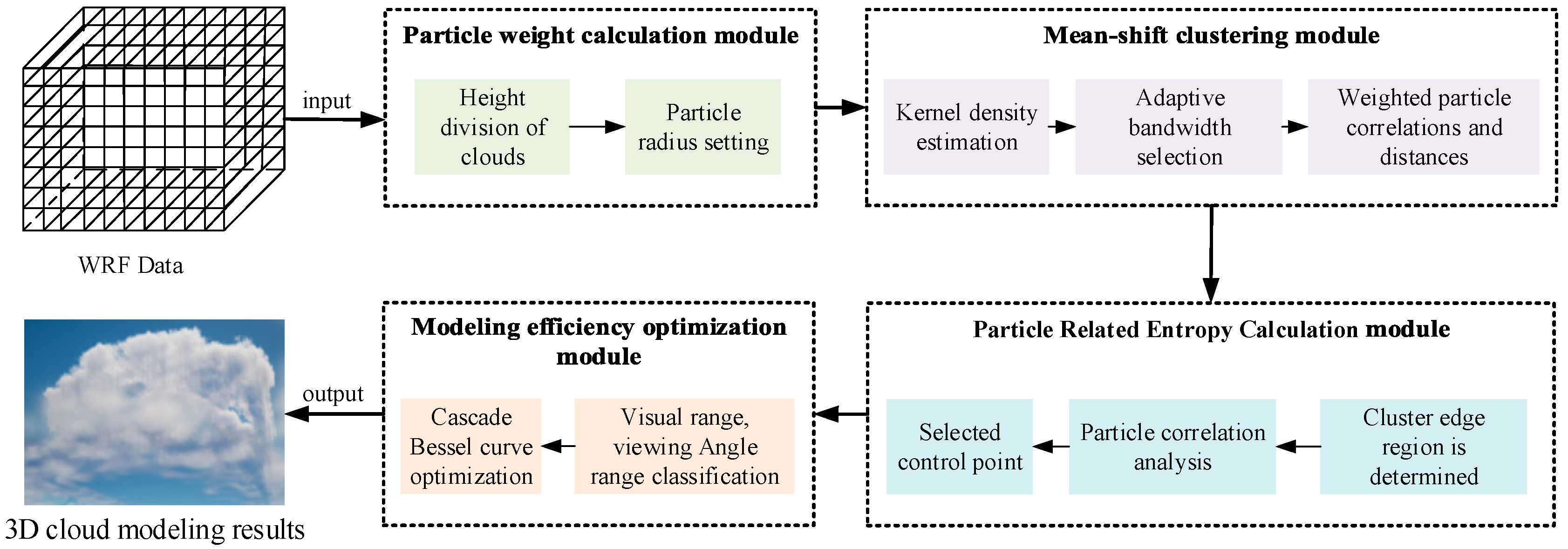
To accurately display the characteristics of cloud layers at different heights and achieve efficient modeling at long distances, we propose a multi-level particle system cloud modeling algorithm based on WRF, which combines a weight mechanism and PID controller to extract differentiated features of cloud layers. Meanwhile, the multi-scale mean-shift clustering method is utilized to accurately characterize the contours of dense cloud clusters. On this basis, we designed an optimal control point selection mechanism and utilized cascaded Bezier curves to achieve realistic long-range modeling effects while considering computational costs. The algorithm mainly consists of several parts: a particle weight calculation module, clustering module, particle correlation entropy calculation module, and modeling optimization module based on cascaded Bessel functions. The overall process is shown in Figure 1.
In Figure 1, the particle weight calculation module mainly achieves differentiated modeling of clouds at different heights through weight and particle radius settings. The clustering module adopts an adaptive multi-scale mean-shift clustering algorithm, which integrates AKDE into the mean-shift algorithm to enable adaptive bandwidth selection and accurately delineate the hierarchical structure of clouds at different altitudes, significantly improving the sense of hierarchy between clouds. The particle correlation entropy calculation module mainly determines the importance of particles in the whole based on the correlation analysis experiment between particles, and selects the optimal control point to lay a foundation for the subsequent efficiency optimization. Finally, the modeling optimization module based on cascaded Bessel functions utilizes cascaded Bessel curve technology to effectively solve the problem of high computational costs in long-range modeling while maintaining the visual effects of the model.

2.1. Particle Weight Calculation

Clouds at different heights exhibit diverse forms and state characteristics. For example, the lower cloud layer below 2000 m is mainly dominated by cumulus clouds. Clouds in this height range are evenly distributed, usually presenting a pure white color, and have relatively high cloud water content; clouds between 2000 m and 7000 m are mainly high cumulus clouds, forming relatively thin cloud layers that exhibit layered, patchy, or feathery characteristics; clouds between 7000 m and 13,000 m are mainly high-level clouds, presenting a filamentous form.
To improve the modeling accuracy, it is necessary to conduct correlation analysis within each particle cluster and screen out particles with a higher importance as candidate control points. Additionally, height information can be added to the WRF data, thereby enhancing the representation accuracy of cloud structures. However, in general, the data output by WRF does not directly provide altitude information. To obtain true altitude information, we use the conversion equation between air pressure and altitude to convert the air pressure data in WRF data to the corresponding altitude. The conversion equation is as follows:
H = 44,300 ( 1 ( p p 0 ) 1 5.256 )
where H is the height of the poster, p 0 is atmospheric pressure, and p is the current altitude pressure.
To better reflect the characteristics of cloud layers, we consider the differences in features between cloud layers at different heights and set a different particle radius for each height range. According to the height classification characteristics of cloud layers, particles with a radius range of less than 100 um are used for clouds below 2000 m to better simulate the microstructure of lower cloud layers. For clouds between 2000 and 7000 m, due to the more complex morphology and characteristics of cloud layers, particles with a radius range of 100–200 um can better simulate the particle distribution and structure of mid-level clouds. For high-level clouds above 7000 m, particles with a radius greater than 200 um are used because the clouds are often composed of larger ice crystals. Combining the cloud water mixture ratio and cloud ice mixture ratio in WRF data, the particle radius weights are set as follows:
P = e k i q i + e k w q w
where k i and k w are parameters that are adjusted according to height; q w and q i represent the cloud water mixing ratio and cloud ice mixing ratio, respectively.
The three-dimensional particle system processed by assigning particle weights may experience systematic errors in specific scenes, such as when a certain value of the cloud ice mixture ratio or cloud water mixture ratio is too large or too small. To solve this problem, this article uses a PID controller for error control. The PID controller mainly consists of three parts—a proportional term, integral term, and differential term—which can be used to quickly and accurately adjust the parameters of the particle system in the dynamic process of 3D cloud modeling, thereby minimizing system errors.
o u t p u t = p ( 1 + k p e + k i e   d t + k d d e d t )
where o u t p u t represents the result; k p represents the proportional term, which reflects the degree of influence of the current error on the controller output; k i represents the integral term, which is used to handle the system static error, that is, the error that the system cannot completely eliminate; k d represents the differential term, which is used to suppress the system oscillation and improve the system response speed.

2.2. Mean-Shift Clustering

In the process of cloud modeling, cloud layers are typically composed of cloud patches with varying densities. The mean-shift clustering algorithm, being a non-parametric clustering algorithm based on density, aligns well with the requirements of cloud modeling, especially when capturing cloud clusters in regions of higher density. However, the existing mean-shift clustering algorithm performs poorly when it comes to modeling multi-level structures. To address the complex and variable multi-level structures of cloud layers, we extend mean-shift clustering to a multi-scale approach and integrate the AKDE method to achieve dynamic clustering, thus better accommodating the multi-level structures within cloud layers. Our algorithm effectively preserves the hierarchical features of cloud layers at different altitudes, ensuring both the visual stability and authenticity of clouds even in the scenes of long-range modeling. The iterative process of mean-shift clustering is illustrated in Figure 2.
Given that WRF data are three-dimensional, in order to more accurately estimate local density, we use a three-dimensional kernel function for density estimation, as shown in (4).
f ( x ) = 1 n h 3 i = 1 n K ( x x i h )
where n is the number of samples, h represents bandwidth, and K ( ) is the three-dimensional Gaussian kernel function; the equation is shown in (5).
K ( u ) = 1 ( 2 π ) 3 2 e ( u 2 2 )
Employing a three-dimensional Gaussian kernel function offers a superior means of illustrating the spatial distribution features of three-dimensional data, precisely capturing the arrangement of points within the dataset in three-dimensional space. Equation (6) displays the gradient formula for kernel density estimation in three-dimensional Euclidean space, utilizing the mean-shift clustering algorithm.
f h , k ( x ) = 2 c k , d n h 5 [ i = 1 n K ( x x i h 2 ) ] [ i = 1 n x i K ( x x i h 2 ) i = 1 n K ( x x i h 2 ) x ]
where c k , d is the normalization constant. According to (6), the vector of the mean-shift clustering algorithm can be represented as follows:
m h , G ( x ) = i = 1 n x i K ( x x i h 2 ) i = 1 n K ( x x i h 2 ) x
The centroid iteration position of the mean-shift clustering algorithm can be obtained by (7). For sample points in three-dimensional Euclidean space, the next centroid position is shown as (8).
C j + 1 = m h , G ( x ) + x = i = 1 n x i K ( x x i h 2 ) i = 1 n K ( x x i h 2 )
Due to the significant impact of bandwidth on the performance of mean-shift clustering, dynamically selecting bandwidth to achieve optimal performance during the mean-shift clustering process is an urgent problem. To solve this problem, our algorithm combines mean-shift clustering with AKDE, enabling the mean-shift algorithm to achieve adaptive bandwidth selection based on local density changes in the cloud. Specifically, considering the bandwidth value as a representation correlated with cloud density, adaptive bandwidth adjustment is achieved by locally estimating the density of each grid point and mapping the density to the bandwidth using a linear function. The AKDE formula is shown in (9).
ρ ( x i ) = j = 1 k 1 x i x j
where x i and x j represent data points, and ρ ( x i ) represents the local density at the point x i . With the local density data of all grid data points obtained, the mapping function equation is shown in (10).
b w ( x , y ) = x = 1 , y = 1 n k ( c ¯ ( x , y ) ) n
where b w ( x , y ) is the adaptive bandwidth of the current cluster, c ¯ ( x , y ) represents the local density value at the centroid of the cluster, and k ( ) represents the linear function mapping the local density value to the bandwidth value, and the linear function equation is represented as follows:
k ( c ¯ ( x , y ) ) = c ¯ ( x , y ) ( ρ max ρ min )
where ρ max and ρ min respectively represent the maximum and minimum local density values within the current data range. This strategy can more flexibly adapt to the data characteristics of different density regions, enabling more accurate reflection of local density changes when simulating cloud layers, and thus capturing the density distribution inside the cloud layer more finely.
Due to the excessive reliance on local distance information and the lack of consideration for the correlation between particle attributes in the AKDE algorithm, this paper introduces a mechanism for weighted calculation of particle correlation and Euclidean distance between particles in the clustering process. This mechanism ensures that the importance of each particle attribute is fully considered during the clustering process, while using Euclidean distance weighting to compensate for the shortcomings of the AKDE algorithm in dealing with distant particles, ensuring that the clustering results are more authentic and accurate. The weighting equation between x i = ( x i 1 , x i 2 , x i 3 , , x i d ) and x j = ( x j 1 , x j 2 , x j 3 , , x j d ) is shown in (12).
D ( x i , x j ) = x i x j = k = 1 d ω k | x i k x j k | 2
where d is the total number of particles, x i k and x j k represent the value of each particle for the k -th attribute, and ω k represents the weight of the k -th attribute. The coefficient selection for weighted calculation is determined by the influence of the attributes themselves on the cloud formation process. For example, attributes such as particle size and color have a greater impact on cloud modeling, while particle velocity has a smaller impact. Therefore, the weighting coefficient of the former is greater than that of the latter.
The mean-shift algorithm finds the maximum value of local density by iterating, so it may be severely affected by algorithm efficiency when processing large-scale 3D data. To address this issue, we adopt a strategy of reducing the computation of particles with high similarity to minimize the number of iterations. Firstly, assuming that the number of particles in each cluster is the same, the modeling can be achieved by finding the minimum number of available particles required in all clusters. Therefore, the probability of finding at least one available particle in each cluster is shown in (13).
p = C N min 1 M 1 C N min + M 1 M 1 = ( N min 1 ) ! N min ! ( N min M ) ! ( N min + M 1 )
where M represents that there are M clusters in the dataset, and N min represents the minimum number of available particles required to find all clusters. Therefore, when N min > > M , all clusters can be found. In the actual modeling process, adjusting the number of clusters according to the size of the dataset and finding the minimum number of available particles required for all clusters can achieve efficient clustering.

2.3. Particle-Related Entropy Calculation

In the actual modeling process, changes in LoS have a significant impact on modeling accuracy and efficiency. Especially when the LoS becomes farther, the use of traditional particle modeling methods often leads to excessive consumption of computational resources. This is because the modeling method of using a fixed particle number and radius is difficult to adapt to changing observation conditions. In addition, changes in observation angles also lead to dynamic changes in particle importance information, further exacerbating the complexity of modeling. Therefore, we refine the calculation of particle-related entropy into two levels: intra-cluster and inter-cluster, aiming to reduce unnecessary particle calculations and optimize the calculation process. When implementing particle-related entropy calculation within a cluster, the focus is on particles near the cloud edge contour, while optimizing other particles within the cluster using a linear dilution strategy. This processing method ensures that when the LoS changes, the contour of the cloud can be optimized based on the edge contour particle information, and the integrity of the internal structure of the cloud can be ensured based on the density within the cluster, thereby ensuring modeling accuracy and improving computational efficiency.
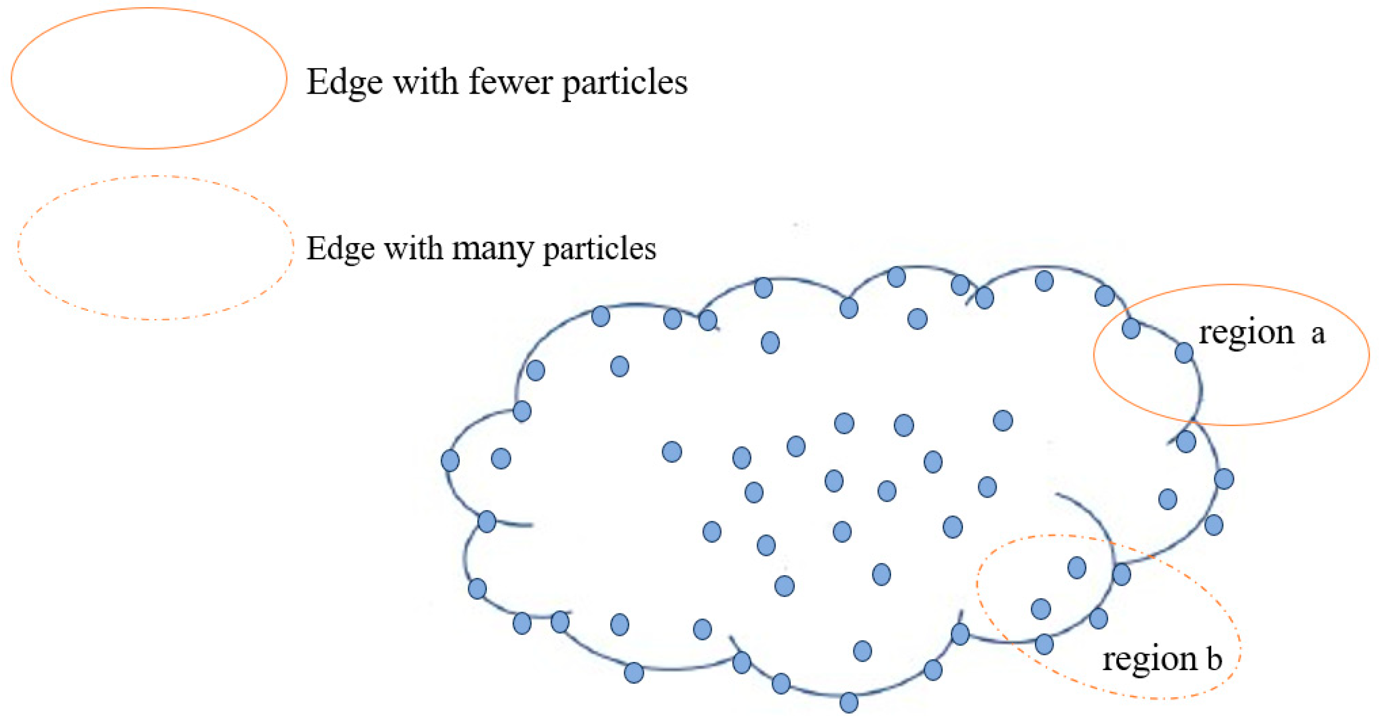
When calculating particle-related entropy within a cluster, the primary focus is on accurately identifying particles within the cluster boundary to reduce the computational complexity of unnecessary particles. Therefore, we utilize the density-based mean-shift clustering algorithm to define edge regions by identifying areas with a low density or significant density gradients, where edge particles are often distributed. In Figure 3, all particles in the edge region of the cloud are shown, while only a portion of particles in the center region are displayed, mainly highlighting the contour-related features of particles in the edge region.
There is a significant difference in the complexity of line segments and the number of control points between region a and region b, which makes their roles in cloud optimization different. Region b has more contour control points, which are more important for cloud contour. To ensure uniform selection of cloud edge control points, the number of control points should be positively correlated with the density of the edge region. For example, in region b, which has higher density, more control points should be selected than in region a.
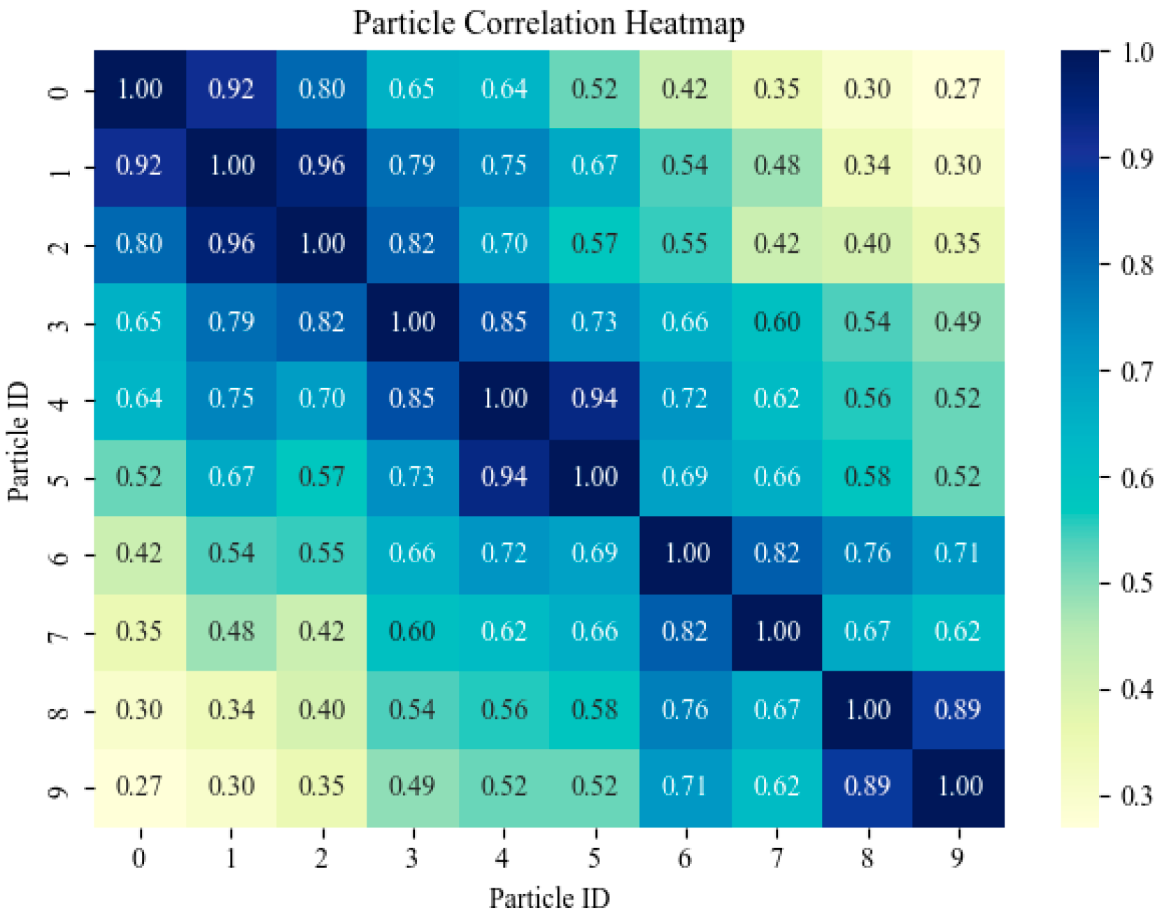
In 3D cloud modeling, the importance of cloud particles lies in their correlation with the overall cloud, that is, to what extent cloud particles can represent the information of the cloud as a whole. In the evaluation of the importance of cloud particles to the overall cloud, most existing methods directly perform inter-particle correlation analysis. Considering the multitude of particle attributes, this process is extremely cumbersome. Therefore, we introduce the concept of particle correlation entropy, which maps the multidimensional attributes of cloud particles to a one-dimensional array in the form of a linked list, thereby simplifying the computational complexity of inter-particle correlation. This process collects time series data, including key attributes such as position, velocity, color, and particle radius, and normalizes them to ensure data consistency and comparability.
In order to accurately analyze the importance of cloud particles in the overall cloud, it is necessary to perform relevant entropy calculations. Considering the advantages of a low computational complexity, high robustness, and powerful linear and nonlinear data processing capabilities of the Maximum Information Coefficient (MIC), we choose the MIC algorithm for correlation analysis and conduct correlation entropy calculation within the cluster. As mentioned earlier, edge particles play an important role in cloud contour characterization. Therefore, in this paper, edge particles are extracted one by one, and their importance in the overall cloud is evaluated by calculating the average entropy of each edge particle and other edge particles. The average correlation entropy is calculated as follows:
x i = j = 1 n 1 M ( x i , x j ) n 1
where M ( x i , x j ) represents the correlation coefficient between x i and x j , and n is the total number of particles. After obtaining the average correlation entropy of each important particle, the setting of the correlation entropy mean threshold is the key to determining the classification of particle importance. Therefore, we conduct error experiments on different threshold settings for high-level cloud regions, and uses cloud modeling error calculation to quantitatively evaluate and analyze the rationality of the threshold value range. The error equation for cloud modeling is shown in (15):
R E = i = 1 k ρ ( x i ) j = 1 n ρ ( x j )
where R E represents the error for cloud modeling, k represents the number of particles greater than the threshold, n is the total number of particles, and ρ ( ) represents the local density of the particle. By calculating the ratio between the total density of particles exceeding the threshold and the overall density, we can determine the size of the error, as demonstrated in the correlation analysis experiment in Section 3.2.1.

2.4. Modeling Optimization Based on Cascaded Bessel Functions

To fully utilize the importance information of boundary particles, we propose a cascaded Bezier curve based on the Bezier curve, selecting 2° and 30 px as thresholds for changes in viewing angle and LoS. We select the number of edge control points within each LoS range based on particle density, to achieve a cloud contour representation under different LoSs and viewing angles. Moreover, in long-range scenes, sparse processing of particles within cloud layers significantly reduces computational burden. This method can solve the problem of wasted computing resources at different viewing distances while ensuring the realism of 3D clouds.
Firstly, the visual range is divided into 100–150 px, 400–450 px, and 600–650 px, representing three observation levels: near, medium, and far. Each observation level has different requirements for the specific shape of clouds, such as requiring more cloud details for close range observation, while focusing more on the overall shape of clouds for long-range observation. Therefore, appropriate polynomial fitting methods are determined based on different observation levels to obtain the relationship between particle position and attribute information. Here, we use the least squares method to construct a fitting formula, as shown in (16):
f ( x ) = a 0 + a 1 x + a 2 x 2 + + a n x n
where f ( x ) is the fitted curve, n represents the order, and the minimum residual sum of squares can be obtained using the following equation:
i = 1 m ( y i f ( x i ) ) 2
where m represents the length of the dataset, and y i represents the particle correlation information. The coefficient solution of the least squares method can be achieved through matrix operations, and its coefficient matrix is the Vandermonde matrix, as shown in (18):
1 x 1 x 1 2 x 1 n 1 x 2 x 2 2 x 2 n 1 x m x m 2 x m n
where n represents the order, and m represents the length of the dataset. The coefficient vector is [ a 0 , a 1 , , a n ] Τ a and the observation vector is [ y 0 , y 1 , , y m ] Τ . The solution of the least squares method is obtained by solving the linear equation system A Τ A a = A Τ y , where A is the Vandermonde matrix, a is the coefficient vector, and y is the observation vector. According to the experimental results, it was found that using n = 11 , n = 7 , and n = 5 for polynomial fitting is the best for the three LoS ranges of 100–150 px, 400–450 px, and 600–650 px, respectively.
After establishing the intrinsic correlation between particle position and its attribute information, the next focus of research is on how to adaptively determine the number of control points in the cloud edge region within each LoS range. Therefore, we adjust the number of control points based on the cloud density distribution and particle importance information at different LoSs, so that the larger the LoS, the fewer the control points. Subsequently, based on the adjusted number of control points, the order of the Bezier curve is adjusted accordingly to optimize the modeling efficiency. Specifically, this algorithm uses linear interpolation to configure control points, to achieve a centralized allocation of computing resources in high-density areas. The linear interpolation is shown in (19):
n = n 1 + ( d d 1 ) ( n 2 n 1 ) d 2 d 1
where d 1 and d 2 are the density of known points and distributed at both ends of the current point, n 1 and n 2 are the number of control points for d 1 and d 2 , respectively, a is the density of the current point, and n 
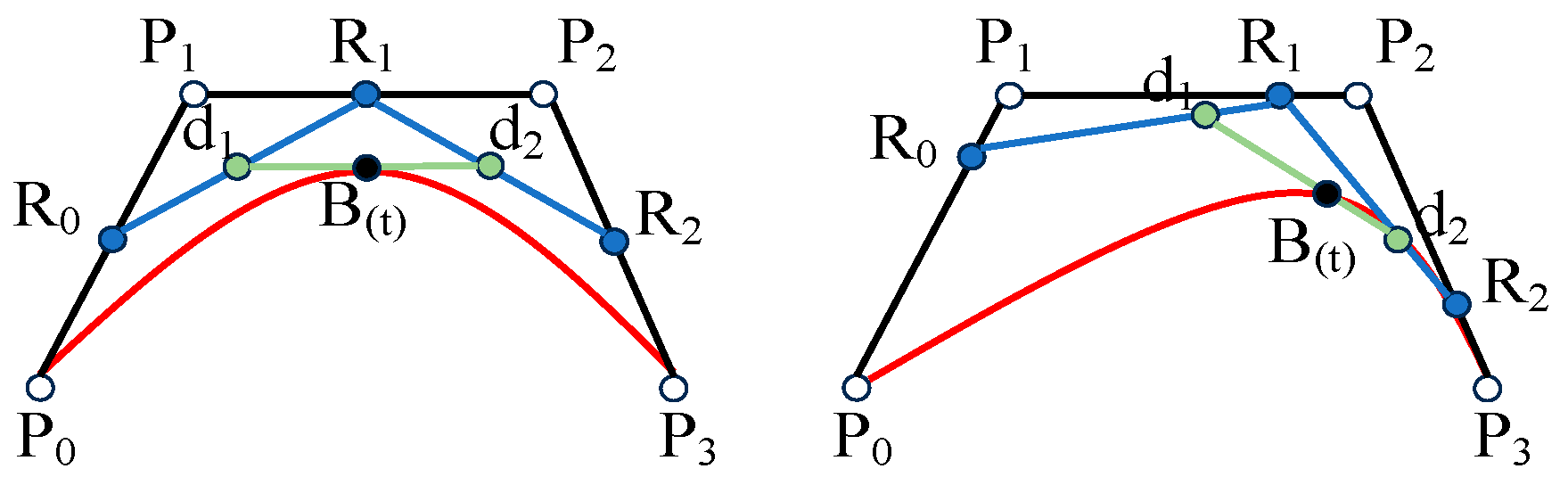
is the number of new control points obtained, and the position of the control points is adjusted. The number of control points in the local space determines the order of the Bezier curve. For example, when there are four control points, a third-order Bezier curve is used for optimization. The third-order Bezier curve is shown in Figure 4.
b n ( t ) = b 0 n ( t ) = j = 0 n b j B j n ( t )
where n represents the order of the Bezier curve, b n ( t ) represents a point on the curve, b j represents a control point, and B j n ( t ) represents a Bernstein polynomial; the Bernstein polynomial is shown in (21):
B i n ( t ) = n t t i ( 1 t ) n i
where B i n ( t ) is a Bernstein polynomial with t [ 0 , 1 ] . By utilizing the unique characteristics of Bezier curves, it is possible to significantly reduce computational costs while preserving the contour of the curve.

3. Experiment and Analysis

3.1. Experimental Setup and Experimental Scheme

The experimental equipment has an Intel (R) Core (TM) i9-10900X processor (Portland, OR, USA), 32 GB of memory, NVIDIA GeForce GTX 2080Ti GPU (Santa Clara, CA, USA), and an Ubuntu 18.04 operating system (Cape Town, South Africa). We select different 3D cloud data under two weather conditions, tropical cyclone and sea fog, as the initial WRF data. In the two sets of WRF data, cloud1 represents cumulus clouds below 2000 m in tropical cyclone weather, cloud2 represents high cumulus clouds between 2000 and 7000 m in tropical cyclone weather, cloud3 represents convective clouds above 7000 m in tropical cyclone weather, cloud4 represents stratus clouds below 2000 m in sea fog weather, cloud5 represents high cumulus clouds between 2000 and 7000 m in sea fog weather, and cloud6 represents convective clouds above 7000 m in sea fog weather. The experimental data parameter configuration is shown in Table 1.
To verify the superiority of our algorithm in modeling performance and visual representation in this paper, we conducted correlation analysis experiments, cloud modeling visual effect experiments, and cloud modeling efficiency experiments on the two WRF datasets. In addition, our algorithm has been validated under tropical cyclone and sea fog conditions, as these scenarios feature typical, complex, and rapidly evolving cloud systems that are particularly challenging for modeling. Its applicability to more extreme phenomena such as hurricanes remains theoretical at this stage. Future work will involve further experiments to comprehensively assess performance under highly dynamic meteorological conditions.

3.2. Experimental Result

To accurately evaluate the efficiency and quality of cloud modeling results, this experiment selected running time, particle count, visual effects, and other evaluation indicators, and conducted comparative experiments under different particle counts, LoS ranges, and weather types.

3.2.1. Correlation Analysis Experiment

To accurately evaluate the critical role of particles in cluster edge regions in cloud overall modeling optimization, this experiment used the coefficient of mutual information (MIC) method to analyze the correlation of key particles in edge regions at different heights. Through error experiment analysis, appropriate thresholds were set to determine the importance of particles in the cloud overall. To visually demonstrate the experimental results, this experiment specially drew correlation information heat maps for a typical region, as shown in Figure 5. This region represents a high-level cloud with extremely sparse particle density, with 10 particles.
After obtaining the correlation analysis results of particles in the high-level cloud region, the mean operation was performed on them, as shown in (15). Based on the mean value, a threshold range was set to conduct cloud modeling error experiments. The larger the value, the better its performance. The results are shown in Table 2.
Table 2 shows that when the threshold is set to 0.8 and 0.9, the representativeness of the obtained particles to the whole is poor. However, when the threshold is set to 0.7 or 0.6, the overall effect is significantly improved. The difference between the threshold set to 0.7 and the threshold set to 0.6 is relatively small compared to the whole, but the computational cost when the threshold is set to 0.7 is much smaller than when the threshold is set to 0.6. Therefore, in this study, 0.7 is selected as the threshold for particle importance judgment.

3.2.2. Cloud Modeling Efficiency Experiment

To comprehensively evaluate the modeling efficiency improvement effect of our algorithm within the conventional LoS range, and verify the advantages of the algorithm in saving computational costs as the observation LoS gradually increases, the efficiency experiments of cloud modeling were conducted at different observation distances and heights. Due to the poor performance of most particle algorithms in large-scale cloud scenes, we selected three algorithms with outstanding performance among similar algorithms, including Particle Systems based on Cellular Automata (PSCA) [16], Particle Systems based on Levels of Detail (PSLOD) [22], and Particle Systems based on Leonard Jones Potential (PSLJP) [23], for comparison.
Firstly, under the condition of an LoS range of 100–150 px, a comparison of cloud modeling efficiency was conducted on clouds of different heights under two weather types: tropical cyclone and sea fog. The experimental results are shown in Table 3 and Table 4, with bold indicating the optimal data.
From Table 3, it can be observed that when the cloud type is cloud1, the running time of our algorithm is reduced by 37.0% compared to the best performing particle system based on detail level among similar algorithms. When the cloud type is cloud2, the running time of our algorithm is reduced by 33.3% compared to the best performing PSLJP among similar algorithms. When the cloud type is cloud3, the running time of our algorithm is reduced by 23.8% compared to the best performing PSLJP among similar algorithms.
From Table 4, it can be observed that when the cloud type is cloud1, the proposed algorithm reduces the running time by 24.3% compared to the best performing particle system based on detail level among similar algorithms. When the cloud type is cloud2, our algorithm reduces the running time by 20.7% compared to the best performing PSLJP among similar algorithms. When the cloud type is cloud3, our algorithm reduces the running time by 16.7% compared to the best performing PSLJP among similar algorithms.
In summary, when the LoS range is 100–150 px, our algorithm shows varying degrees of improvement in cloud modeling efficiency at different heights and levels compared to three similar algorithms under two weather types. The lower the cloud height, the greater the performance advantage of our algorithm. This is because under different LoSs, our algorithm is based on the actual situation in clustering. We combine ADKE for adaptive bandwidth calculation and reduce the computational load by reducing some particles with high similarity.
However, the above experiments did not demonstrate the computational efficiency advantage of our algorithm compared to similar excellent algorithms when the LoS changes. Therefore, for the two LoS ranges of 400–450 px and 600–650 px, our algorithm and three excellent algorithms of the same kind will be compared in modeling efficiency for different types of clouds under different weather types, and corresponding experimental analysis will be conducted. Since the cloud modeling effect also changes when the LoS changes, it is not suitable to simply judge the cloud modeling efficiency based on running time. Therefore, this experiment will use the visual effect of the PSCA as the benchmark and use the number of particles to reflect the cloud modeling efficiency when the visual effect is basically the same. The results of the particle number comparison experiment are shown in Table 5, and the bold data are the optimal data.
From Table 5, it can be observed that when the LoS range is 400–450 px and 600–650 px, our algorithm uses significantly fewer particles than similar algorithms while ensuring visual effects. Different cloud types under different weather conditions in the 400–450 px LoS range are displayed using line charts, as shown in Figure 6 and Figure 7.
In Figure 6 and Figure 7, it can be observed that within the visual range of 400–450 px and with a tropical cyclone weather type, when the cloud type is cloud1, the particle count used in our algorithm is reduced by at least 37.90% compared to the other three similar algorithms. When the cloud type is cloud2, our algorithm uses at least 34.17% fewer particles compared to the other three similar algorithms. When the cloud type is cloud3, our algorithm uses at least 18.97% fewer particles compared to the other three similar algorithms. When the cloud type is cloud1 within the visual range of 400–450 px and the weather type is sea fog, our algorithm reduces the number of particles used by at least 13.83% compared to the other three similar algorithms. When the cloud type is cloud2, our algorithm uses at least 10.28% fewer particles compared to the other three similar algorithms. When the cloud type is cloud3, our algorithm uses at least 8.73% fewer particles compared to the other three similar algorithms.
Similarly, different cloud types under different weather conditions within the 600–650 px LoS range will be displayed more intuitively using line charts, as shown in Figure 8 and Figure 9. From Figure 8 and Figure 9, it can be observed that within the 600–650 px LoS range and with a weather type of tropical cyclone, when the cloud type is cloud1, the particle count used in our algorithm is reduced by at least 37.52% compared to the other three similar algorithms. When the cloud type is cloud2, our algorithm uses at least 37.37% fewer particles compared to the other three similar algorithms. When the cloud type is cloud3, our algorithm uses at least 28.01% fewer particles compared to the other three similar algorithms. When the cloud type is cloud1 within the 600–650 px LoS range and the weather type is sea fog, our algorithm reduces the number of particles used by at least 21.58% compared to the other three similar algorithms. When the cloud type is cloud2, our algorithm uses at least 13.74% fewer particles compared to the other three similar algorithms. When the cloud type is cloud3, our algorithm uses at least 10.74% fewer particles compared to the other three similar algorithms.
In summary, our algorithm demonstrates superior performance in modeling low clouds and under long sightlines, particularly in complex scenarios such as tropical cyclones. This advantage stems from its ability to identify high-importance particles near cloud contours and refine cloud geometry via cascaded Bessel functions. Quantitatively, compared to the three baseline methods [16,22,23], our algorithm reduces particle usage by up to 37.90% in tropical cyclone scenes and 21.58% in sea fog scenes (Figure 6, Figure 7, Figure 8 and Figure 9), while maintaining comparable or better visual fidelity. These results indicate significantly improved computational efficiency. Moreover, by adaptively adjusting particle allocation across vertical layers, our method maintains structural coherence and detail retention with fewer resources—an improvement not achieved in prior studies, where uniform particle distribution often leads to either under-sampling or redundancy in sparse cloud regions.

3.2.3. Cloud Vision Comparison Experiment

According to the results of the cloud modeling efficiency experiment, compared with the other three algorithms, our algorithm reduced the running time of the algorithm by up to 60.1% at most and by an average of 37.5%. Particles numbers were reduced by up to 64.3% at most and by an average of 30.1%. In ensuring modeling efficiency, it reduced the calculation cost. At the same time, it can be observed from this experiment that the algorithm proposed in this paper can maintain the contour shape and stratification continuity of clouds within different altitude ranges well, and that it and has a better performance than the other three algorithms in terms of the authenticity of the cloud structure.
In this study, modeling experiments were conducted for three distinct types of cloud layers under representative and complicated meteorological conditions: tropical cyclone and sea fog. Cloud1: stratocumulus clouds below 2000 m; cloud2: clouds between 2000 and 7000 m; cloud 3: cumulus clouds above 7000 m. Comparisons were made with three other excellent algorithms of the same kind. When the viewing distance range is 100–150 px, the experimental comparison diagram is shown in Figure 10.
According to Figure 10, our method demonstrates clearer cloud structures and higher visual fidelity across cloud1, cloud2, and cloud3. In terms of contour preservation, it accurately restores natural cloud boundaries, with smooth transitions especially in cloud2 and cloud3, whereas PSCA and PSLJP exhibit blurred or broken edges. Regarding detail retention, the proposed method performs particularly well in cloud3, maintaining microstructures even in sparse high-altitude regions, while PSCA shows noticeable structural loss. Overall, our method ensures consistent spatial structure and visual realism across layers, better supporting photorealistic rendering compared to PSLOD and others.
To demonstrate that our algorithm solves the problem of wasted computing resources while ensuring no significant differences in the overall contour of the cloud when the LoS increases, modeling experiments were conducted on cloud1, cloud2, and cloud3. When the viewing distance range is 600–650 px, the experimental comparison diagram is shown in Figure 11.
According to Figure 11, our method outperforms the three comparison methods within the 600–650 px viewing range. In terms of visual realism, it maintains appropriate volumetric transparency and natural light–shadow transitions in sparse high-altitude clouds, better reflecting realistic illumination effects. In contrast, PSCA and PSLJP exhibit excessive blurring or uneven brightness in this region, which undermines perceptual realism. For structural coherence, our method preserves complete cloud contours and spatial continuity, even in low-density regions. In terms of detail retention, our method captures fine feather-like structures and layered textures with smooth edge transitions and no noticeable artifacts, while PSLJP and PSCA suffer from over-smoothing and overexposure, leading to significant loss of detail.
The experimental results of cloud modeling efficiency show that the modeling efficiency of our algorithm is superior to the compared algorithms under LoS conditions, and the farther the LoS, the more prominent the optimization effect. This is because our algorithm is based on the importance of cloud particles at the edge of the cloud contour, selects the optimal control points, and uses cascaded Bessel functions to optimize the cloud contour, thereby significantly improving modeling efficiency while maintaining the modeling effect. Our algorithm also adopts the strategy of finding the minimum number of available particles for each cluster during clustering, effectively reducing the computational load of high-similarity particles. The results of cloud vision comparison experiments show that our algorithm can accurately present cloud features and their hierarchical sense at different heights under different weather types, and can effectively maintain the overall shape of clouds when optimizing long-range modeling. This is because our algorithm fully considers the physical characteristics of clouds, sets weights and selects particle radius based on cloud height, and uses PID controllers to control shape, thus solving the problem of single cloud features. On the basis of the mean-shift clustering algorithm, AKDE is introduced to achieve adaptive capture of cloud density distribution, effectively improving the hierarchical performance of clouds. Therefore, our algorithm outperforms the comparative algorithms in terms of cloud feature presentation and long-range modeling efficiency at different heights.

4. Conclusions

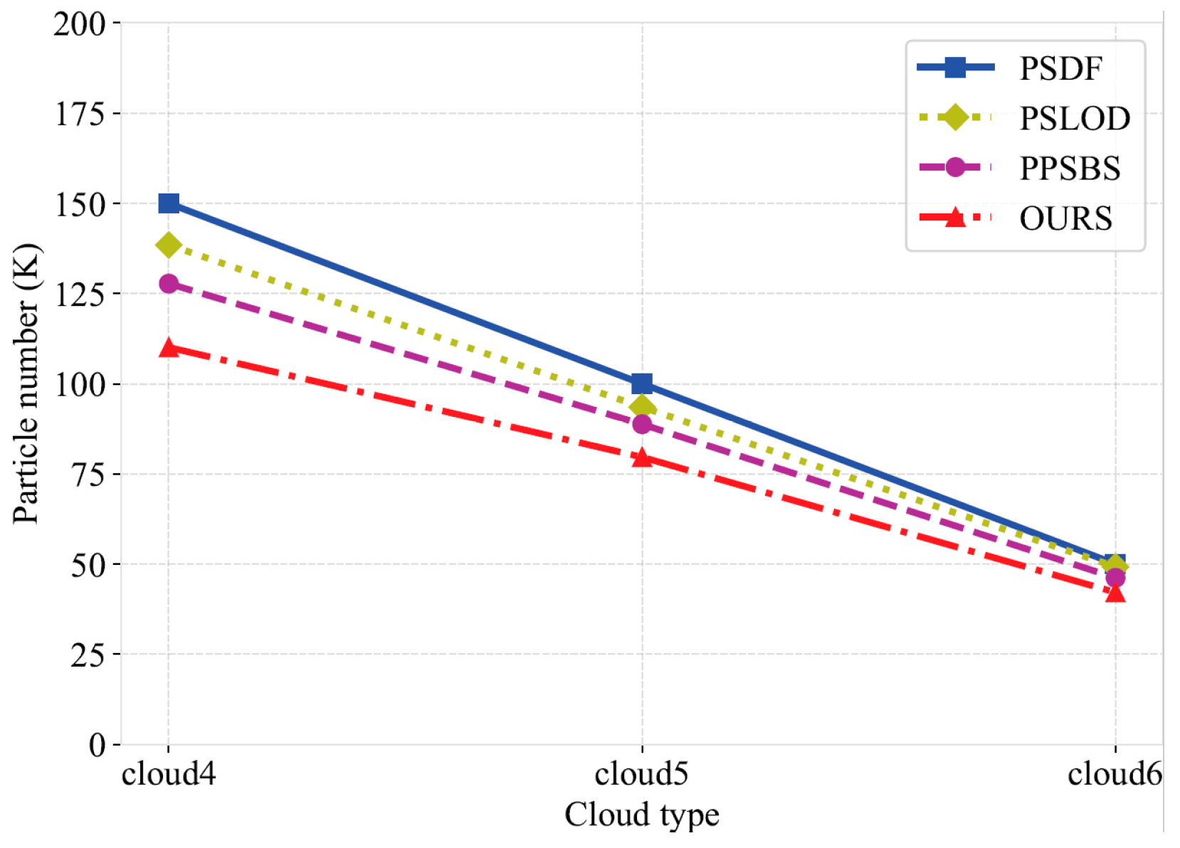
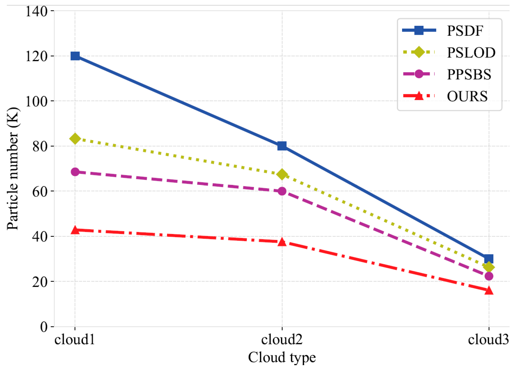
In this work, we propose a multi-level particle system 3D cloud modeling algorithm based on a WRF model to address the problem of current cloud modeling methods generally ignoring the differences in cloud characteristics at different heights and the high computational cost of remote modeling. First, we proposed a particle radius weight adjustment mechanism and a PID feedback mechanism based on the microphysical properties of clouds to enhance the differences in cloud structures at different altitudes. Secondly, based on the mean-shift algorithm, we introduced AKDE and designed a particle weighting and clustering strategy with an adaptive bandwidth to accurately capture the cloud density distribution and improve the hierarchical modeling performance. Finally, based on the correlation between the particle density in the edge region and the cloud contour, we carefully selected the optimal control points, and further improved the modeling efficiency through the cascade Bezier curve optimization under different viewing distances. The experimental results show that compared with similar algorithms, the running time of our algorithm is smaller by up to 60.1% at most and by an average of 37.5%, indicating enhanced computational efficiency and real-time capability. The number of particles is smaller by up to 64.3% at most and by an average of 30.1%, effectively reducing the calculation cost for long-range scenes. However, it should be noted that the module developed in this study has only been tested under specific meteorological phenomena, namely tropical cyclones and sea fog conditions, as these represent typical and complex weather scenarios that pose significant challenges for cloud modeling and visualization. We are also aware that when dealing with small-scale scenes, the improvement in the modeling efficiency of our algorithm is not significant, which to some extent limits its wide application in the field of cloud scene modeling. Therefore, future research will focus on improving the performance of the algorithm in small-scale scenes, further verifying it under a wider range of weather scenes, and actively exploring other potential modeling optimization strategies, with a view to further improving and expanding the application scope of this algorithm.

Author Contributions

Methodology, R.G.; Validation, J.C.; Resources, X.M.; Writing—original draft, B.W.; Writing—review & editing, L.T.; Supervision, S.Y. All authors have read and agreed to the published version of the manuscript.

Funding

Scientific and Technological Innovation 2030—“New Generation Artificial Intelligence” Major Project 2021ZD0102100.

Institutional Review Board Statement

Not applicable.

Informed Consent Statement

Not applicable.

Data Availability Statement

Data is contained within the article.

Conflicts of Interest

Julong Chen, Bin Wang, Rundong Gan, Xuepeng Mou, and Shiping Yang are employees of China Southern Power Grid (China). Ling Tan serves as a technical advisor within China Southern Power Grid (China). This study was not directly funded by the company. The company had no role in the design of the study; in the collection, analysis, or interpretation of data; in the writing of the manuscript; or in the decision to publish the article. The paper reflects the views of the scientists and not the company.

Abbreviations

The following abbreviations are used in this manuscript:
WRFWeather Research and Forecasting model
PIDProportional-Integral-Derivative controller
AKDEAdaptive Kernel Density Estimation
3DThree-Dimensional
YSUYonsei University
RRTMRapid Radiative Transfer Model
MICMaximal Information Coefficient
LoSLine-of-Sight
PSCAParticle Systems based on Cellular Automata
PSLODParticle Systems based on Levels of Detail
PSLJPParticle Systems based on Leonard Jones Potential

References

  1. Chen, G.; Wang, W.C.; Bao, Q.; Li, J. Evaluation of simulated cloud diurnal variation in CMIP6 climate models. J. Geophys. Res. Atmos. 2022, 127, e2021JD036422. [Google Scholar] [CrossRef]
  2. Chertock, A.; Kurganov, A.; Lukáčová-Medvid’ová, M.; Spichtinger, P.; Wiebe, B. Stochastic Galerkin method for cloud simulation. Part II: A fully random Navier-Stokes-cloud model. J. Comput. Physic. 2023, 479, 111987. [Google Scholar] [CrossRef]
  3. Deng, Y.; Yang, J.; Yin, Y.; Cui, S.; Zhang, B.; Bao, X.; Chen, B.; Li, J.; Gao, W.; Jing, X. Quantifying the spatial inhomogeneity of ice concentration in mixed-phase stratiform cloud using airborne observation. Atmos. Res. 2024, 298, 107153. [Google Scholar] [CrossRef]
  4. Burrows, S.M.; McCluskey, C.S.; Cornwell, G.; Steinke, I.; Zhang, K.; Zhao, B.; Zawadowicz, M.; Raman, A.; Kulkarni, G.; China, S.; et al. Ice-nucleating particles that impact clouds and climate: Observational and modeling research needs. Rev. Geophys. 2022, 60, e2021RG000745. [Google Scholar] [CrossRef]
  5. Gao, Z.; Xiang, J. Real-time 3D object detection using improved convolutional neural network based on image-driven point cloud. Recent Adv. Electr. Electron. Eng. 2021, 14, 826–836. [Google Scholar] [CrossRef]
  6. Zhang, C.; Xu, M. Time-segment photovoltaic forecasting and uncertainty analysis based on multi-objective slime mould algorithm to improve support vector machine. IEEE Trans. Power Syst. 2023, 39, 5103–5114. [Google Scholar] [CrossRef]
  7. Di Paola, F.; Cimini, D.; De Natale, M.P.; Gallucci, D.; Gentile, S.; Geraldi, E.; Larosa, S.; Nilo, S.T.; Ricciardelli, E.; Ripepi, E.; et al. Wind Speed Downscaling of the WRF Model at Sub-Kilometer Scale in Complex Terrain for Wind Power Applications. IEEE J. Sel. Top. Appl. Earth Obs. Remote Sens. 2024, 17, 9139–9177. [Google Scholar] [CrossRef]
  8. Liu, W.; Xue, Y.; Ling, X.; Gao, J.; Tang, Z.; Wu, S.; He, B. Estimation Of Regional Air Pollution In Xuzhou City Based On WRF-Chem Model. In Proceedings of the IGARSS 2023–2023 IEEE International Geoscience and Remote Sensing Symposium, Pasadena, CA, USA, 16–21 July 2023; IEEE: Piscataway, NJ, USA, 2023; pp. 3846–3849. [Google Scholar] [CrossRef]
  9. Agrawal, N.; Das, A.; Modani, M. Scalability analysis of weather research forecast model on nvidia ampere based dense gpu cluster. In Proceedings of the 2022 International Conference on Computing, Communication, Security and Intelligent Systems (IC3SIS), Kochi, India, 23–25 June 2022; IEEE: Piscataway, NJ, USA, 2022; pp. 1–6. [Google Scholar] [CrossRef]
  10. Solano-Farias, F.; Ojeda, M.G.V.; Donaire-Montaño, D.; Rosa-Cánovas, J.J.; Castro-Díez, Y.; Esteban-Parra, M.J.; Gámiz-Fortis, S.R. Assessment of physical schemes for WRF model in convection-permitting mode over southern Iberian Peninsula. Atmos. Res. 2024, 299, 107175. [Google Scholar] [CrossRef]
  11. Ma, M.; Tang, J.; Ou, T.; Zhou, P. High-resolution climate projection over the Tibetan Plateau using WRF forced by bias-corrected CESM. Atmos. Res. 2023, 286, 106670. [Google Scholar] [CrossRef]
  12. Merino, A.; García-Ortega, E.; Navarro, A.; Sánchez, J.L.; Tapiador, F.J. WRF hourly evaluation for extreme precipitation events. Atmos. Res. 2022, 274, 106215. [Google Scholar] [CrossRef]
  13. Tao, C.; Fu, S.; Qi, J.; Li, H. Thick cloud removal in optical remote sensing images using a texture complexity guided self-paced learning method. IEEE Trans. Geosci. Remote Sens. 2022, 60, 5619612. [Google Scholar] [CrossRef]
  14. Zhang, S.; Yuan, G.; Wang, B. Optimization Methods for Real-time Volumetric Cloud Simulation. In Proceedings of the 2023 3rd International Conference on Consumer Electronics and Computer Engineering (ICCECE), Guangzhou, China, 6–8 January 2023; IEEE: Piscataway, NJ, USA, 2023; pp. 31–35. [Google Scholar] [CrossRef]
  15. Morrison, H.; van Lier-Walqui, M.; Fridlind, A.M.; Grabowski, W.W.; Harrington, J.Y.; Hoose, C.; Korolev, A.; Kumjian, M.R.; Milbrandt, J.A.; Pawlowska, H.; et al. Confronting the challenge of modeling cloud and precipitation microphysics. J. Adv. Model. Earth Systems 2020, 12, e2019MS001689. [Google Scholar] [CrossRef] [PubMed]
  16. Roy, S.; Das, S. Clouds in the basins of fully asynchronous cellular automata. Adv. Complex Syst. 2022, 25, 2250013. [Google Scholar] [CrossRef]
  17. Wang, T.; Xu, Y.; Li, R.; Wang, H.; Xiong, Y.; Wang, X. Simulating hyperelastic materials with anisotropic stiffness models in a particle-based framework. Comput. Graph. 2023, 116, 437–447. [Google Scholar] [CrossRef]
  18. Cai, H.; Yang, Y.; Chen, Q. Distribution characteristics of cloud types and cloud phases over China and their relationship with cloud temperature. Remote Sens. 2022, 14, 5601. [Google Scholar] [CrossRef]
  19. Yang, D.; Zhou, W.; Seidel, S.D. Substantial influence of vapour buoyancy on tropospheric air temperature and subtropical cloud. Nat. Geosci. 2022, 15, 781–788. [Google Scholar] [CrossRef]
  20. Zhang, Z.; Zhang, Y.; Li, Y.; Liang, X. Cumuliform cloud animation control based on natural images. In Proceedings of the 2020 International Conference on Virtual Reality and Visualization (ICVRV), Recife, Brazil, 13–14 November 2020; IEEE: Piscataway, NJ, USA, 2020; pp. 218–224. [Google Scholar] [CrossRef]
  21. Zhang, J. Implementation and optimization of particle effects based on unreal engine 4. In Proceedings of the 5th Annual International Conference on Information System and Artificial Intelligence [ISAI2020], Zhejiang, China, 22–23 May 2020; IOP Publishing: Bristol, UK, 2020; 1575, p. 012187. [Google Scholar] [CrossRef]
  22. Xie, Y.; Kou, X.; Li, P. A simulation method of three-dimensional cloud over WRF big data. EURASIP J. Wirel. Commun. Netw. 2019, 2019, 252. [Google Scholar] [CrossRef]
  23. Elhaddad, A.; Elhaddad, F.; Sheng, B.; Zhang, S.; Sun, H.; Wu, E. Real-time cloud simulation using lennard-jones approximation. In Proceedings of the 29th International Conference on Computer Animation and Social Agents, Geneva, Switzerland, 23–25 May 2016; pp. 131–137. [Google Scholar] [CrossRef]
Figure 1. The overall framework diagram of the algorithm in this paper.
Atmosphere 16 00571 g001
Figure 2. Mean-shift clustering iteration principle diagram.
Atmosphere 16 00571 g002
Figure 3. Diagram of cloud particle contour correlation in edge region.
Atmosphere 16 00571 g003
Figure 4. Third-order Bezier curve. Where B ( t ) is a point on the curve, P 0 is the starting point, P 1 and P 2 are the first and second control points, respectively, P 3 is the ending point, t [ 0 , 1 ] , and the Bezier curve is shown in Equation (20).
Atmosphere 16 00571 g004
Figure 5. Correlation heatmap of 10 particles within high-level cloud region.
Atmosphere 16 00571 g005
Figure 6. Particle numbers under tropical cyclone weather within visual range of 400–450 px.
Atmosphere 16 00571 g006
Figure 7. Particle numbers under sea fog weather within visual range of 400–450 px.
Atmosphere 16 00571 g007
Figure 8. Particle numbers under tropical cyclone weather within visual range of 600–650 px.
Atmosphere 16 00571 g008
Figure 9. Particle numbers under sea fog weather within visual range of 600–650 px.
Atmosphere 16 00571 g009
Figure 10. Comparison of cloud modeling effects with visual range 100–150 px. (a) Cloud modeling effects under tropical cyclone weather; (b) cloud modeling effects under sea fog weather.
Atmosphere 16 00571 g010
Figure 11. Comparison of cloud modeling effects with visual range 600–650 px. (a) Cloud modeling effects under tropical cyclone weather; (b) cloud modeling effects under sea fog weather.
Atmosphere 16 00571 g011
Table 1. WRF physical and dynamical settings.
CategoryParameterValue
Spatial SettingsLength and Width (km)150
Longitude and Latitude Range30–36 N, 116–122 E
Grid Spacing (km)3
Number of Vertical Levels50
Physical SchemesMicrophysics SchemeThompson Scheme
Cumulus Convection SchemeKain–Fritsch Scheme
Planetary Boundary Layer SchemeYSU Scheme
Land Surface ModelNoah Land Surface Model
Longwave Radiation SchemeRRTM Scheme
Shortwave Radiation SchemeDudhia Scheme
Temporal SettingsSimulation Period00:00 UTC 1 August 2024–00:00 UTC 2 August 2024
Spin-up Period6 h
Time Step15 s
Table 2. Cloud modeling error estimation under different threshold selections.
SceneT = 0.9T = 0.8T = 0.7T = 0.6
high-level cloud region0.700.780.880.89
Table 3. Running time of various algorithms in tropical cyclone with sight range 100–150 px.
MethodCloud1Cloud2Cloud3
PSCA (ms)1586233
PSLOD (ms)1004825
PSLJP (ms)1254521
Our algorithm (ms)633216
Table 4. Running time of various algorithms under sea fog weather with visual range 100–150 px.
MethodCloud1Cloud2Cloud3
PSCA(ms)955129
PSLOD(ms)743226
PSLJP(ms)812918
Our algorithm(ms)562315
Table 5. Comparison of particle numbers.
SightlineMethodCloud1Cloud2Cloud3Cloud4Cloud5Cloud6
400–450 pxPSCA (k)1501005015010050
PSLJP (k)125.4986.4848.52138.4793.5249.21
PSLOD (k)110.3572.6943.28127.7588.7846.17
Ours (k)68.5247.8535.07110.0879.6542.14
600–650 pxPSCA (k)12080301208030
PSLJP (k)83.2767.4426.25102.0575.4028.25
PSLOD (k)68.5459.9622.3195.7770.0125.22
Ours (k)42.8237.5516.0675.1060.3922.85
Disclaimer/Publisher’s Note: The statements, opinions and data contained in all publications are solely those of the individual author(s) and contributor(s) and not of MDPI and/or the editor(s). MDPI and/or the editor(s) disclaim responsibility for any injury to people or property resulting from any ideas, methods, instructions or products referred to in the content.

