An Efficient Deep Learning Method for Typhoon Track Prediction Based on Spatiotemporal Similarity Feature Mining

Abstract

Typhoon is one of the most destructive natural disasters, and it affects human society significantly. To reduce the negative impacts, many deep learning models for predicting future typhoon tracks have appeared. However, most of these models use all of the data they obtain as input, which may cause the diversity of typhoon tracks to have a negative impact on the prediction outcomes. In this paper, a joint method is proposed. The method mainly includes two parts: First, use a spatiotemporal similarity feature mining model to find out paths that are similar to the ongoing typhoon. Second, a deep learning model for processing sequence data is trained by these similar paths and then used for predicting the future track points’ latitude and longitude. The joint method bridges the gap in deep learning models’ ability to process spatial information and the shortcomings of spatiotemporal similarity feature mining models in predicting future data. In the experiment, we use a spatiotemporal similarity feature mining model to generate different input datasets by changing the number of similar paths in it, which can compare the model’s accuracy in different inputs. Also, real typhoon data recorded in the North West Pacific Ocean are used in the experiment. Through a comparison between the real path and prediction results in longitude and latitude, we find that 100–250 similar typhoon tracks as input have the best prediction effect in different tasks and are more accurate in long-term prediction.

1. Introduction

A tropical storm is a low-pressure vortex with warm structure, and its name is usually determined by the location of the ocean from which it forms. Typhoons form in the northwest Pacific Ocean and the South China Sea. Similar tropical storms that form in the northeast Pacific Ocean and the Atlantic Ocean are called hurricanes. When it comes to the Indian Ocean, the tropical storms are often referred to as cyclones [1,2]. Typhoon, hurricane, and cyclone all have powerful destructive abilities and cause much loss to the countries and regions affected by them. In recent years, typhoon Doksuri in 2023 stands out as a major typhoon event. It triggered severe flooding and geological disasters across the Beijing–Tianjin–Hebei area, China, impacting millions and resulting in substantial economic losses. A total of 154 people were killed in this disaster [3]. The losses from the typhoon in China from 2014 to 2024 (except 2020, 2021, and 2022) recorded by the Chinese Civil Affairs Statistical Yearbook [4,5,6,7,8,9,10,11] are shown in

Table 1. Losses caused by typhoons in China from 2014 to 2024 (except 2020, 2021, and 2022).

Year	Affected Population	Dead Person (Including Missing)	Collapsed Houses	Damaged Houses	Direct Economic Loss
2014	2659.5	111	5.2	52.6	693.4
2015	2375.6	57	2.3	27.1	684.2
2016	1721.2	198	3.7	18.1	766.4
2017	587.9	44	0.4	3.8	346.2
2018	3260.6	83	2.4	20.5	697.3
2019	1484.4	#	1.5	13.3	#
2023	1131.6	12	0.7	#	474.9
2024	1153.6	18	0.3	19.5	853.4

Units: 10,000 people, people, 10,000 rooms, 10,000 rooms, 100 million yuan; ‘#’ means the data are not found.

. The data in the table shows that the losses caused by typhoons are immense. In 2024 alone, typhoons caused direct economic losses of 85,340 million yuan. Simultaneously, it also affects multiple ecological components in wetlands, including plants and animals, carbon and nitrogen cycling, water quality, and other critical factors [12]. Such a great economic loss not only affects people’s lives but also increases the pressure on the country’s finances. Therefore, it is extremely necessary to create and update the method for predicting future typhoon tracks based on the historical path data.

In the field of typhoon track prediction, the traditional method is called the Numerical Weather Prediction Model (NWP). NWP uses physics, fluid dynamics, and thermodynamics equations to forecast future weather based on atmospheric processes [13]. The innovative method employs deep learning. It boasts the capabilities of handling large-scale data, possessing powerful feature learning abilities, enjoying wide applicability, and making predictions based on time-series data [14]. The typhoon historical path data are a kind of trajectory data, also it has a very distinct time series feature. It means most of the methods based on deep learning can predict the future track by fitting and regression. To predict time-series data effectively, some commonly used models are RNN [15], LSTM [16], CNN-LSTM [17], and Conv-LSTM [18]. The first two models solely rely on time-series data as input, whereas the Conv-LSTM model needs image data, transforming the original temporal computations into image processing. However, most of the studies used all of the historical path data as the input. This results in a substantial increase in model training time, and often the outcomes obtained are not optimal.

NWP models and deep learning methods all have advantages and disadvantages in predicting typhoon tracks. NWP predicts typhoons by simulating the physical mechanisms of the atmosphere-ocean coupling process. It not only has physical interpretability but also possesses the ability to predict extreme events. However, NWP models require vast data as input and exhibit inherent limitations in forecasting typhoons, which are mesoscale weather systems and rapidly changing meteorological conditions [19,20]. Deep learning methods for time-series data focus on fitting the target curve, relying more on the statistical properties and pattern recognition capabilities of the data, without necessarily requiring numerous natural factors as parameters. It enables more efficient data utilization and fully uncovers hidden linear and nonlinear features [21]. However, it fails to reflect the physical significance of the data and has relatively poor responsiveness to extreme events.

This paper mainly studies deep learning methods to predict and decrease the amount of input data, at the same time, reduce time costs and increasing the accuracy of prediction results. The sea–atmosphere interaction is not considered in this research. Deep learning models are data-driven approaches that implicitly capture physical processes rather than explicitly constructing mechanisms like sea–atmosphere interactions, differing fundamentally from physics-based modeling paradigms. In our experiments, typhoon parameters, like center pressure and intensity, are adopted as inputs, which inherently encode indirect signatures of oceanic influences. For example, sea surface temperature variations manifest through pressure-intensity dynamics. Our study focuses on achieving efficient prediction using readily available meteorological variables, as direct data acquisition for sea–atmosphere interactions remains observationally intensive and computationally burdensome, thereby running counter to the study’s objectives of operational efficiency and practical feasibility. We can choose the data input into the deep learning model to find the optimal fitting effect. Using deep learning methods to predict the typhoon track is still a developing research field. From the initial proposal by Rita et al. to use Artificial Neural Networks (ANNs) for processing satellite imagery data to predict cyclone paths [22], to the using of Long Short-Term Memory (LSTM) networks that consider both short-term and long-term information for more accurate path predictions [23], and then to the adoption of Conv-LSTM methods, which combine convolutional image processing with LSTM neural networks for typhoon path prediction [24]. Each step has used novel and effective deep learning strategies at that time to reach a high level of accuracy. Although deep learning methods are still developing, it has already shown great potential in meteorology and climate forecasting.

To find out the best input for the deep learning model, we should conduct a similarity analysis on typhoon trajectories. Several methods have been employed to analyze typhoon similarity, like RDP [25], FCM [26], and SA_DBN [27]. In this paper, a machine learning method is introduced as a spatiotemporal similarity feature mining model. Dynamic Time Wrapping (DTW) is an algorithm that can measure the similarity between two time series of data [28]. The smaller the warping distance obtained from the DTW calculation between two time series, the more similar the two time series are [29]. It is widely used in speech recognition, handwriting recognition, and other time series analysis fields. As mentioned above, historical typhoon data are a kind of time series data. Under the same geographic coordinate system, we can conduct DTW similarity analysis on all the coordinate points along two typhoon paths [30]. After obtaining the similarity scores, we can select typhoon data within a certain threshold range or a specific number of typhoons as the input data. Then, these data will be input into an LSTM model for training.

The rest of this paper is organized as follows: Section 2 mainly describes the method of using LSTM and DTW to predict the path of a typhoon. After training and predicting steps, we obtain the result of the model and use a real typhoon to evaluate the effectiveness of this method in Section 3. In Section 4, we discuss the further investigation and disadvantages of this method. Finally, we conclude this paper in Section 5.

2. Methodology and Data Preprocessing

This section delineates the methodological framework and data preprocessing procedures employed in the study. We provide a comprehensive overview of the analytical techniques, computational algorithms, and data refinement protocols that underpin the research design. An LSTM model will be proposed in this section, playing a role in predicting future data. The method’s corresponding flowchart is illustrated in Figure 1.

2.1. Spatiotemporal Similarity Feature Mining Model

The similarity analysis model used in this method is DTW. This section will briefly propose the DTW algorithm, demonstrate the calculation of DTW distance, and explain how DTW is utilized in this study to identify similar typhoon tracks.

2.1.1. Dynamic Time Wrapping

Dynamic Time Wrapping (DTW) is a machine learning method. It is a dynamic programming algorithm used to calculate the similarity between two time series of data [31]. This algorithm is suitable for handling situations where two time series have different lengths, such as speech recognition, handwritten font recognition, and comparing the similarity between different typhoon paths.

Now we have two different time series of data $S=\left\{s_1,s_2,\dots ,s_m\right\}$ and $Q=\left\{q1,q2,\dots ,qn\right\}$ with the length of m and n. The DTW algorithm finds an optimal path between two time series by minimizing the sum of the distances of all corresponding points on that path, thereby representing the shortest path or wrapping path between two sequences. The length of this path is commonly used as a metric for the DTW similarity between the two sequences. The shortest path is given as $P=\left\{p_1,p_2,\dots ,p_n\right\}$, means the map information generated from the two time series. Before we begin to calculate the similarity, the wrapping path must satisfy at least three constraints:

Boundary: $p_1=$ (1, 1) and $p_k=$ ($m$,$n$);

Community: Given $p_k=$ ($a$,$b$) and $p_{k-1}=$ ($a^{\prime }$,$b^{\prime }$) where $a-a^{\prime }\le 1$ and $b-b^{\prime }\le 1$;

Monotonicity: Given $p_k=$ ($a$,$b$) and $p_{k-1}=$ ($a^{\prime }$,$b^{\prime }$) where $a-a^{\prime }\ge 1$ and $b-b^{\prime }\ge 1$;

The calculation of the distance formula in the DTW algorithm is shown below:

$$DTW\left(S,Q\right)=min\sum _{k=1}^{K}d\left(p_k\right)$$

(1)

In this formula, $K\in \left[max\left(m,n\right),m+n-1\right]$ is an integer representing the length of the path. $d\left(p_k\right)$ stands for the distance between two points $s_i$ and $q_{i}i\in \left[1,m\right],j\in \left[1,n\right]$. Here $d\left(p_k\right)=d\left(i,j\right)=\left|s_i-q_i\right|$.

After the calculation of the distance, dynamic programming is used to calculate the cumulative distance $D\left(i,j\right)$ with distance $d\left(i,j\right)$ by adding the minimum cumulative distance among its three adjacent elements in the matrix: the one to the left-upper, the one above, and the one to the left. The formula is shown below:

$$D\left(i,j\right)=d\left(i,j\right)+\mathit{min}\left(D\left(i,j-1\right),D\left(i-1,j\right),D\left(i-1,j-1\right)\right)$$

(2)

where $D\left(\mathrm{0,0}\right)=0,D\left(i,0\right)=D\left(0,j\right)=$∞.

2.1.2. Using DTW Algorithm to Choose the Optimal Input of LSTM

The similarity of typhoon trajectories is predominantly determined by two key parameters: the central latitude and central longitude of the typhoon systems, which can determine the positions of typhoon track points. These geospatial coordinates serve as the primary determinants in assessing path alignment and deviation patterns during comparative analyses.

To assess typhoon track similarity, the longitude and latitude time series data of typhoon pairs are processed independently. Specifically, the DTW shortest distances are computed separately for each spatial dimension (longitude and latitude) to quantify alignment discrepancies. The decoupled computation of longitude and latitude DTW distances ensures that axial-specific temporal distortions (e.g., east–west and north–south drift patterns) are preserved, thereby capturing anisotropic path variability. Subsequently, the overall similarity metric is derived by aggregating the DTW distances from both dimensions.

A sorting utility is then employed to rank all typhoon tracks based on their ascending overall similarity scores. The top 50, 100, 250, 500, and 750 most similar typhoon tracks are extracted and exported into five distinct files, which serve as input datasets for the LSTM model. Within these output files, all trajectories are chronologically ordered, forming continuous time series sequences characterized by longitude and latitude coordinates.

In practical scenarios, complete typhoon tracks are unavailable at the initial observation stage, necessitating predictive analyses based on partial path data. To address this, our methodology employs the first 10–12 data points (corresponding to 3–4 days of trajectory records) of a target typhoon as the query sequence. This truncated sequence is dynamically aligned with all complete historical tracks using DTW to identify the most analogous paths.

As the typhoon evolves and additional positional data are recorded, the DTW-based similarity matching is iteratively recalibrated. This progressive refinement incorporates newly acquired path points, enabling adaptive updates to the optimal historical analogs for enhanced prediction accuracy.

2.2. Deep Learning Model for Processing Sequence Data

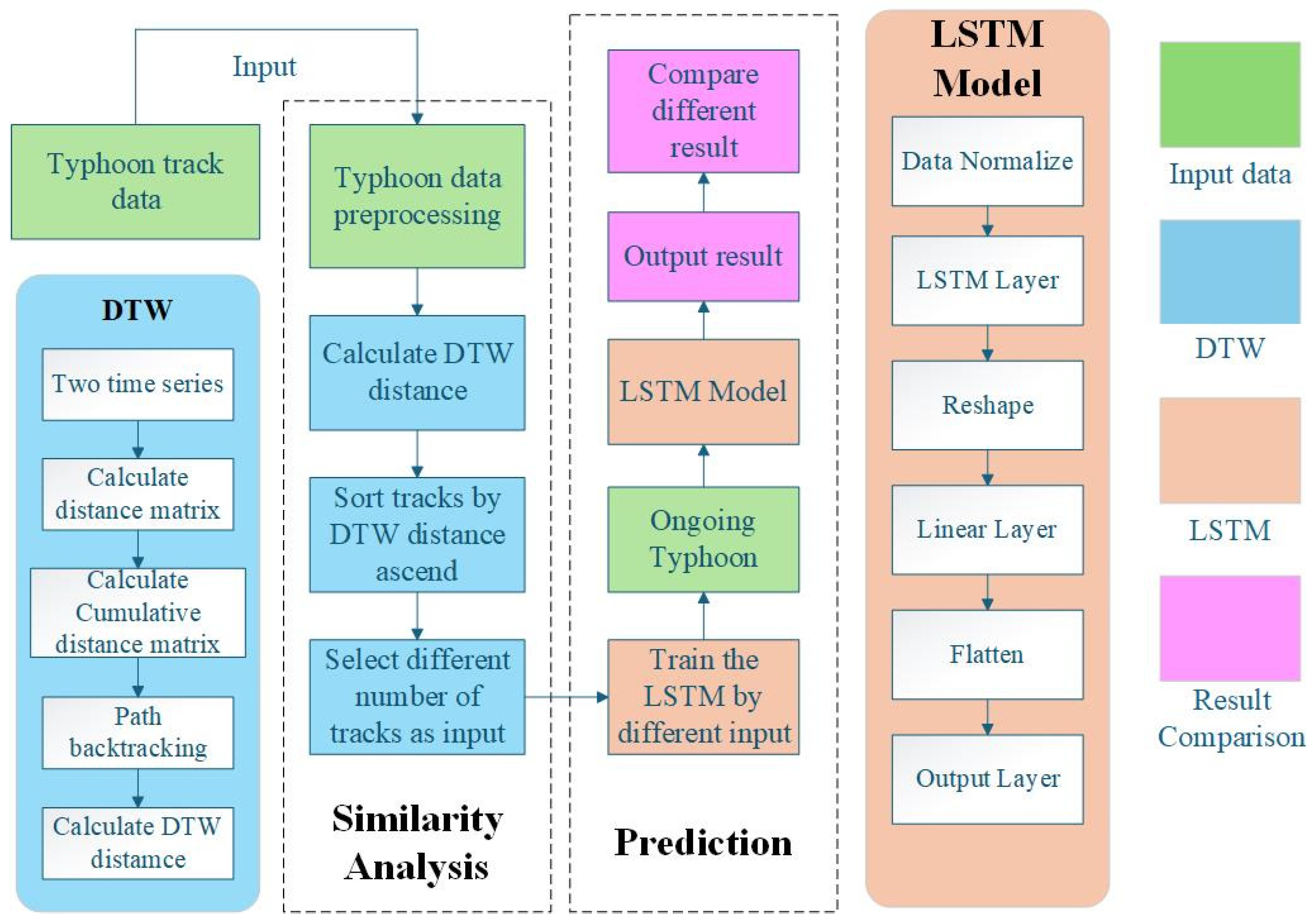
In this part, an LSTM deep learning model for processing and predicting typhoon tracks will be proposed. It learns the diverse input data provided by the similarity analysis model and predicts the real typhoon tracks in the future.

2.2.1. Long Short-Term Neural Network

A Long Short-Term Neural Network (LSTM) is a kind of Recurrent Neural Network (RNN) architecture designed to process a sequence of data and capable of learning long-term dependencies. Unlike standard RNNs, LSTMs are designed to avoid the vanishing gradient problem, which can limit the ability of conventional RNNs to learn long-term dependencies [32]. These features make LSTM a good choice to handle predicting problems with long time series data.

LSTM has three gates, which control different parts of the LSTM cell. They are forget gate $F_t\in R^{N\times H_c}$, input gate $I_t\in R^{N\times H_c}$ and output gate $O_t\in R^{N\times H_c}$. The candidate memory cell, represented as ${\tilde{C}}_t\in R^{N\times H_c}$ is crucial in determining how the LSTM’s internal memory will evolve over time, serving as a ‘proposed update’ to the cell state. The data that is utilized to inform the decisions made by the LSTM gates and to compute the candidate memory cell comprises two primary components: the input data at the current time step $X_t\in R^{N\times d}$ and the hidden state from the previous time step $H_{t-1}\in R^{N\times H_c}$. These two pieces of information work in tandem to shape the flow of data through the LSTM network and contribute to its ability to capture and retain long-term dependencies in sequential data. In this paper, we build a unidirectional LSTM network [33] for typhoon track prediction.

In the LSTM cell, the Input Gate plays a role in determining which new information from the current input and previous hidden state should be added to the cell state, ensuring that only relevant and significant data are incorporated. The Forget Gate decides what information from the previous cell state is no longer needed and should be discarded, helping the network forget irrelevant details and focus on important features. In the last, the Output Gate regulates the output of the LSTM cell, controlling which parts of the cell state should be revealed based on the current context, thus providing the network with the ability to output information that is relevant for the next step in the sequence.

The hidden states in an LSTM cell are illustrated as follows:

$$I_t=\sigma \left(X_t{W}_{xi}+{H_t}_{-1}{W}_{hi}+b_i\right)$$

(3)

$$F_t=\sigma \left(X_t{W}_{xf}+H_{t-1}{W}_{hf}+b_f\right)$$

(4)

$$O_t=\sigma \left(X_t{W}_{xo}+H_{t-1}{W}_{hc}+b_o\right)$$

(5)

$$\tilde{C}t=tanh\left(X_t{W}_{xc}+H_{t-1}{W}_{hc}+b_c\right)$$

(6)

$$C_t=F_t\mathrm{☉}{C}_{t-1}+I_t\mathrm{☉}{\tilde{C}}_t$$

(7)

$$H_t=O_t\mathrm{☉}tanh\left(C_t\right)$$

(8)

where $N$ is the batch size. $H_c$ and $d$ are the number of hidden units and features. $\sigma$ is a sigmoid activation function that ranges between 0 and 1, and the $tanh$ function is a hyperbolic tangent activation function that squashes input values to a range between −1 and 1. $\mathrm{☉}$ indicates element-wise multiplication. $W_{xi},W_{xf},W_{xo},W_{xc}\in R^{d\times H_c}$ and $W_{hi},W_{hf},W_{ho},W_{hc}\in R^{h\times H_c}$ are weight parameters and $b_i,b_f,b_o,b_c\in R^{1\times Hc}$ are biased parameters.

2.2.2. Using an LSTM Model for Future Prediction

The LSTM model is built for processing typhoon data, because the track data are kind of sequence data. Also, LSTM is commonly used in future locations of moving objects, which means it has the ability to perform space-time prediction [34]. In this paper, the deep learning model is a kind of multi-task LSTM model, which uses a network model to simultaneously predict the longitude and latitude [35].

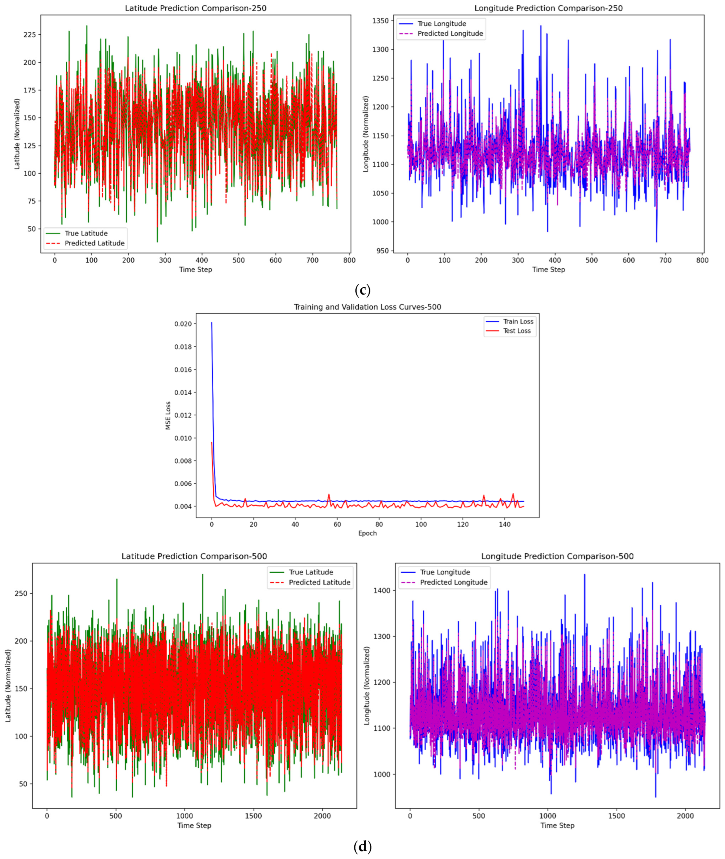
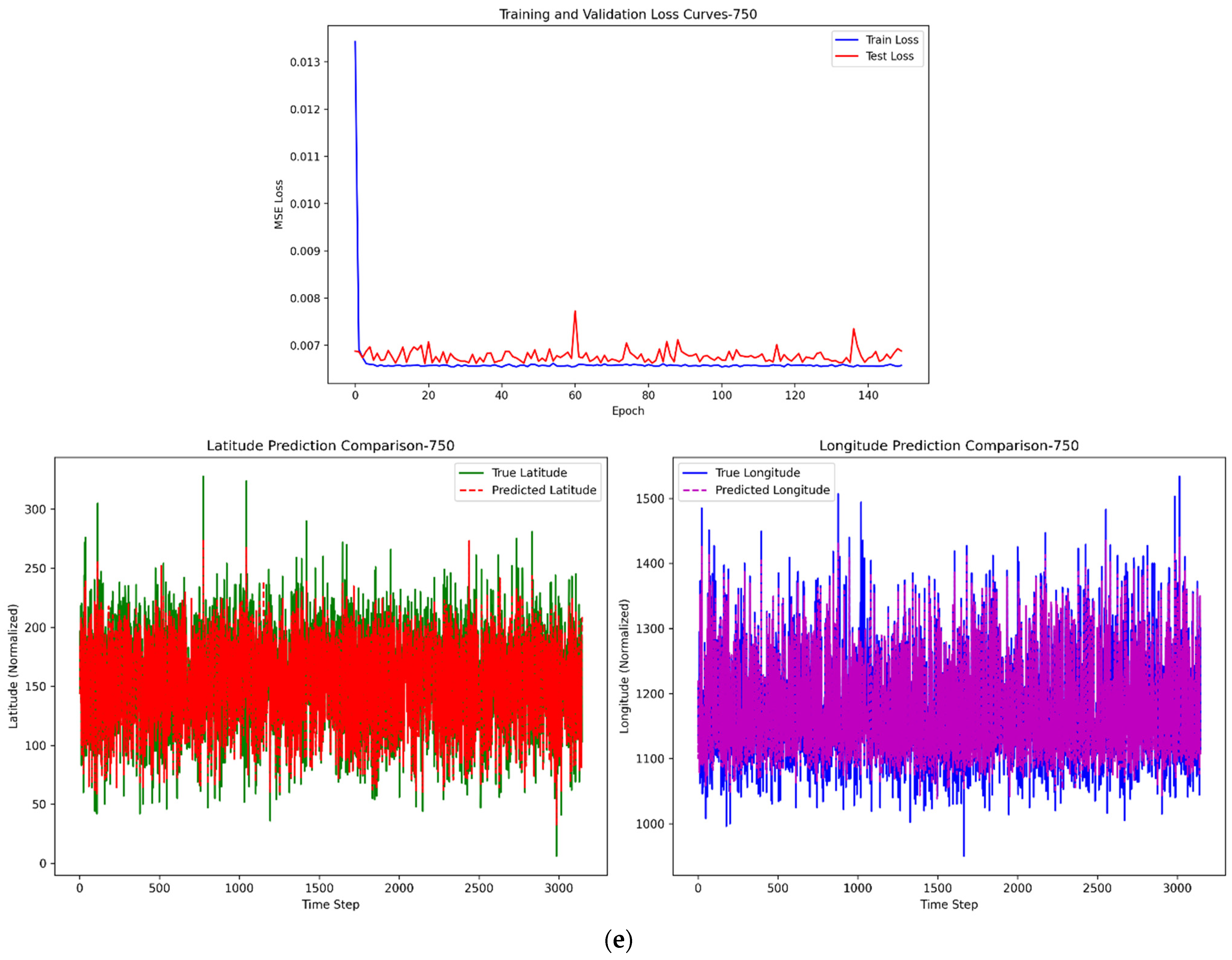
The input data to the model comprise four dimensions: typhoon intensity, central latitude, central longitude, and central pressure, which were retained during the data preprocessing phase. These variables collectively contribute to the computations within the LSTM layers, jointly determining the parameters of the hidden states and enhancing the predictive accuracy of the model. The optimal paths obtained using the DTW algorithm, comprising 50, 100, 250, 500, and 750 paths, are sequentially input into the LSTM model for training. The performance of the model is evaluated based on the results from the test set to determine the optimal number of paths. This approach allows for a systematic comparison of the model’s predictive accuracy across different path quantities, ultimately identifying the configuration that yields the highest performance in terms of typhoon trajectory prediction.

Before the data were input into the model, these numerical data, such as longitude, latitudes, can be normalized to [0,1] with the function below:

$$x^{\prime }={\displaystyle \frac{x-\mathit{min}\left(x\right)}{\mathit{max}\left(x\right)-\mathit{min}\left(x\right)}}$$

(9)

where $x$ represents the original value and $x^{\prime }$ represents the normalized value.

In this research, we design a sequence-to-sequence LSTM model that processes typhoon trajectory data and outputs predictions for each time step in the input sequence. This architecture preserves temporal resolution throughout the network, making it particularly suitable for real-time trajectory updating applications.

The model accepts 3D tensors with shape (sequence length, batch size, input size), where input size is set as 4 for latitude, longitude, pressure, wind speed, and the sequence length is set as 1.

The model generates one-step predictions through a modified output layer, producing a tensor of shape (batch size, 1, output size), where output size is set as 2, representing latitude and longitude coordinates at each future time step. In the four-step prediction, we change the shape of the tensor to (batch size, 4, output size) to directly output 4 steps ahead predictions by jointly learning from historical path sequences.

The architecture employs a two-layer stacked LSTM with hidden size, enabling hierarchical feature extraction from raw input sequences. Dropout is applied between LSTM layers to mitigate overfitting.

Then, a fully connected layer transforms the final LSTM hidden state into a flattened vector of length $outputsize\times steps$, which is then reshaped to (steps, output size) to explicitly represent multi-step predictions. In one-step prediction, “steps” is set as 1 and 4 in the four-step prediction.

To balance the learning, we choose Mean Square Error (MSE) as the loss function. The loss function is shown below:

$$MSEloss={\displaystyle \frac{1}{n}}{\sum _{i=1}^n\left(X_i-{\stackrel{\wedge }{X}}_i\right)}^2$$

(10)

where $X_i$ represents the real path trajectory’s latitude or longitude, and ${\stackrel{\wedge }{X}}_i$ represents the predicted path trajectory’s latitude or longitude. These two losses will be added with the same weight. The Adam optimizer [36] is proposed in this research to utilize for gradient adjustment in LSTM models. In Adam optimizer, a weight decay regularization term was implemented to counteract overfitting in the neural network architecture.

In the context of hyperparameter optimization, we have opted for the Bayesian optimization approach. Bayesian optimization is a method designed to efficiently explore and optimize black-box functions. It achieves this by constructing a probabilistic surrogate model, typically a Gaussian Process, to approximate the unknown function and guide the search toward its global optimum [37]. The utilization of Bayesian optimization for hyperparameter tuning not only enhances the predictive accuracy of the model but also significantly curtails the temporal expenditure associated with the optimization process.

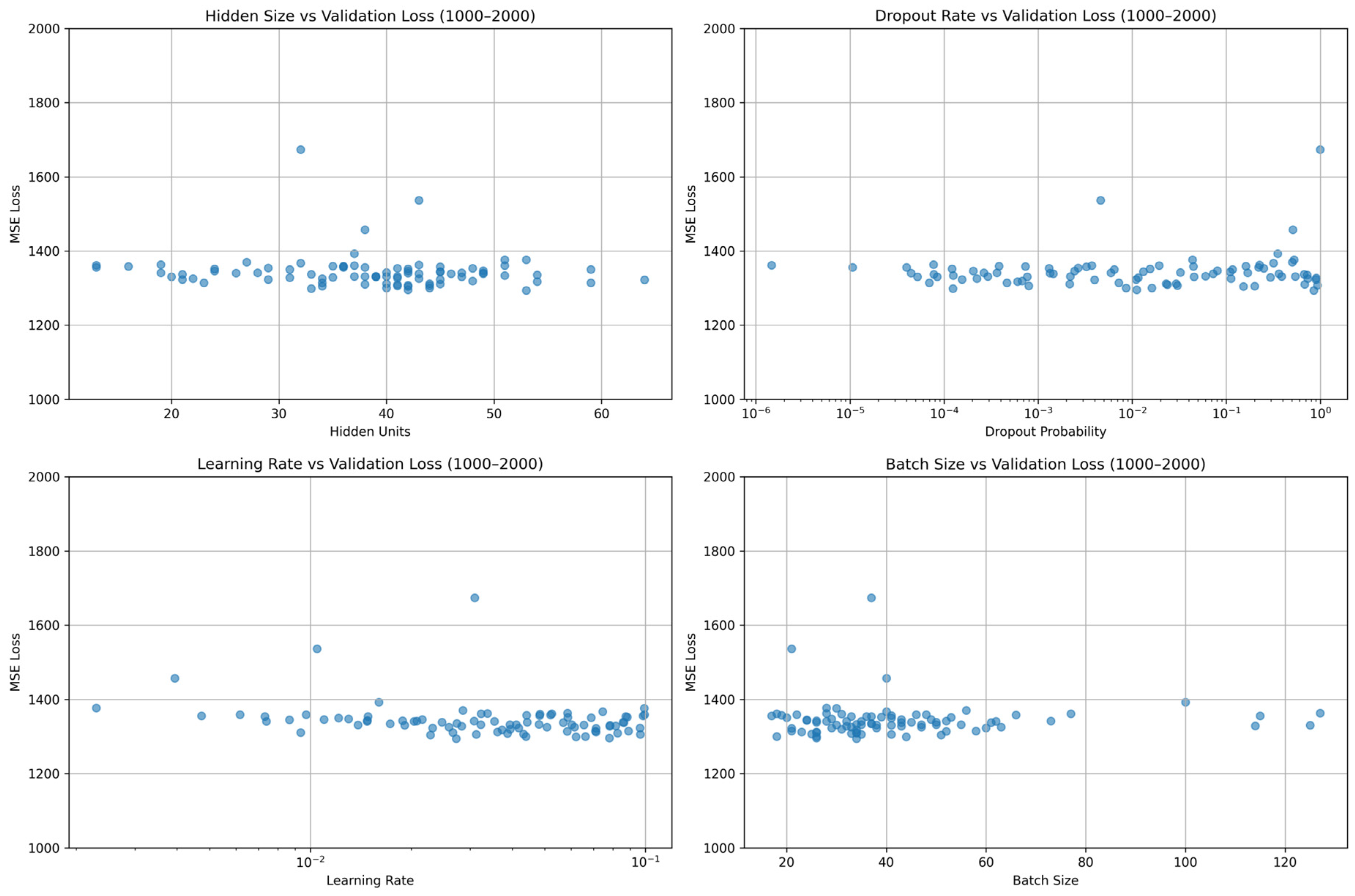
In the optimization, we allocated 70% of the dataset for training and reserved 30% for validation purposes during hyperparameter tuning. We conducted a systematic hyperparameter tuning process involving 1000 experimental trials to identify the optimal parameter configuration that minimizes the MSE on the validation dataset. The following key parameters were optimized: batch size, tested across a range of values to balance computational efficiency and gradient estimation quality. Network architecture parameters, like the number of hidden units and LSTM layers. Regularization parameters, like dropout and weight decay. In Figure 2, 100 results of the batch size, dropout, learning rate, and number of hidden units are shown, but the visualization of these results lacks controlled variable analysis, potentially obscuring the individual effects of each hyperparameter on model performance.

After Bayesian optimization, the optimal hyperparameter combination we found is as follows: the batch size is set to 26, the number of hidden units is 42, the number of LSTM layers remains at 2, the learning rate is set to 0.007, the dropout rate is set to 0.09, and the weight decay is set to 0.0004. When hyperparameters are not set to their optimal values, they can significantly impact the performance and behavior of an LSTM model. Taking the learning rate as an example, when the learning rate is either too large or too small, the longitude–direction errors in the final prediction results are substantially large. A too high learning rate can cause the optimizer to overshoot optimal minima, leading to divergent training or oscillating convergence around the minimum, resulting in suboptimal final weights. A too low learning rate, however, slows down training drastically, potentially getting stuck in flat local minima or taking impractical time to converge, and might prematurely halt at a suboptimal solution due to limited training epochs. In the realm of forecasting future data, the methodology is bifurcated into one-step prediction and four-step prediction. One-step prediction and four-step prediction both use the latest data, according to the parameters in the LSTM model, to predict for a single future time step and for four consecutive future time steps. The whole process of one-step and four-step prediction will be proposed in Section 3.

2.3. Time Series Data, Historical Typhoon Data, and Data Preprocessing

Time series refers to a sequence of numerical values of the same statistical indicator arranged in chronological order of their occurrence. These time points can be in any form of time unit, such as years, quarters, months, days, hours, etc. Time series data are widely found in numerous fields such as economics, finance, environmental science, meteorology, industrial manufacturing, and more [38]. They serve as an important tool for analyzing and predicting future trends. Historical typhoon data are information recorded in a specific chronological order, which includes details such as the geographic coordinates of the typhoon’s center, central pressure, movement speed, wind speed category, and other relevant information. Thus, typhoon data can be seen as a kind of time series data.

In this paper, the typhoon track dataset (https://data.cma.cn) adopted is real typhoon tracks. The dataset includes the typhoon track from 1949 to 2019, 6 h interval, formed in the northwest Pacific Ocean and the East China Sea, which are recorded by the China Meteorological Observatory. In this dataset, the typhoon’s name, the longitude and the latitude of the typhoon’s center, track points recorded time, central pressure, typhoon intensity, and wind speed are all recorded. Details in the dataset are shown in

Table 2. Details of the typhoon dataset.

Dataset	Typhoon
Data type	Typhoon track data
Time span	1949–2019
Num of typhoons	2389
Level of typhoon intensity	8 (level 0, 1, 2, 3, 4, 5, 6, 9)
Time interval	6 h
Latitude span	[0.5° N, 62.1° N]
Longitude span	[95° E, 202.5° E]
Pressure span	[870 hpa, 1022 hpa]

. The original data downloaded from the website are separated. We sequentially link the start of each subsequent typhoon to the end of the previous one, based on their chronological order, thereby forming a continuous and comprehensive time series.

In the context above, we have talked about the composition of the historical typhoon dataset. All of these data are organized in annual batches, with each file containing records of all typhoons within a single year. The data files spanning from 1949 to 2019 are arranged chronologically by year. However, as these data are stored as multiple discrete document files, they cannot be directly treated as a continuous time series dataset. In

Table 3. Original typhoon dataset of ‘Lekima’.

Time	Intensity	Lat (0.1° N)	Lon (0.1° E)	Prse (hpa)	Wnds (m/s)
2019080700	4	204	1281	960	38
2019080706	4	206	1277	950	44
2019080712	5	216	1270	940	50
2019080718	6	221	1264	925	55

The times are from 0:00 on 7 August 2019 to 18:00 on 7 August 2019.

, an original dataset of typhoon ‘Lekima’ is shown.

The initial step in data preprocessing involves retaining only four critical variables from the raw typhoon dataset: typhoon intensity, central latitude, central longitude, and central pressure. Extraneous metadata, such as timestamps and typhoon identifiers, are systematically pruned to reduce dimensionality and computational redundancy. The central longitude and latitude are specifically designated as pivotal input parameters for subsequent DTW algorithms. Meanwhile, all four preserved variables (typhoon intensity, latitude, longitude, and pressure) are collectively utilized as input features for the LSTM model to capture both spatial patterns and atmospheric interactions governing typhoon path evolution.

The second phase of data preprocessing entails segmenting all typhoon records into individual files utilizing the designated delimiters embedded within the dataset. This partitioning strategy is implemented to streamline subsequent DTW computations, thereby enabling efficient consolidation of aligned results into a unified output file.

Following the completion of the aforementioned data preprocessing steps, the refined dataset is now primed for integration into the two designated computational frameworks: the DTW algorithm and the LSTM model.

In this study, autocorrelation function (ACF) and partial autocorrelation function(PACF) are introduced to intuitively show the correlation of series in different lag orders, in order to determine the lag structure [39]. The calculation functions are as follows:

$$c_k={\displaystyle \frac{1}{n}}\sum _{t=1}^{n-k}\left(x_t-\overline{x}\right)\left(x_{t+k}-\overline{x}\right)$$

(11)

$$c_0={\displaystyle \frac{1}{n}}{\left(x_t-\overline{x}\right)}^2$$

(12)

$$AC{F}_k={\displaystyle \frac{c_k}{c_0}}=Cor\left(x_t,x_{t+k}\right)$$

(13)

$$PAC{F}_k=Cor\left(x_t-x_t^{k-1},x_{t+k}-x_{t+k}^{k-1}\right)$$

(14)

where $\overline{x}$ is the mean of the typhoon time series, $AC{F}_k$ and $PAC{F}_k$ are the ACF and PACF of lag order $k$. In Equation (14), $Cor\left(x_t-x_t^{k-1},x_{t+k}-x_{t+k}^{k-1}\right)$ means the correlation measure of the influence of $x_{t+k}$ on $x_t$ after removing the interference $k-1$ random variables.

3. The Experiment and Evaluation

In this paper, the typhoon track dataset (https://data.cma.cn) adopted is a real typhoon track (including the sequence of latitude, longitude, pressure, and typhoon intensity) from 1949 to 2019. The dataset encompasses a total of 2389 distinct tracks, with each successive time step separated by a 6 h interval. We set 80 percent of the input data as the training data, the remaining data are allocated as the testing data to verify the effectiveness of the model.

The prediction errors are quantified using the Mean Absolute Error (MAE) defined in Equation (15) and the Root Mean Square Error (RMSE) specified in Equation (16), which serve as key metrics to evaluate the performance and accuracy of the deep learning model.

$$MAE={\displaystyle \frac{1}{n}}\sum _{i=1}^n\left|X_i-{\stackrel{\wedge }{X}}_i\right|$$

(15)

$$RMSE=\sqrt{{\displaystyle \frac{1}{n}}\sum _{i=1}^n{\left(X_i-{\stackrel{\wedge }{X}}_i\right)}^2}$$

(16)

where $X_i$ represents the true value and ${\stackrel{\wedge }{X}}_i$ represents the predicted value.

In this experiment, the following method is used for experiment comparison:

Firstly, preprocess the raw data into a format that can be directly used for DTW calculation. From the entire dataset of typhoons, select one for prediction purposes, extract the data from its first 11 trajectory points to represent an “ongoing” typhoon track, and then remove this typhoon’s records from the preprocessed dataset. The DTW algorithm will calculate the similarity between historical data and real path data with several preceding path points to be predicted. All remaining 2388 historical typhoon tracks will undergo DTW calculations, and the resulting DTW distances will be utilized to generate input datasets with varying quantities of similar typhoons. After the DTW computation is completed, the algorithm will select 50, 100, 250, 500, and 750 similar paths as the multitask LSTM input data. After the training, these five kinds of input predictions will be compared with the real path by RMSE and MAE to evaluate the effectiveness of these input options. The training history graphs of the neural network and the comparison of accuracy on the training and test datasets for all of the input datasets are shown in Figure 3. In Figure 3, the training loss on the training set and test loss on the validation set across 150 epochs are displayed from top to bottom for scenarios using 50, 100, 250, 500, and 750 similar typhoon tracks as input, respectively, along with corresponding predictive performance validation on the test dataset. As the number of input similar tracks increases, the 20% testing set contains progressively more typhoon samples, resulting in increasingly dense data distribution in the later test sets.

Figure 4 shows the ACF and PACF plot of the typhoon time series for latitude and longitude. As we can see in the plot, we find that the ACF of latitude decays significantly more slowly than that of longitude, which is attributed to the latitude dependence of the Coriolis force [40]. It can also be observed that the ACF of longitude exhibits values less than zero, which is attributed to the oscillations in the typhoon track along the longitudinal direction. The ACFs of both longitude and latitude exhibit a trend of slow decay, indicating tailing, while their PACFs demonstrate truncation, dropping rapidly to near zero. According to the result of the ACF and PACF plots, it can be determined that the typhoon time series data follows an autoregressive model.

3.1. One Step Prediction

After selecting 11 trajectory points to participate in the DTW operation, we proceed to make step-by-step predictions starting from these 11 trajectory points once the training is completed. One-step prediction means we select the first 11 trajectory points to predict the 12th typhoon trajectory point; in another way, the first 66 h trajectory points are used for predicting the next 6h trajectory point. The prediction starts from the 12th trajectory point to the end of the trajectory. RMSE and MAE values were computed consistent with the prediction range. The stacking diagram of RMSE and MAE for the longitude and latitude in one-step prediction is shown in Figure 5.

The RMSE and MAE result of all kinds of input is shown in

Table 4. RMSE and MAE of different numbers of input typhoon tracks (one step, unit: 0.1 degree).

Num	RMSE		Sum	MAE		Sum
	LAT	LON		LAT	LON
50	7.3931355	12.427548	19.8206835	6.8116894	11.826769	18.6384584
100	2.4949925	11.964673	14.4596655	2.0375316	11.369588	13.4071196
250	1.4290986	12.1735525	13.6026511	1.0730863	11.580281	12.6533673
500	6.4366198	10.523578	16.9601978	6.3493633	9.779026	16.1283893
750	21.25483	18.629065	39.883895	20.589748	18.209799	38.799547

, including the latitude’s errors and the longitude’s errors. “Num” represents the number of similar typhoons as the input data. “Sum” represents the aggregated error metrics, specifically the summation of RMSE and MAE for both longitude and latitude predictions.

Table 4 shows that 250 typhoon tracks as the input data achieve the highest predicting accuracy. In the following part, all error value have been converted to degrees instead of 0.1 degrees as the unit.The sum of the 250 input’s RMSE is 1.36026511, MAE is 1.26533673. The latitude’s RMSE is 0.14290986, MAE is 0.1580281. The longitude’s RMSE is 1.21735525, MAE is 1.26533673. As the number of input typhoon tracks increased, the combined value of RMSE and MAE exhibited a trend of initial decline followed by a subsequent rise, reaching its minimum at 250 tracks. In this result, the variation in latitude prediction error also adheres to this pattern. In contrast, the variation in longitude prediction error exhibited a fluctuating trend, characterized by periodic increases and decreases without a clear monotonic pattern. Also, the RMSE and MAE of the longitude are obviously larger than the latitudes in all kinds of inputs, which may be caused by the different spans of the longitude and latitude. In this real typhoon track, the span of the longitude is nearly 40°, but the span of the latitude is only nearly 20°. The similar typhoon tracks found by the DTW algorithm also have the span feature like this. In terms of the span, the longitude span is two times larger than the latitude span, so it would be more difficult to predict the longitude than the latitude. As a result, the prediction of latitude has higher accuracy than the longitude. The observed error trends indicate that further increasing the number of input typhoon trajectories would likely lead to a significant escalation in prediction errors. This is because typhoon paths exhibit substantial heterogeneity, and incorporating trajectories with low similarity into the learning process would inevitably introduce noise and degrade the predictive accuracy.

The visualized typhoon tracks are presented in Figure 2. It is, respectively, typhoon “Neoguri”, from 0:00 on 15 October 2019 to 0:00 on 22 October 2019. In Figure 6, the red line stands for the real path of this typhoon, the orange line stands for the prediction result of 100 tracks as input, the green line stands for the prediction of 250 tracks as input, and the purple line stands for the prediction of 500 tracks as input. They predicted all the time steps using a one-step method.

3.2. Four-Step Prediction

Four-step prediction means we select the first 11 trajectory points to predict the 12th, 13th, 14th, and 15th typhoon track points; in another way, the first 66h trajectory points are used for predicting the next 6 h, 12 h, 18 h, and 24 h trajectory points. The prediction starts from the 12th trajectory point and to the end of the trajectory point. RMSE and MAE values were computed consistent with the prediction range. The separated longitude’s and latitude’s 6 h, 12 h, 18 h, 24 h RMSE and MAE of this experiment in each step are shown in

Table 5. RMSE for latitude and longitude in four-step prediction (unit: degree).

Num	LAT				LON
	6 h	12 h	18 h	24 h	6 h	12 h	18 h	24 h
50	1.05848	1.54452	2.08951	2.69868	2.73475	2.65485	2.85946	3.12194
100	0.80346	1.09115	1.84094	2.61171	2.26061	2.41719	2.63107	2.94865
250	1.77994	1.66684	2.0609	2.35434	2.37439	2.43481	2.64637	3.05406
500	2.14125	2.56469	2.96777	3.44222	2.56382	2.85246	3.04026	3.29214
750	2.93807	3.2396	3.72203	4.28411	1.62696	2.137	2.64634	3.18913

and

Table 6. MAE for latitude and longitude in four-step prediction (unit: degree).

Num	LAT				LON
	6 h	12 h	18 h	24 h	6 h	12 h	18 h	24 h
50	0.93284	1.15831	1.53475	1.94493	2.37716	2.29877	2.49084	2.72703
100	0.58733	0.6879	1.2171	1.83308	1.97119	2.08219	2.19514	2.36132
250	1.71715	1.55978	1.72684	1.8368	2.09775	2.09675	2.20255	2.50487
500	1.75236	1.86802	2.04995	2.36033	2.35186	2.62909	2.77569	2.91814
750	2.56255	2.62144	2.7588	2.99038	1.26085	1.80491	2.25364	2.76686

, the line diagram of RMSE and MAE in each step is shown in Figure 7. “Num” represents the number of similar typhoons as input data.

Table 5 and Table 6 show that 100 similar typhoon tracks as the input have the best prediction result. It has 0.58133, 0.6879, 1.2171, and 1.83308 for the latitude RMSE in each step, as well as 1.97119, 2.08219, 2.19514, and 2.36132 for the longitude RMSE in each step. As the prediction time increases (i.e., with each subsequent time step in the four-step prediction), the prediction errors for almost all input trajectories exhibit a consistent upward trend, demonstrating an approximately linear relationship between prediction error and time step. In almost every experiment, the first prediction result has the best accuracy. In this experiment, the prediction accuracy of latitude is still better than that of longitude’s. The reason has been validly proposed in the one-step prediction, due to the different spans of these two dimensions.

In the latitude prediction result, 100 tracks as the input have the best accuracy at times 6, 12, 18, and 24. However, a significant discrepancy in prediction errors is observed between the time 12, time 18, and time 24 forecasts in this experiment. Compared to other experiments, the MAE increase from time 12 to time 18 h in this experiment reaches 0.5292, and the increase in RMSE reaches 0.74979. The MAE increase from time 18 to time 24 reaches 0.61598, the increase in RMSE reaches 0.76267, nearly make its MAE reaches the 250 typhoon tracks experiment result at time 24, and RMSE reaches the 50 typhoon tracks experiment result at time 24.

In other experiments, the highest increase in the RMSE for latitude prediction is in the 50 typhoon tracks experiment, between times 18 and 24, reaching 0.41018. The highest increase in other experiments for latitude prediction is also in the 50 typhoon tracks experiment, between times 18 and 24, reaching 0.60918. In RMSE, the accuracy of 250 typhoon tracks at time 24 is better than the same time in 100 typhoon tracks experiment. In contrast, the 100 typhoon tracks experiment MAE at time 24 is better than 50 typhoon tracks. Though the value or the sum of the value of RMSE and MAE is still smaller than the other experiments on the whole, it means that the accuracy for the latitude of 50 typhoon tracks experiment is still better than the others.

In the longitude prediction result, while the 100 path inputs did not achieve the highest accuracy at time 6 and time 12, it still outperformed all other experimental configurations except for the 750 typhoon tracks path input. However, at the subsequent time 18 and time 24 time steps, the 100-path input demonstrated the highest prediction accuracy among all configurations. At first, 750 tracks as input have the best accuracy in longitude prediction by the low RMSE of 1.62696 and MAE of 1.26085. However, the growth rate of the 750 input errors is extremely high. In RMSE and MAE, the error expands nearly at a rate of 0.5 per time step. The whole expanded RMSE of the 750 typhoon tracks experiment reaches 1.56217, MAE reaches 1.50601. The significant growth in RMSE results in a severe decline in its subsequent prediction accuracy, gradually becoming inferior to the prediction accuracy of the model using 100 similar paths. In contrast, though the RMSE of 100 input typhoon tracks at time 6 reaches 2.26061, 0.63365 greater than the 750 typhoon tracks input, the MAE reaches 1.97119, 0.71034 greater than the 750 typhoon tracks input, it has a gradual error expansion rate. It has been found that 100 tracks as the input only expand 0.68804 RMSE in total, nearly 0.2 as the expansion rate; 0.39013 MAE expands in total, nearly 0.1 as the expansion rate. Taking the overall situation into account, the use of 100 typhoon tracks as input has better prediction accuracy in longitude.

The visualized typhoon tracks are presented in Figure 4. It is, respectively, typhoon “Neoguri”, from 0:00 on 15 October 2019 to 0:00 on 22 October 2019. In Figure 8, the red line stands for the real path of this typhoon, the orange line stands for the prediction result of 100 tracks as input, the green line stands for the prediction of 250 tracks as input, and the purple line stands for the prediction of 500 tracks as input. In this image, we can see the errors caused by longitude make a strong excursion from the real path. It means that the method we choose still has disadvantages in four-step predictions, especially in longitude prediction.

4. Discussion

In this section, we are going to illustrate what we have found in the experiment, analyze potential disadvantages in this research, and propose further investigation to improve the accuracy of prediction.

In both one-step and four-step prediction experiments, we can find that RMSE and MAE all showed a trend of initial decrease followed by an increase with the increase in tracks as input. This shows that using fewer similar paths as input does not necessarily lead to higher accuracy. On the contrary, the ability of their models to learn more features from input data may be worse compared to models with relatively more diverse inputs. In the result of DTW, we find that the minimum value of the latitude DTW distance is nearly 4. This indicates that it is impossible to find a typhoon path that completely matches this specific typhoon or any typhoon in general. Insufficient typhoon data may only allow the model to learn limited features, thereby hindering its ability to make accurate predictions for real typhoons. We can also find that a great increase in errors between 500 tracks as input and 750 tracks as input, especially in one-step prediction. This is because when we select 750 similar paths, the sorting is based on DTW distance from low to high. Lower DTW distances indicate higher similarity, but paths that are not truly similar may also be included as input data for training. These dissimilar paths act as noise for predicting the typhoon’s trajectory, significantly affecting the final training results and prediction accuracy. Therefore, more input data does not necessarily guarantee better prediction accuracy. A moderate amount of input data, such as 100 to 250 data points, can effectively learn more features while also mitigating the impact of noise caused by dissimilar paths during training on the prediction results.

In this paper, the method for predicting the future typhoon track points is significantly correlated with similar paths found by the DTW algorithm. This implies that the historical typhoon track data we prepare should be as comprehensive as possible; only in this way can we ensure that the DTW algorithm can identify sufficient and similar paths. If there are no recorded historical typhoon paths that are relatively similar to the ongoing typhoon, then the accuracy of this method will decrease significantly. What we can obtain is probably a typhoon path that is entirely different from the one we aim to predict. The accuracy is also related to the time; the later the time, the more similar paths we can obtain, but we did not research the impact of the increase in time steps in this paper. In further research, we hope to choose real data for different time lengths to generate different similar paths datasets, in order to research the influence of similar paths on prediction results at different times. In addition, the deep learning method employed in this research is a relatively simple and fundamental method. We did not use composite or nested deep learning models, but instead relied solely on LSTM. To further improve the prediction accuracy of the model, we can also choose other, more complex models.

As the table, which contains the result of the experiment shown in Section 3, we can see that the errors of the prediction are still large, especially in the prediction of longitude. When we change the prediction model to a four-step prediction, the errors become much larger than one-step prediction. In the results of the four-step prediction, only a downward trend was observed in longitude prediction, but it did not achieve a good fit to the real path at the turning points. However, the result also shows that using similar paths to predict the future tracks is better than just making many more tracks as the input. Now we can find complex and effective deep learning models in this era of rapid development of deep learning. Like Conv-LSTM or GAN-LSTM [41], using image processing or generative adversarial networks to enhance the learning efficiency of the model and improve the accuracy of predictions. In the future, we hope to reduce the reliance on historically similar data and choose advanced models to help predict the future typhoon tracks. We will also upgrade our loss function to WMSE (Weighted Mean Squared Error) [42], separately calculating the loss functions for longitude and latitude. By weighting the losses based on the longitude and latitude spans of similar data, we aim to achieve more accurate results and reduce errors caused by the longitude.

5. Conclusions

Nowadays, typhoon track prediction has become a hot topic in many research fields. Because of the tremendous destructive capability, the threat to people’s lives and property, as well as national finances, an effective typhoon track prediction model is necessarily needed. In this paper, a deep learning method for typhoon track prediction based on spatiotemporal similarity feature mining is proposed to predict the future typhoon tracks.

The main contributions of this paper are as follows: (1) the DTW algorithm is used for finding similar paths in the historical dataset, and choosing different numbers of the most similar paths to compose input data; (2) the LSTM model is used to train the typhoon track data by four different features, and outputs future track points’ latitude and longitude; (3) to improve the accuracy of the output, different kinds of input data are trained to predict the future tracks and compare the errors with each other. In this paper, almost all of the typhoon tracks recorded from 1949 to 2019 are used to participate in the DTW calculation and predict the future tracks. Through the comparison, we find that 250 similar typhoon tracks as input have the best accuracy in the one-step prediction, and 100 similar typhoon tracks as input have the best accuracy in the four-step prediction. In the experiment, we also found the question of the low accuracy of the longitude prediction. Therefore, in the future, we hope to choose more advanced models and improve our method to reach a higher prediction accuracy.

References

1. Clements, B.W.; Casani, J.A.P. 14–Hurricanes, Typhoons, and Tropical Cyclones. In Disasters and Public Health, 2nd ed.; Clements, B.W., Casani, J.A.P., Eds.; Butterworth-Heinemann: Oxford, UK, 2016; pp. 331–355. [Google Scholar]
2. Ciottone, G.R.; Gebhart, M.E. 95—Hurricanes, Cyclones, and Typhoons. In Ciottone’s Disaster Medicine, 3rd ed.; Ciottone, G., Ed.; Elsevier: Amsterdam, The Netherlands, 2024; pp. 598–600. [Google Scholar]
3. Yan, Z.; Wang, Z.; Peng, M. Impacts of climate trends on the heavy precipitation event associated with Typhoon Doksuri in Northern China. Atmos. Res. 2025, 314, 107816. [Google Scholar] [CrossRef]
4. National Bureau of Statistics of China. China Civil Affair’ Statistical Yearbook; China Statistical Publishing House: Beijing, China, 2014.
5. National Bureau of Statistics of China. China Civil Affair’ Statistical Yearbook; China Statistical Publishing House: Beijing, China, 2015.
6. National Bureau of Statistics of China. China Civil Affair’ Statistical Yearbook; China Statistical Publishing House: Beijing, China, 2016.
7. National Bureau of Statistics of China. China Civil Affair’ Statistical Yearbook; China Statistical Publishing House: Beijing, China, 2017.
8. National Bureau of Statistics of China. China Civil Affair’ Statistical Yearbook; China Statistical Publishing House: Beijing, China, 2018.
9. National Bureau of Statistics of China. China Civil Affair’ Statistical Yearbook; China Statistical Publishing House: Beijing, China, 2019.
10. National Bureau of Statistics of China. China Civil Affair’ Statistical Yearbook; China Statistical Publishing House: Beijing, China, 2023.
11. National Bureau of Statistics of China. China Civil Affair’ Statistical Yearbook; China Statistical Publishing House: Beijing, China, 2024.
12. Wang, X.; Wang, W.; Tong, C. A review on impact of typhoons and hurricanes on coastal wetland ecosystems. Acta Ecol. Sin. 2016, 36, 23–29. [Google Scholar] [CrossRef]
13. Mayer, M.J.; Yang, D.; Szintai, B. Comparing global and regional downscaled NWP models for irradiance and photovoltaic power forecasting: ECMWF versus AROME. Appl. Energy 2023, 352, 121958. [Google Scholar] [CrossRef]
14. Qin, W.; Tang, J.; Lu, C.; Lao, S. A typhoon trajectory prediction model based on multimodal and multitask learning. Appl. Soft Comput. 2022, 122, 108804. [Google Scholar] [CrossRef]
15. Tang, S.; Duan, Z.; Tian, Z.; Du, W.; Qian, F. A fine-tuned RNN model for accurately predicting the spatial distribution of parameters in light hydrocarbon cracking tubular reactor. Chem. Eng. J. 2025, 504, 158521. [Google Scholar] [CrossRef]
16. Hasan, M.W. Design of an IoT model for forecasting energy consumption of residential buildings based on improved long short-term memory (LSTM). Meas. Energy 2025, 5, 100033. [Google Scholar] [CrossRef]
17. Chen, X.; Yang, H.; Yu, C.; Yang, X. Optimised CNN-LSTM-Attention deep learning network model based on RIME algorithm for predicting HFSWR gravity wave parameters during Typhoon Muifa (2022). Adv. Space Res. 2025, 75, 4613–4639. [Google Scholar] [CrossRef]
18. Wang, K.; Qi, X.; Liu, H. Photovoltaic power forecasting based LSTM-Convolutional Network. Energy 2019, 189, 116225. [Google Scholar] [CrossRef]
19. Al-Yahyai, S.; Charabi, Y.; Al-Badi, A.; Gastli, A. Nested ensemble NWP approach for wind energy assessment. Renew. Energy 2012, 37, 150–160. [Google Scholar] [CrossRef]
20. Tao, C.; Wang, Z.; Tian, Y.; Han, Y.; Wang, K.; Li, Q.; Zuo, J. Calibration of Typhoon Track Forecasts Based on Deep Learning Methods. Atmosphere 2024, 15, 1125. [Google Scholar] [CrossRef]
21. Jin, G.; Cui, Y.; Zeng, L.; Tang, H.; Feng, Y.; Huang, J. Urban ride-hailing demand prediction with multiple spatio-temporal information fusion network. Transp. Res. Part C Emerg. Technol. 2020, 117, 102665. [Google Scholar] [CrossRef]
22. Kovordányi, R.; Roy, C. Cyclone track forecasting based on satellite images using artificial neural networks. ISPRS J. Photogramm. Remote Sens. 2009, 64, 513–521. [Google Scholar] [CrossRef]
23. Ren, J.; Xu, N.; Cui, Y. Typhoon Track Prediction Based on Deep Learning. Appl. Sci. 2022, 12, 8028. [Google Scholar] [CrossRef]
24. Lu, P.; Xu, M.; Sun, A.; Wang, Z.; Zheng, Z. Typhoon Tracks Prediction with ConvLSTM Fused Reanalysis Data. Electronics 2022, 11, 3279. [Google Scholar] [CrossRef]
25. Tsai, M.-H.; Chan, H.-Y.; Hsieh, C.-M.; Ho, C.-Y.; Kung, H.-K.; Tsai, Y.-C.; Cho, I.-C. Historical Typhoon Search Engine Based on Track Similarity. Int. J. Environ. Res. Public Health 2019, 16, 4879. [Google Scholar] [CrossRef] [PubMed]
26. Wang, C.; Yoon, S.-K.; Chen, J.; Chen, H.; Xiong, L.; Kim, J.-S. Statistical prediction of typhoon-induced total accumulated rainfall in the Western North Pacific using typhoon track similarity indices. Atmos. Res. 2023, 288, 106724. [Google Scholar] [CrossRef]
27. Wang, Y.; Han, L.; Lin, Y.-J.; Shen, Y.; Zhang, W. A tropical cyclone similarity search algorithm based on deep learning method. Atmos. Res. 2018, 214, 386–398. [Google Scholar] [CrossRef]
28. Han, T.; Peng, Q.; Zhu, Z.; Shen, Y.; Huang, H. Nahiyoon Nabeel Abid, A pattern representation of stock time series based on DTW. Phys. A Stat. Mech. Its Appl. 2020, 550, 124161. [Google Scholar] [CrossRef]
29. Shen, D.S.; Chi, M. TC-DTW: Accelerating multivariate dynamic time warping through triangle inequality and point clustering. Inf. Sci. 2023, 621, 611–626. [Google Scholar] [CrossRef]
30. Di, Y.; Lu, M.; Chen, M.; Chen, Z.; Ma, Z.; Yu, M. A quantitative method for the similarity assessment of typhoon tracks. Nat. Hazards 2022, 112, 587–602. [Google Scholar] [CrossRef]
31. Niu, C. The application of improved DTW algorithm in sports posture recognition. Syst. Soft Comput. 2024, 6, 200163. [Google Scholar] [CrossRef]
32. Hochreiter, S.; Schmidhuber, J. Long short-term memory. Neural Comput. 1997, 9, 1735–1780. [Google Scholar] [CrossRef] [PubMed]
33. Wang, C.; Xie, F.; Yan, J.; Xia, Y. A U-MIDAS modeling framework for forecasting carbon dioxide emissions based on LSTM network and LASSO regression. Energy Rep. 2025, 13, 16–26. [Google Scholar] [CrossRef]
34. Li, M.; Lu, F.; Zhang, H.; Chen, J. Predicting future locations of moving objects with deep fuzzy-LSTM networks. Transportmetr. A Transp. Sci. 2020, 16, 119–136. [Google Scholar] [CrossRef]
35. Zhao, J.; Bai, Y.; Li, J.; Cu, W.; Zhou, W.; Zhang, Y.; Wei, J. A leakage detection method for hydrogen-blended natural gas pipelines in utility tunnels based on multi-task LSTM and CFD simulation. Int. J. Hydrogen Energy 2025, 97, 1335–1347. [Google Scholar] [CrossRef]
36. Liu, Y.; Yin, Y.; Zhang, S. Multi-objective optimization of high-power fiber laser cutting process using data augmentation-based ANN-Adam model. Opt. Fiber Technol. 2024, 87, 103875. [Google Scholar] [CrossRef]
37. Papageorgiou, E.; Buzo, A.; Pelz, G.; Noulis, T. Deep reinforcement learning and bayesian optimization based OpAmp design across the CMOS process space. AEU–Int. J. Electron. Commun. 2025, 192, 155697. [Google Scholar] [CrossRef]
38. Li, H.; Wu, X.; Wan, X.; Lin, W. Time series clustering via matrix profile and community detection. Adv. Eng. Inform. 2022, 54, 101771. [Google Scholar] [CrossRef]
39. Guo, Y.; Du, Y.; Wang, P.; Tian, X.; Xu, Z.; Yang, F.; Chen, L.; Wan, J. A hybrid forecasting method considering the long-term dependence of day-ahead electricity price series. Electr. Power Syst. Res. 2024, 235, 110841. [Google Scholar] [CrossRef]
40. Noto, K.; Matsushita, Y. Formulations and Direct Numerical Simulation Methods for Effects of Coriolis Force, Latitude, and Stably Stratified Ambient on a Large-Scale Thermal Plume. Numer. Heat Transf. Part A Appl. 2007, 51, 363–392. [Google Scholar] [CrossRef]
41. König, T.; Ramananda, A.M.; Wagner, F.; Kley, M. A LSTM-GAN Algorithm for Synthetic Data Generation of Time Series Data for Condition Monitoring. Procedia Comput. Sci. 2024, 246, 1508–1517. [Google Scholar] [CrossRef]
42. Li, X.; Sun, Q.-L.; Zhang, Y.; Sha, J.; Zhang, M. Enhancing hydrological extremes prediction accuracy: Integrating diverse loss functions in Transformer models. Environ. Model. Softw. 2024, 177, 106042. [Google Scholar] [CrossRef]
Figure 1. The corresponding flowchart for the method in this paper.
Atmosphere 16 00565 g001
Figure 2. Results of the batch size, dropout, learning rate, and number of hidden units.
Atmosphere 16 00565 g002
Figure 3. Training history graphic and validation for 50 (a), 100 (b), 250 (c), 500 (d), 750 (e), similar typhoon tracks.
Atmosphere 16 00565 g003aAtmosphere 16 00565 g003bAtmosphere 16 00565 g003cAtmosphere 16 00565 g003d
Figure 4. ACF and PACF for latitude (a), longitude (b).
Atmosphere 16 00565 g004
Figure 5. Stacking diagram of RMSE (a) and MAE (b) for one-step prediction.
Atmosphere 16 00565 g005
Figure 6. One-step prediction result of 100, 250, 500 tracks as input.
Atmosphere 16 00565 g006
Figure 7. Line diagram for each step’s RMSE (a) and MAE (b) in four-step prediction.
Atmosphere 16 00565 g007
Figure 8. Four-step prediction result of 100, 250, 500 tracks as input.
Atmosphere 16 00565 g008