Article

AMamNet: Attention-Enhanced Mamba Network for Hyperspectral Remote Sensing Image Classification

1
China Energy Trading Group Co., Ltd., Beijing 100011, China
2
Zhongke Tuxin (Suzhou) Technology Co., Ltd., Suzhou 215163, China
3
School of Automation and Electrical Engineering, University of Science and Technology Beijing, Beijing 100083, China
*
Author to whom correspondence should be addressed.
Atmosphere 2025, 16(5), 541; https://doi.org/10.3390/atmos16050541
Submission received: 14 February 2025 / Revised: 24 April 2025 / Accepted: 30 April 2025 / Published: 2 May 2025
(This article belongs to the Section Atmospheric Techniques, Instruments, and Modeling)

Abstract

:
Hyperspectral imaging, a key technology in remote sensing, captures rich spectral information beyond the visible spectrum, rendering it indispensable for advanced classification tasks. However, with developments in hyperspectral imaging, spatial–spectral redundancy and spectral confusion have increasingly revealed the limitations of convolutional neural networks (CNNs) and vision transformers (ViT). Recent advancements in state space models (SSMs) have demonstrated their superiority in linear modeling compared to convolution and transformer-based approaches. Based on this foundation, this study proposes a model named AMamNet that integrates convolutional and attention mechanisms with SSMs. As a core component of AMamNet, Attention-Bidirectional Mamba Block, leverages the self-attention mechanism to capture inter-spectral dependencies, while SSMs enhance sequential feature extraction, effectively managing the continuous nature of hyperspectral image spectral bands. Technically, a multi-scale convolution stem block is designed to achieve shallow spatial–spectral feature fusion and reduce information redundancy. Extensive experiments conducted on three benchmark datasets, namely the Indian Pines dataset, Pavia University dataset, and WHU-Hi-LongKou dataset, demonstrate that AMamNet achieves robust, state-of-the-art performance, underscoring its effectiveness in mitigating redundancy and confusion within the spatial–spectral characteristics of hyperspectral images.

1. Introduction

Hyperspectral imaging in remote sensing encompasses a rich spectrum of information from infrared to ultraviolet wavelengths, enabling detailed characterization and enhanced fine-grained recognition capabilities. Compared to conventional RGB images, a hyperspectral image (HSI) offers substantial advantages in HSI classification tasks, including land cover classification [1,2], crop type identification [3,4], mineral exploration [5,6], and environmental monitoring [7,8]. Nonetheless, spatial–spectral redundancy and spectral confusion have persistently posed significant challenges in HSI classification tasks, complicating the accurate interpretation of the data and limiting overall classification performance. To address these challenges, researchers have sought effective solutions, which can be categorized broadly into machine learning-based and deep-learning-based approaches.
Machine learning-based methods were introduced into HSI classification primarily for their capacity to achieve satisfactory results with limited data and computational resources, a notable advantage in earlier HSI research. Machine learning-based methods predominantly adhere to a manual feature engineering pipeline, utilizing algorithms such as support vector machines [9] and random forest [10] to extract features from spectral data and perform classification. However, the limited number of manually selected features often results in extracted features that inadequately represent category information, rendering them prone to overfitting to specific classes [11]. Moreover, these approaches struggle to effectively manage the increasing complexity of spectral information as the number of bands expands, leading to suboptimal performance [12,13].
Compared with machine learning-based methods, deep learning approaches eliminate the need for manual feature extraction, allowing for the direct learning of complex patterns from raw data, even though their underlying mechanisms may be more intricate [14,15,16]. Recurrent Neural Networks (RNNs) [17,18] were introduced to capture temporal or sequential dependencies, extending their applicability to problems like HSI classification. Among these deep learning techniques, convolutional neural networks (CNNs) [19,20] have dominated for a significant period due to their ability to handle the spatial structure of images through operations such as sliding windows and convolutions. The flexibility of convolution kernels empowers CNNs to effectively adapt to the multi-spectral characteristics of HSI, facilitating the extraction of semantic features and achieving relatively accurate classification results [21]. However, due to their local receptive fields and weightsharing mechanism, CNNs tend to retain correlated and non-discriminative spatial–spectral features, which can lead to suboptimal and imprecise feature representations [22].
As HSI classification tasks become increasingly complex, there is a growing demand for greater flexibility and reduced computational resources. Transformer-based methods, particularly Vision Transformers (ViT) [23], have emerged as a promising alternative due to their ability to capture global dependencies and effectively handle input images of varying sizes. The self-attention mechanism enables the model to capture long-range spatial dependencies and improves the representation of global spatial patterns, it also introduces flexibility in processing spatial information. However, transformer-based methods’ dynamic feature selection may lead to a focus on similar features, and mitigating spectral confusion [24] remains a critical challenge.
The inherent characteristics of remote sensing images, including high spectral dimensionality and complex spectral–spatial interactions, highlight the limitations of traditional CNN and ViT architectures, leading researchers to investigate innovative methodologies. Recently, research on state space models (SSMs) [25] has attracted attention in the field of sequence modeling due to their capacity for efficient computation and high accuracy in processing complex datasets. Thanks to advances in deep learning, recent deep SSM models [26] have outperformed Transformer models in both inference speed and accuracy, especially when processing longer sequences in fields such as text and audio. Despite these promising developments, their potential [27] within the domain of HSI classification remains largely under-explored.
While previous methods have achieved satisfactory results, they each have limitations. DBCTNet [28] leverages CNN and Transformer modules but lacks explicit mechanisms to address spectral ambiguity. HSIMamba [29] focuses on spectral modeling via a Bidirectional Mamba structure but overlooks spatial context. In this work, we propose a novel network, named AMamNet, which integrates CNN, ViT, and SSM components. We first introduce a CNN-based shallow feature extraction block, termed the Stem Conv Block, designed to extract shallow features from the original HSI. This block employs 3D convolutions with multi-scale kernels to handle spectral redundancy by aggregating correlated spectral bands and suppressing spatial redundancy through local and global smoothing. This hierarchical feature extraction process ensures that the subsequent ViT and SSM components receive high-quality, refined features. Additionally, the Self-Attention Branch captures spatial dependencies by leveraging a transformer-based mechanism, which models long-range spatial relationships and enhances the discriminative power of spatial patterns, helping differentiate spectrally similar but spatially distinct regions. Simultaneously, the Bidirectional Mamba Branch comprehensively models spectral sequences, addressing spectral confusion by capturing both local and long-range spectral relationships. To further enhance feature representation, we introduce Rotary Position Embedding (RoPE) [30], which preserves positional information across spectral bands, helping prevent spectral similarity by leveraging spectral correlations. This dual-branch structure fully exploits complementary information to effectively mitigate inter-class spectral overlap. Our approach achieves state-of-the-art results across multiple datasets. The primary contributions of this work are summarized as follows:
  • We designed a model that integrates CNN, ViT, and SSM architectures, named AMam-Net, for HSI classification. It simultaneously leverages the strengths of Mamba, self-attention, and convolutional structures to achieve superior performance in HSI classification tasks;
  • We propose Attention-Bidirectional Mamba Block (ABMB) and Stem Conv Block for feature modeling, enhancing the model’s ability to address the redundancy of spatial–spectral information and the spectral confusion problem;
  • Extensive experiments along with state-of-the-art result comparisons are conducted on three HSI classification benchmarks, demonstrating the effectiveness and generalization capability of our proposed AMamNet for HSI classification.

2. Related Works

2.1. CNN-Based Methods

CNNs effectively extracted local features from images using the sliding window technique of convolutional layers. By stacking multiple convolutional layers, CNNs could learn feature representations at different levels, which was crucial for understanding the complex spectral mixtures and spatial structures in HSI [31,32]. Early applications of CNNs in HSI classification primarily utilized two-dimensional convolutions. For instance, Chen et al. [33] employed multiple convolutional and pooling layers to extract nonlinear, discriminative, and invariant features, and they implemented L2 regularization and Dropout strategies to enhance classification accuracy. Zhang et al. [34] proposed DR-CNN, which utilized multiple regions of varying shapes and sizes as inputs to extract rich HSI features effectively. Then, Roy et al. [35] proposed HybridSN, which employs a pure convolutional structure that integrates 3D CNNs for spectral–spatial representation and 2D CNN layers for spatial feature extraction, achieving a more comprehensive utilization of hyperspectral information. Yu et al. [36] proposed the SMESC model, which effectively utilizes subpixel information by expanding feature maps and reduces spectral redundancy through channel modulation. However, convolutions were constrained by their localized operations and weight-sharing mechanisms, limiting their ability to capture long-range spatial dependencies and handle the dynamic spectral variations inherent in hyperspectral data [37].

2.2. Transformer-Based Methods

Compared to CNNs, Transformers were better suited for capturing global dependencies, enabling the more comprehensive modeling of spatial and spectral relationships in HSI. With the advancement of Transformers in the visual domain, designing specialized Transformer architectures for HSI classification became a common practice. At first, Yang et al. [38] proposed the HiT algorithm, a hierarchical Transformer model that effectively captures multi-scale dependencies in sequential data via a layered structure and self-attention mechanism. Then, Hong et al. [38] introduced SpectralFormer, a Transformerbased model designed to construct group-level spectral embeddings and effectively capture spectral features. Sun et al. [39] introduced the SSFTT algorithm, which optimizes signal symmetry and sparsity to enable fast and efficient processing of symmetric signal data commonly present in hyperspectral imagery. Additionally, researchers combined Transformers with CNNs to harness the strengths of both models for feature extraction. Wang et al. [40] integrated a lightweight CNN with a Transformer in a dual-branch manner into a basic spectral–spatial block for hierarchical feature extraction, demonstrating superior performance compared to competing methods. Xu et al. [41] developed DBCTNet, which effectively denoises and restores images by integrating bilateral filtering with convolutional neural network characteristics. Although transformer architectures have significantly improved HSI classification accuracy, the quadratic computational complexity of their self-attention mechanism posed a substantial challenge, motivating researchers to pursue more computationally efficient alternatives.

2.3. State-Space-Model-Based Methods

The inherent characteristics of remote sensing images, such as high spectral dimensionality, pronounced temporal dynamics, and the complex coupling between spectral and spatial features, reveal the limitations of traditional CNN and Transformer architectures. SSMs, with their efficient data processing capabilities and superior adaptability to longsequence data, present a novel solution for remote sensing image analysis. Gu et al. [42] present an innovative parameterization of state-space models, combining continuous time, recurrent structures, and convolutional operations to better capture long-range dependencies. The Mamba [43] architecture, building upon SSMs, integrates more refined temporal dynamic modeling mechanisms for better linear modeling ability. Thanks to the excellent performance of the Mamba architecture in sequence data modeling tasks, recent studies have begun exploring its application to HSI classification. Yang et al. proposed HSIMamba [29], a Mamba architecture cascaded with convolutional layers, designed to leverage the feature modeling capability of Mamba on spectral information for HSI classification tasks. Wang et al. [44] proposed the S 2 Mamba network, which utilizes Patch Cross Scanning and Bi-directional Spectral Scanning modules to capture spatial and spectral relationships, along with a Spatial–Spectral Mixture Gate for effective feature fusion.
While Mamba-based architectures have significantly advanced spatial–spectral modeling and HSI classification, they continue to encounter limitations in handling highdimensional and long-sequence data, particularly in modeling complex and intricate dependencies effectively. In response to these challenges, researchers have increasingly investigated the integration of Mamba with traditional architectural paradigms, proposing novel methodologies to address these limitations and broaden its applicability to more complex and high-dimensional data contexts. Ahmad et al. [45] proposed a hybrid framework, MHSSMamba, which integrates Mamba with multi-head self-attention and label enhancement to address the limitations of traditional Mamba models in capturing the rich spectral information in HSIs. While significant progress has been made in exploring the effectiveness of Mamba-based approaches for HSI classification and achieving relatively satisfactory results, some methods [29] overlook the spatial context, reducing their performance when spatial dependencies are crucial.

3. Proposed Method

In this section, we will first introduce the fundamental concepts of Mamba, then outline the overall architecture of the network, and provide a detailed description of the core modules, namely the Stem Conv Block and ABMB.

3.1. Formulation of the State Space Model

SSM [46] serves as a contemporary framework that operates on a classical continuous system, mapping a one-dimensional input function or sequence, denoted as x ( t ) R , through an N-D latent state h ( t ) R N to generate an output y ( t ) R . This transformation can be mathematically expressed using a linear Ordinary Differential Equation, expressed by Equation (1), as follows:
h ( t ) = A h ( t ) + B x ( t ) , y ( t ) = C h ( t ) ,
where A R N × N represents the weight matrix, B R N × 1 denotes the bias vector, and C R 1 × N represents the projection vector. The term h ( t ) refers to the derivative of h ( t ) with respect to time t.
To ensure compatibility with computational frameworks, the SSM must undergo a discretization process that transforms continuous parameters into discrete ones. This conversion is typically accomplished using the Zero-Order Hold method, as illustrated in Equation (2), which transforms the continuous matrices A and B into their discrete counterparts, A ¯ and B ¯ , as follows:
A ¯ = exp ( Δ A ) B ¯ = ( Δ A ) 1 ( exp ( Δ A ) I ) · Δ B
After discretization, Equation (1) can be reformulated using matrices A ¯ and B ¯ as follows:
h t = A ¯ h t 1 + B ¯ x t , y t = C h t
where h t , x t and y t are the discretized forms of h ( t ) , x ( t ) , and y ( t ) . Notably, in the conventional discrete SSM, parameters A ¯ and A ¯ are independent of the input sequence, which significantly limits the capability of SSM in complex modeling tasks. In contrast, Mamba derives A ¯ and B ¯ , based on projections of the input sequence, enabling the SSM system to be more sensitive and adaptive to the input data.
Specifically, given the discrete sequence input t R T × D , where T represents the sequence length and D denotes the hidden feature dimension, the Mamba module performs feature modeling, as described in Equation (4). Initially, t undergoes a linear projection followed by a causal convolution along the token dimension. This is subsequently processed with a sigmoid-weighted linear unit (SiLU) activation, resulting in the intermediate representation t . The matrix C is obtained from the linear projection of t , while Δ is derived through the softplus activation applied to the sum of learnable parameters and the linear projection of t . Δ here employs a hidden dimension S, which represents the expanded state dimension within the SSM, enabling the modeling of more complex dynamic variations. After computing Δ , it is multiplied with a randomly initialized matrix to produce A ¯ , and then Δ is multiplied by the linear projection of t to generate B ¯ . Utilizing Equation (3), A ¯ , B ¯ , and C are employed as the parameters for the SSM, enabling feature modeling on t , which yields the SSM output. Finally, the output of SSM is multiplied pixel-by-pixel with the SiLU activation result of linearly projected origin t to generate t o u t as the final output of the Mamba module. t o u t here shares the same shape as t.
t = SiLU ( C - c o n v ( Linear ( t ) ) ) Δ = Softplus ( Linear ( t ) ) A ¯ = Δ × Params , B ¯ = Δ × Linear ( t ) C ¯ = Linear ( t ) t out = SiLU ( Linear ( t ) ) · SSM ( A ¯ , B ¯ , C ¯ ) ( t )
where C - c o n v represents the causal convolution procedure, while L i n e a r stands for the linear projection computation, and × and · represent the matrix multiplication and point multiplication, respectively.
This architectural design introduces an expansion of the model dimension D by a controllable expansion factor E. Within each block, the majority of the parameters, totaling 3 E D 2 , are allocated to the linear projection layers, more specifically, 2 E D 2 for the input projections and E D 2 for the output projection. In contrast, the inner SSM contributes a comparatively smaller parameter footprint.

3.2. Overall Architecture

The proposed model, AMamNet, integrates a multi-stage architecture designed to enhance the classification accuracy of the HSI by leveraging both spatial and spectral information. As illustrated in Figure 1, the architecture consists of the following three primary components: the Stem Conv Block, the ABMB, and a classifier for final predictions.
Given the original HSI data x R H × W × C , where C represents the number of spectral bands and H × W is the spatial resolution, we divide it into N patches, denoted as { x i } i = 1 N , during the preprocessing phase. In this context, i serves as the index for the patches. Subsequently, the HSI patches are fed into the Stem Conv Block for further processing, which reduces data noise and alleviates redundant spatial and spectral features through its hierarchical feature extraction mechanism. This module consists of a unit comprising a 3D convolution, batch normalization, and ReLU activation function, stacked three times with residual connection to facilitate the fusion of shallow spatial and spectral features in a multi-scale manner.
Following shallow spatial–spectral feature fusion, we introduce a linear projection layer to perform nonlinear dimension reduction, aiming to enhance computational efficiency while preserving essential feature information. RoPE is then applied to effectively preserve and model positional information across spectral bands. RoPE enhances the ability to capture relative positional relationships in the spectral domain, as it helps prevent spectral similarity by leveraging significant spectral correlations in feature representation. The spatial–spectral feature data, enriched with positional information, are fed into the stacked modules of ABMB for N times to optimize classification performance through a multi-level feature extraction and fusion approach. The ABMB employs a dual-branch structure, consisting of the Self-Attention Branch and Bidirectional Mamba Branch. The Self-Attention Branch focuses on capturing dependencies across spatial regions, while the Bidirectional Mamba Branch models spectral dependencies across the token sequence. The outputs from both branches are fused via pixel-wise addition, effectively mitigating overlapping spectral signatures. This fused feature sequence is then processed by a convolution module for the deeper integration of spatial and spectral features. Finally, the global representation is obtained through dropout and pooling layers, passed to a linear classifier for the final prediction. The ABMB can be stacked multiple times to further refine feature extraction and classification performance.

3.3. Stem Conv Block

As depicted in Figure 2, the Stem Conv Block plays a crucial role in the overall architecture by effectively extracting shallow features from the original HSI, mitigating information redundancy, and facilitating the faster convergence of subsequent deep networks. It achieves this by leveraging multi-scale 3D convolutions to capture both spatial and spectral information simultaneously, ensuring that the model can differentiate between subtle spectral variations and spatial patterns. By reducing redundant information, it prepares high-quality inputs for the subsequent components of the model, which can then focus on resolving spectral confusion with greater precision.
Specifically, the block consists of three feature extraction units, each formed by the sequential concatenation of a 3D convolutional layer, a 3D normalization layer, and a ReLU activation function. Additionally, a residual structure is incorporated to address the vanishing gradient problem, ensuring efficient gradient flow and enhancing the model’s ability to capture cross-channel feature interactions.
Given a HSI data input x R H × W × C , the Stem Conv Block can be precisely defined using mathematical notation, expressed by Equation (5), as follows:
x i = R e L u ( B N ( C o n v i ( x i 1 ) ) ) x 4 = C o n v 4 ( x 0 ) y = x 3 + x 4
where i { 1 , 2 , 3 } represents the index of corresponding feature extraction units within the multi-scale perception branch, where x 1 , x 2 and x 3 represent the corresponding feature outputs. C o n v 4 stands for the 3D convolution within the residual branch. x 0 shares the same value with x. Then, x is processed through two parallel branches to enable comprehensive feature extraction. In the multi-scale perception branch, x undergoes a series of three consecutive convolution operations with kernel sizes of 1 × 1 × 1 , 3 × 3 × 3 , and 5 × 5 × 5 , resulting in intermediate outputs x 1 , x 2 , and x 3 , respectively. The other branch undergoes a 1 × 1 × 1 3D convolution operation with a residual connection to maintain consistent channel dimensions across both branches. Finally, the output y of the block is obtained by combining the outputs x 3 and x 4 from the two branches using matrix addition.

3.4. Attention-Bidirectional Mamba Block

As shown in Figure 3, the Attention-Bidirectional Mamba Block (ABMB) efficiently extracts complex spectral features through its dual-branch structure. The Self-Attention Branch focuses on capturing spatial contextual dependencies, using a transformer-based mechanism to compute attention scores that highlight relevant spatial features. On the other hand, the Bidirectional Mamba Branch addresses spectral indistinguishability by employing a bidirectional spectral scanning mechanism. The features extracted from both branches are combined via matrix addition and passed through the Conventional Fusion Module for further refinement.
The interaction between the Self-Attention and Bidirectional Mamba Branches ensures robust feature extraction, effectively alleviating spectral confusion by combining both spatial and spectral information.
Specifically, given the spatial–spectral feature tokens y R L × D , where L and D represent the number of tokens and the hidden feature dimension, y is first passed through a layer normalization to stabilize the training process. Then, it is processed in parallel by the Bidirectional Mamba Branch and the Self-Attention Branch with a residual connection. In the Self-Attention Branch, y is projected through a 1 × 1 2D convolution layer and serves as the query key and value for the self-attention mechanism. As a result, the extracted features exhibit enhanced contextual awareness. This modeling of long-range spatial relationships enhances the discriminative power of spatial patterns, helping to differentiate spectrally similar but spatially distinct regions.
As a core component of the ABMB, the Bidirectional Mamba Branch addresses the limitations of the Self-Attention Branch regarding its insensitivity to spectral positional information. Since Mamba follows the design of linear modeling, it can only extract features based on the previously provided tokens along the sequence dimension. This results in a limited receptive field, hindering the full extraction of spectral information from a HSI. To overcome this limitation, we propose a bidirectional design that processes spectral sequences in both forward and backward directions, capturing fine-grained spectral dynamics with linear complexity. By modeling subtle spectral variations, it preserves the differences between spectrally similar pixels, effectively disambiguating overlapping signatures. Additionally, to enhance the capacity to perceive positional information accurately, we incorporate RoPE into the ABMB framework. RoPE provides the model with relational positional cues across spectral bands, reinforcing its ability to capture order-dependent spectral semantics and improving the interpretability of the learned features. The outputs from both branches are added with a residual connection feature to conduct primary fusion. This fusion process integrates spatial context with precise spectral fidelity, improving the model’s ability to handle spectral similarity and enhance classification accuracy. The interaction between the Self-Attention and Bidirectional Mamba Branches ensures robust feature extraction, effectively alleviating spectral confusion by combining both spatial and spectral information. The corresponding feature modeling procedure can be formulated as follows:
y m = M a m b a ( L N ( y ) + R E ) + R [ M a m b a ( R [ L N ( y ) ] + R E ) ] y s = S - A t t ( C o n v ( L N ( y ) ) ) y f u s e = y m + y s + y
where R E , L N , and S - A t t represent ROPE, layer normalization, and self-attention computation, respectively. R [ ] represents the reverse operation. y f u s e is the combined result from two branches. M a m b a represents the feature modeling procedure utilizing SSM that is illustrated in Section 3.1.
To leverage the spectral representations from both branches more effectively, we introduce a Convolution Fusion Module to strengthen the interplay between spatial and spectral features. This module is composed of three stacked convolution blocks. Each block processes the input spatial–spectral feature through batch normalization, activation via GELU, and feature modeling with a 2D convolution. The convolution blocks utilize kernel sizes of 1 × 1 , 3 × 3 , and 1 × 1 , respectively, ensuring that fine-grained and broad spatial–spectral relationships are captured. To maintain feature consistency across layers, residual connections are incorporated. The entire process is formulated in Equatoin (7).
y 0 = L N ( y f u s e ) y i = C o n v i ( G E L U ( ( B N ( y i 1 ) ) ) ) y f i n a l = y f u s e + y 0 + y 3
where i { 1 , 2 , 3 } represents the index of the convolution block, and B N represents the batch normalization operation. The classification result is obtained from the average pooling and linear projection of y f i n a l .

4. Experiments and Results

4.1. Datasets

4.1.1. Indian Pines Dataset

The Indian Pines (IP) dataset, collected by the Remote Sensing Laboratory at Purdue University, originates from an agricultural region in Indiana. Widely recognized as a benchmark in hyperspectral imaging studies, it comprises spectral bands spanning a broad wavelength range from visible to near-infrared. The dataset includes 16 distinct land cover classes, ranging from agricultural fields to natural vegetation, and is notable for its high spectral dimensionality and significant class imbalance, which complicate classification tasks. Owing to these characteristics, IP is extensively used for evaluating HSI processing techniques, particularly those focusing on spectral–spatial feature extraction. Detailed sample allocations for training and testing are presented in Table 1.

4.1.2. Pavia University Dataset

The Pavia University (PU) dataset, acquired from the city of Pavia, Italy, offers spectral and spatial data from the university campus and surrounding urban areas. Comprising nine labeled land cover classes, the dataset encompasses a diverse range of urban and peri-urban environments, offering varied scenarios to evaluate classification performance and test algorithm robustness. The PU dataset, characterized by high-dimensional spectral features, class imbalance, and limited labeled data, serves as a crucial benchmark for developing advanced methods to address these challenges in hyperspectral analysis. Table 2 presents detailed information about the specific categories within the dataset, as well as the training and evaluation set splits.

4.1.3. WHU-Hi-LongKou Dataset

The WHU-Hi-LongKou (WH-LK) dataset, developed by Wuhan University’s Remote Sensing Information Engineering College, features hyperspectral imagery of the Honghu Lake region in Hubei Province, China. The dataset, which includes six crop types with ground truth annotations, is characterized by its complex land cover distribution, where subtle spectral differences between classes demand high spectral sensitivity from classification models. These characteristics establish it as a distinctive dataset for advancing novel approaches in hyperspectral data analysis and tackling intricate classification challenges. Table 3 provides a detailed overview of the dataset’s class categories and their respective training and evaluation splits.

4.2. Implementation Details

The experiments and model implementation are conducted using an NVIDIA GeForce GTX 4090 GPU (TSMC, Hsinchu, Taiwan) with PyTorch version 2.4.0. For a fair comparison, we adhere to the data partitioning strategy employed in [38], where HSIs are cropped into sets of image patches with a size of 8 × 8 for all datasets. The model was trained using the Adam optimizer with a learning rate of 0.0005, a batch size of 64, and for 200 epochs, employing a cosine-based learning rate decay with a warm-up period of 10 epochs. For preprocessing, we applied per-band normalization to the HSI data. Hyperparameter optimization was performed using SGD with momentum (0.9), weight decay, and a StepLR scheduler with a decay factor applied every 20 epochs. The hidden feature dimension D for ABMB was set to 64, the SSM hidden expansion dimension to 16, and the stack number N for ABMB was set to 1. To effectively demonstrate comparative results, we evaluate model performance using the following three metrics: Overall Accuracy (OA), Average Accuracy (AA), and the Kappa coefficient (Kappa).
OA = i = 1 N C i i T
AA = 1 N i = 1 N C i i C i ·
Kappa = P o P e 1 P e
OA, a fundamental metric for evaluating classification performance, is formally defined as the ratio of correctly classified pixels to the total number of pixels. In this context, C i i represents the number of correctly classified pixels for class i, while T denotes the total number of pixels in the image. AA calculates the average classification accuracy across all classes by taking the mean of individual class accuracies. In the formula, C i · indicates the total number of actual pixels in class i. The Kappa coefficient measures the consistency between classification results and expected outcomes by accounting for the likelihood of agreement occurring by random chance. Here, P o represents the observed accuracy, which is the proportion of correctly classified pixels to the total number of pixels, while P e represents the expected accuracy, which reflects the probability of correct classification under random circumstances. The Kappa value ranges from −1 to 1, where higher values indicate stronger agreement between classification results and the ground truth.
Additionally, we compare the training time, testing time, and parameter count of various methods to further demonstrate the efficiency of our approach. By providing a comprehensive evaluation, we aim to highlight the trade-offs between performance and computational cost, ensuring a fair and thorough analysis.

4.3. Quantitative and Qualitative Results

In this section, to demonstrate the superiority of our proposed AMamNet, we present a fair comparison of results with previous state-of-the-art (SOTA) methods. By employing the same experimental setup and evaluation metrics, we ensure that the performance gains achieved by AMamNet are attributed solely to its architectural advancements. Specifically, we choose SVM as the traditional machine learning-based method, and ABLSTM [18], HybridSN [35], SpectralFormer [38], HiT [39], SSFTT [47], Hyper-E S 2 T [40], MorphFormer [36], SMESC [41], DBCTNet [28], and HSIMamba [29] as the deep-learning-based methods.
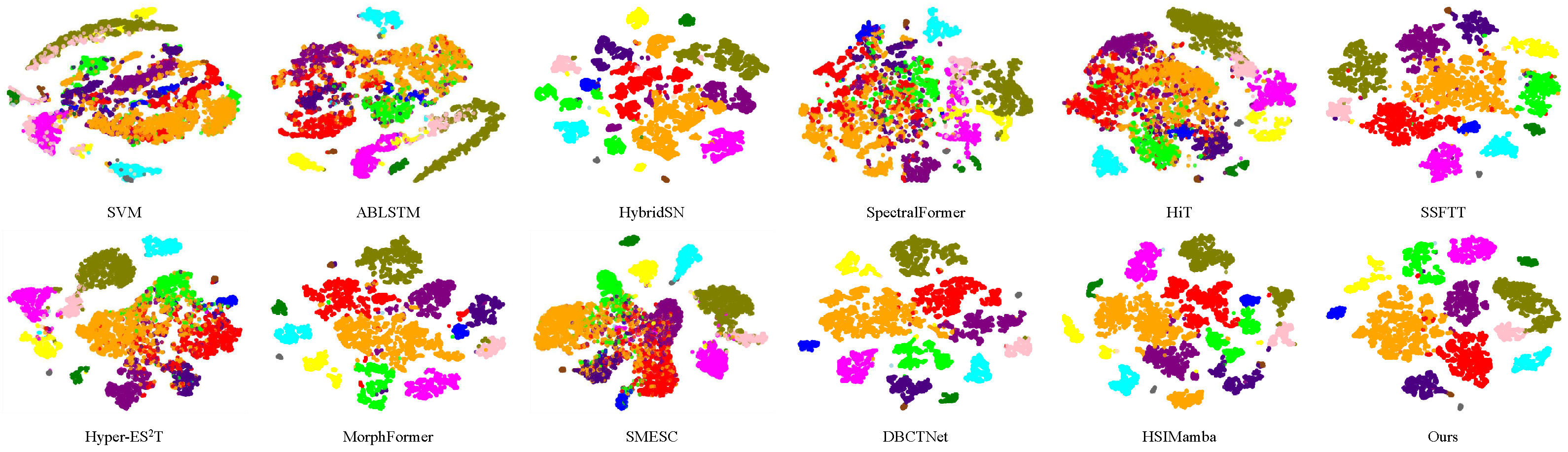
The distributions of features extracted using various methods are visualized with t-distributed stochastic neighbor embedding (t-SNE) [48], as shown in Figure 4. t-SNE, a widely used technique for dimensionality reduction, helps us understand how the model discriminates between classes in a lower-dimensional space. The visualization reveals that our model demonstrates a more cohesive separation, with greater distances between samples from different classes. In summary, the t-SNE visualization suggests that our model offers a high level of interpretability and practical effectiveness.
Additionally, quantitative classification results, encompassing OA, AA, Kappa, and per-class accuracies, are detailed in Table 4, Table 5 and Table 6 for the Indian Pines, Pavia University, and WHU-Hi-LongKou datasets. Figure 5, Figure 6 and 
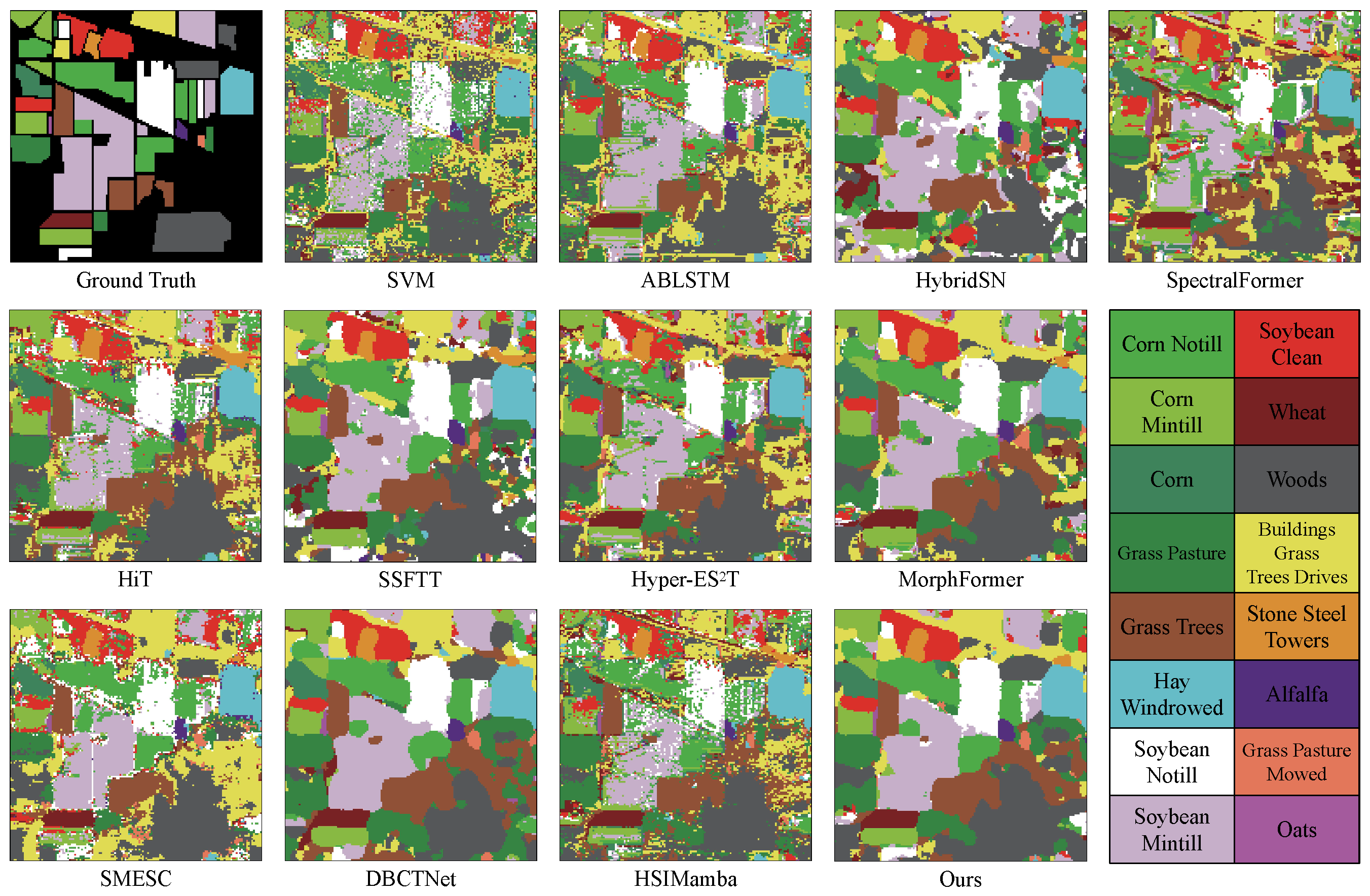
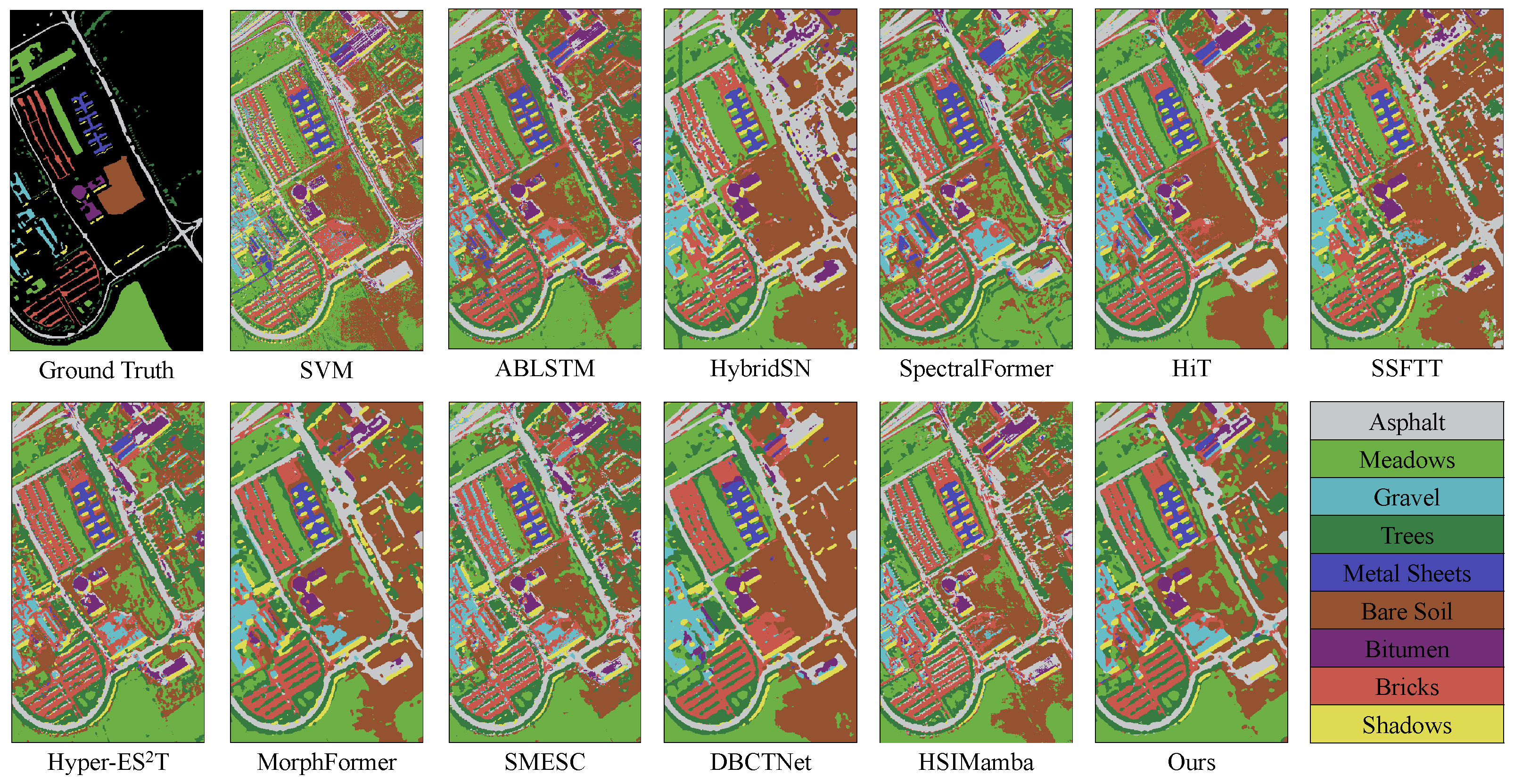
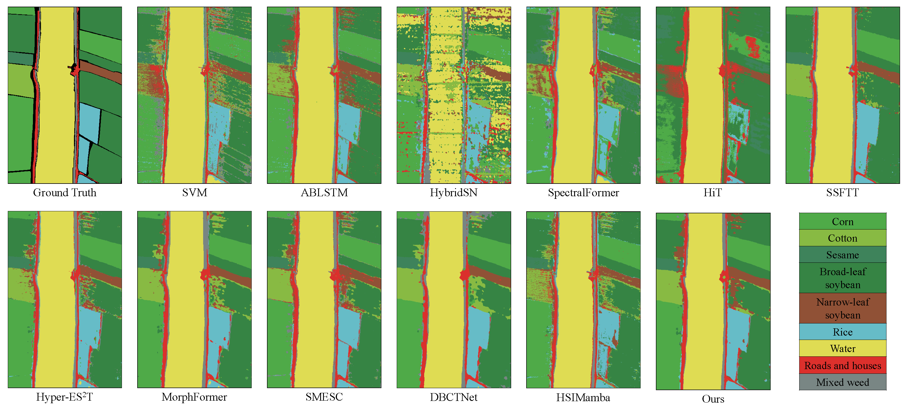
Figure 7 illustrate the qualitative results for the IP, PU, and LK datasets, respectively. Background patches are included in the visualizations for illustrative purposes, but they are excluded from both training and quantitative evaluation. For datasets like IP and PU, some background pixels are not labeled and are excluded from the reported results; for the fully annotated LK dataset, all pixels are used in training and evaluation. Background pixels do not contribute to the loss computation, ensuring that the optimization is driven solely by labeled class samples.

4.3.1. Results Based on the Indian Pines Dataset

In this section, we compare the performance of SVM, ABLSTM, HybridSN, Spectral-Former, HiT, SSFTT, Hyper-E S 2 T, MorphFormer, SMESC, DBCTNet, HSIMamba, and our proposed AMamNet on the IP dataset, as shown in Table 4.
The comparison of classification results emphasizes the superior performance of deep learning methods over traditional machine learning approaches, such as SVM. The SVM model achieved an OA of only 73.68%, significantly lagging behind deep learning models. This stark difference highlights the unique advantages of deep learning methods in effectively handling complex HSI. Among the deep learning methods evaluated, several methods, including SMESC, DBCTNet, and MorphFormer, exhibited commendable performance, with OAs of 95.62%, 95.46%, and 93.60%, respectively. However, the proposed method, AMamNet, outperformed all competitors, achieving an impressive OA of 97.62%, an AA of 98.83%, and a Kappa coefficient of 0.9727. Notably, AMamNet not only surpasses the second-best performer, DBCTNet, by 2.00% in OA but also demonstrates superior robustness, as indicated by its higher Kappa coefficient.
In details, AMamNet achieved remarkable accuracy across 15 out of 16 categories, with perfect classification in multiple instances, demonstrating its effectiveness in distinguishing even the most challenging land cover types. This excellent performance is attributed to the model’s integration of the advantages of Mamba, self-attention mechanisms, and convolutional structures, enabling it to mitigate redundant spatial and spectral features and inter-class spectral overlap.
Building on its demonstrated superiority in classification performance, AMamNet further distinguishes itself, with significant advantages in model efficiency. Specifically, AMamNet requires only 0.5 M parameters, representing a reduction of 8.7 M compared to HSIMamba, another model based on the Mamba architecture. Furthermore, our training time is 32.65 s, which is significantly faster compared to Transformer-based methods. For instance, SpectralFormer takes 62 s, and MorphFormer requires 67.05 s, while DBCTNet takes 56.89 s. Additionally, our testing time is 1.24 s, which is 2.44 s faster than SpectralFormer. This shows that our method achieves high computational efficiency, outperforming most Transformer-based architectures in both training and inference time.
The classification results of various algorithms are illustrated in Figure 5, clearly presenting the spatial distribution of different categories. The classification results of various algorithms are illustrated in 
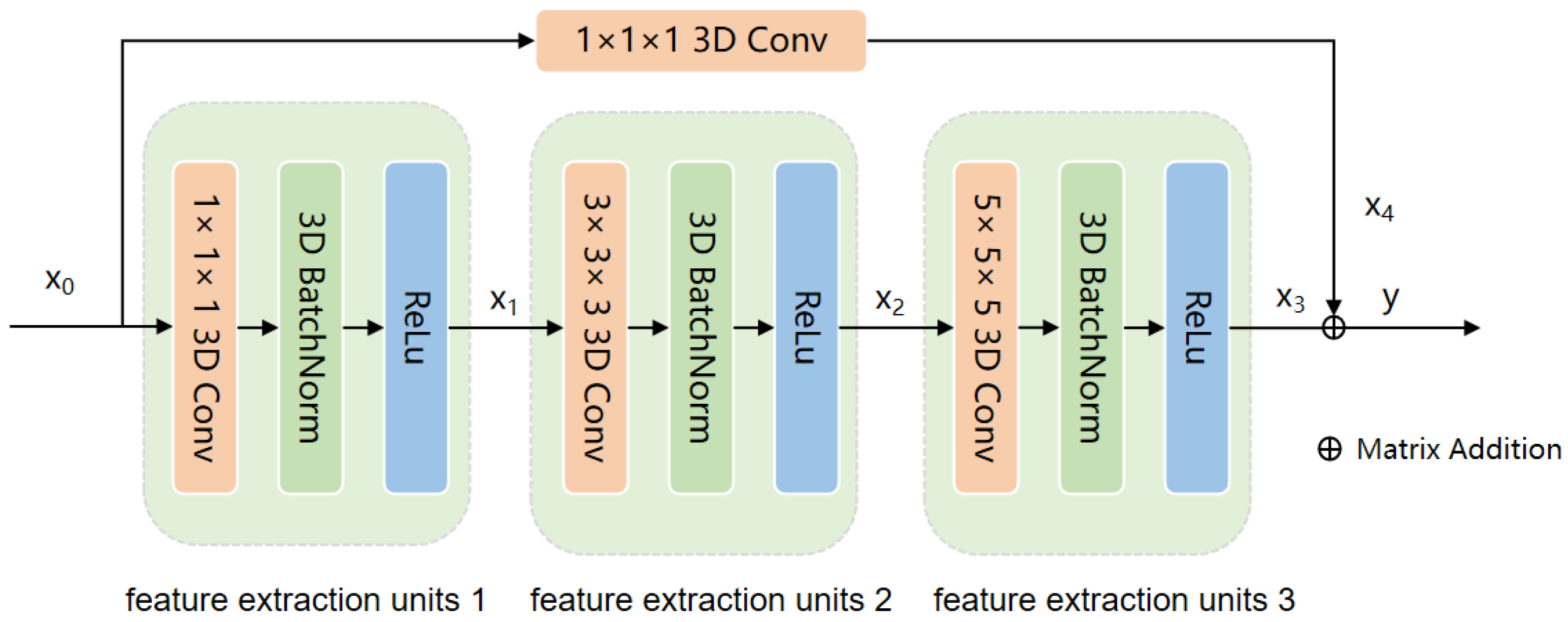
Figure 5, clearly presenting the spatial distribution of different categories. AMamNet demonstrates superior performance in challenging categories such as Soybean Mintill and Woods, with significantly reduced prediction noise compared to other models, achieving classification accuracies of 96.94% and 98.23%, respectively. This advantage is largely attributed to the 3D convolution-based Stem Conv Block module, which aggregates highly correlated spectral bands and smooths both local and global spatial features.

4.3.2. Results on Pavia University Dataset

The comparison of classification results based on the the PU dataset further confirms the superior performance of deep learning methods over traditional machine learning approaches, specifically SVM. As presented in Table 5, SVM achieved an OA of only 77.61%, significantly trailing behind the deep learning models. Figure 6 indicates that SVM tends to confuse Meadows and Bare Soil, primarily due to the similarity in reflectance values for these two categories in certain spectral bands. This similarity results in reduced classification accuracy when distinguishing between them, further highlighting the limitations of traditional machine learning methods in handling complex land cover types. In contrast, deep learning models can effectively identify these subtle differences through more advanced feature extraction mechanisms.
In the explicit comparison between deep learning methods, SMESC, DBCTNet, and MorphFormer achieved commendable OAs of 91.80%, 87.35%, and 88.89%, respectively. However, our proposed method, AMamNet, demonstrated superiority, attaining an impressive OA of 95.69%, an AA of 95.01%, and a Kappa coefficient of 0.9417, seamlessly outperforming the SSM-based method HSIMamba by a great margin. This improvement can be attributed to AMamNet’s incorporation of transformer-based dynamic tokenization, which enables the dynamic modeling of both local and global dependencies within spectral–spatial features. By leveraging this advanced mechanism, AMamNet demonstrates an enhanced capacity to capture subtle feature variations, facilitating the more accurate differentiation of complex and overlapping land cover types. Notably, AMamNet outperformed the second-best method, SMESC, by 3.89% in OA, demonstrating its superior robustness and effectiveness in HSI classification. Regarding the model’s parameters, training time and testing time, AMamNet achieves results comparable to SMESC, while demonstrating an approximately 4% improvement in the OA metric. Our training time of 141.69 s is considerably lower than HYPER-E2ST, which takes 524.25 s, and DBCTNet, the fastest Transformer-based method, by 23.22 s. In terms of testing time, our model performs well with a value of 10.01 s, which is lower than the average testing time of the compared methods, demonstrating strong efficiency in inference as well.
AMamNet, shown in Figure 6, exhibits significant separation of features among various land cover types. Compared to other competitive models, such as SMESC and DBCTNet, AMamNet exhibits more precise class boundaries and superior overall classification performance, particularly in complex categories such as Meadows and Bitumen, with recognition accuracies of 98.21% and 97.86%, respectively. This advantage stems from the incorporation of ABMB, which captures fine-grained spectral variations via a bidirectional spectral scanning mechanism. This structure effectively preserves subtle spectral differences between overlapping categories, enabling the model to maintain excellent classification performance, even in the presence of blurred class boundaries and significant spectral confusion.

4.3.3. Results on the WHU-Hi-LongKou Dataset

Finally, Table 6 displays the classification results of AMamNet in comparison to ten other algorithms on the WH-LK dataset. In this dataset, AMamNet outperforms all competitors across the three evaluation metrics, achieving an OA of 95.24%, which is 1.72% higher than that of the second-best method, DBCTNet. Specifically, in tackling challenging categories, some models, such as HybridSN, attain only 36.79% accuracy in category 4, while AMamNet excels, with an accuracy of 87.35%, the highest among all models. Furthermore, our method significantly outperforms HSIMamba, achieving an OA of 95.24%—a 4.25% improvement. This suggests that AMamNet, utilizing the ABMB and Stem Conv Block, excels at handling the complexities inherent in HSI data.
In terms of model complexity, AMamNet demonstrates a notable advantage. As shown in Table 6, the parameter size of AMamNet is 0.8M, which is smaller than that of SMESC (1.0M) and other competing methods such as Hyper-ES2T (23.1M) and HiT (64.8M). Despite its compact architecture, AMamNet achieves superior performance, highlighting the efficiency of its design. Additionally, AMamNet achieves competitive training time and testing time. In the LK dataset, due to the higher spectral dimensions, our training time of 135.8 s is slightly longer than DBCTNet’s 80.65 s, but still faster than SpectralFormer’s 111.53 s. When it comes to testing time, our method again excels, with a testing time of 24.42 s, which is much faster than HiT, which takes 65.70 s, further emphasizing our model’s superior testing speed.
AMamNet, illustrated in 
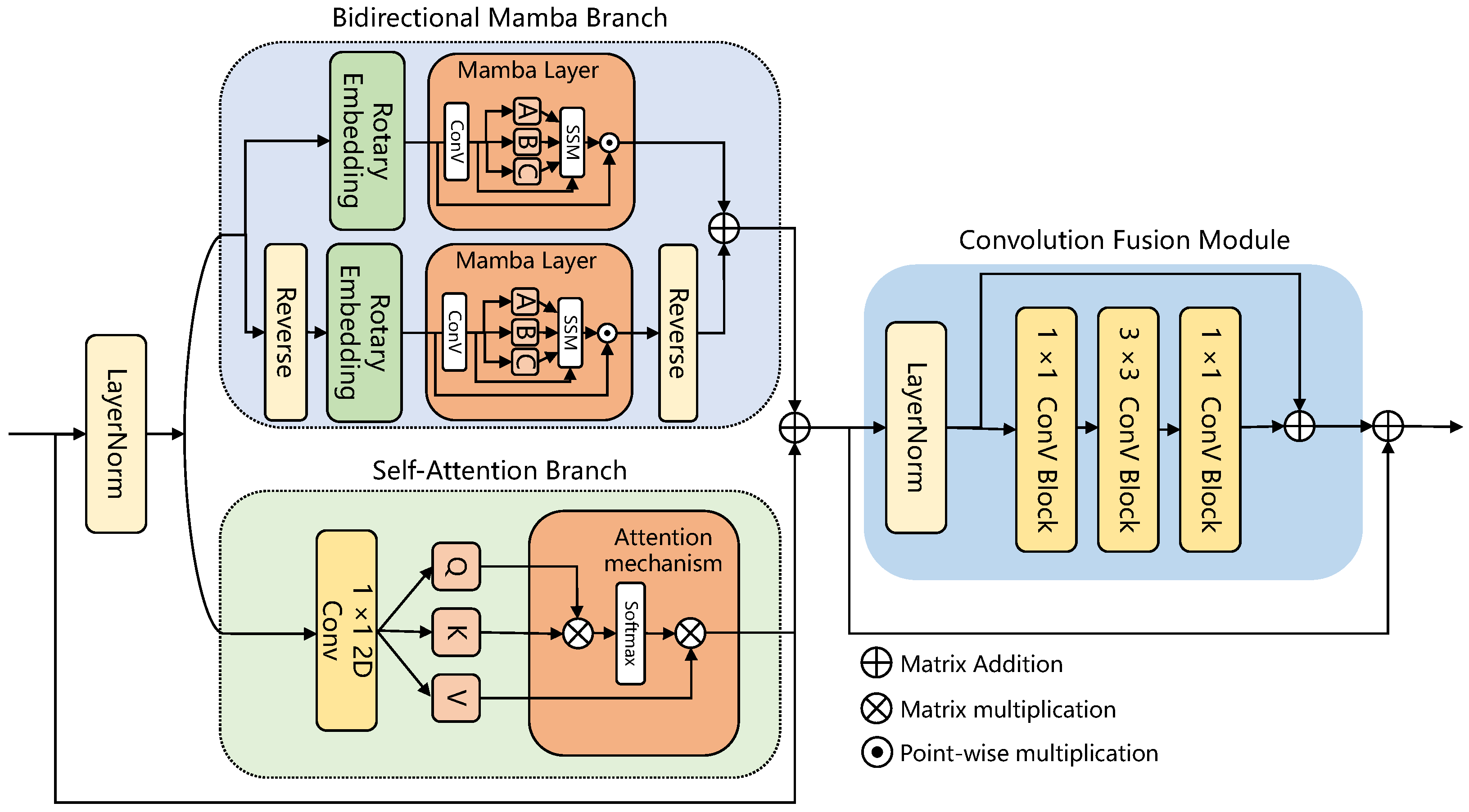
Figure 7, exhibits well-defined regions and clear boundaries, demonstrating its effectiveness in classification. For example, in categories that are generally challenging to identify, such as Broad-leaf soybean and Mixed weed, AMam-Net improved by 3.02% and 7.09%, respectively, compared to DBCTNet. From a visual perspective, AMamNet demonstrates clearer region boundaries with fewer classification noise. This significant improvement is primarily due to the integrated ABMB module. The module consists of two branches that work synergistically, leveraging their complementary strengths to model complex spectral relationships. The Self-Attention Branch introduces a context-aware attention mechanism, effectively capturing global spectral dependencies, enhancing key spectral features while suppressing irrelevant information. The Bidirectional Mamba Branch, based on the SSM, dynamically models the spectral sequence, deeply exploring and integrating trends within continuous spectral variations. The synergistic effect of these two branches enables the model to capture both local spectral relationships and long-range dependencies, effectively alleviating spectral indistinguishability and significantly improving classification accuracy for samples with high spectral similarity.

4.4. Ablation Study

In this section, we present an ablation study of our proposed AMamNet, focusing on model architecture design, followed by a robustness analysis of its performance. To ensure clarity and fairness in our results, all experiments are conducted on the Pavia University dataset under fixed implementation settings, allowing us to isolate the contributions of various architectural components.

4.4.1. Ablation Study on Attention-Bidirectional Mamba Block Design

Based on the results presented in Table 7, an ablation study was conducted to evaluate the impact of various components of the ABMB structure on the performance of the model on the PU benchmark. The analysis reveals that each component of the Mamba Branch, Self-Attention Branch, and Conv Fusion Module contributes to the overall effectiveness of AMamNet. As shown in Table 7, the best performance is achieved by the proposed AMamNet, with an OA of 95.69%, an AA of 95.01%, and a Kappa coefficient of 0.9417.
First, by retaining the Conv Fusion Module, we evaluate the impact of each individual branch. When using only the Mamba Branch, the model achieves an OA of 94.24%, an AA of 93.86%, and a Kappa coefficient of 0.9215. Although this reflects the effectiveness of bidirectional spectral modeling, the performance remains suboptimal, indicating that relying solely on spectral features is insufficient to resolve the issue of spectral confusion—especially in scenarios where different classes exhibit highly similar spectral signatures. In such cases, incorporating spatial context becomes essential to differentiate regions that are spectrally similar but spatially distinct. Conversely, when using only the Self-Attention Branch, the model achieves an OA of 94.07%, an AA of 93.48%, and a Kappa of 0.9188. This demonstrates the importance of capturing long-range spatial dependencies, which enables the model to disambiguate spatially separated regions with overlapping spectral responses. However, the slightly lower performance compared to the Mamba-only setting also suggests that spectral feature extraction alone cannot be neglected. The Mamba Branch provides fine-grained spectral representation, while the Self-Attention Branch supplies crucial spatial context. Their integration within a dual-branch architecture significantly improves the model’s ability to handle spectral similarity and enhances classification accuracy for categories that are otherwise difficult to distinguish using spectral or spatial features alone.
Next, we evaluate the significance of the Conv Fusion Module in the overall performance of the model. Specifically, when the Conv Fusion Module is removed, the OA of the model drops to 94.69%, representing a decrease of 1.00% compared to 95.69% when the module is included. The AA also declines to 94.00%, a reduction of 1.01%, while the Kappa coefficient falls to 0.9280, a decrease of 0.0137. These results indicate that the Conv Fusion Module is essential for integrating features from both the Mamba and Self-Attention Branches. It enhances spatial feature representation while effectively combining spectral information from both branches, thus improving the model’s capacity to handle complex hyperspectral data.

4.4.2. Ablation Study on Stem Conv Block Design

Next, we validate that the stem block is essential for enabling the initial fusion of spatial and spectral information in a low-dimensional space through ablation experiments. The ablation study evaluates several convolution types, including standard 2D convolution, depthwise separable (DS) convolution, and the proposed 3D convolution. As shown in Table 8, the results demonstrate that the best performance is achieved with the 3D convolution type, resulting in an OA of 95.69%, an AA of 95.01%, and a Kappa coefficient of 0.9417.
Notably, the absence of the stem convolution block results in a considerable decline in performance, as evidenced by an OA of only 80.79%, an AA of 79.22%, and a Kappa coefficient of 0.7410. This highlights the importance of early spatial–spectral feature fusion. The Stem Conv Block, through multi-scale 3D convolutions, effectively captures both spatial structures and spectral variations, reduces redundant information, and facilitates faster convergence by providing high-quality shallow features to the subsequent layers.
To assess the impact of different convolution types on this fusion, we compare standard 2D convolution, DS convolution, and 3D convolution. The results reveal that while 2D convolution focuses on spatial features, it does not adequately facilitate the interaction among spectral features, leading to an OA of 90.73%. DS convolution shows an improvement with an OA of 93.12%, but it still falls short of optimal performance due to its inability to effectively integrate features. Conversely, the 3D convolution type establishes a robust correspondence between spatial and spectral features within the convolution kernel, achieving the highest OA of 95.69%, along with an AA of 95.01% and a Kappa coefficient of 0.9417. This demonstrates that 3D convolution excels in capturing the intricate relationships between spatial and spectral features, thereby significantly improving the model’s ability to analyze complex hyperspectral data.

4.4.3. Ablation Study on Model Scale

Lastly, the impact of the scale design of our proposed ABMB is investigated. The corresponding results are displayed in Table 9, where AMamNet achieves the highest performance with an OA of 95.69%, an AA of 95.01%, and a Kappa coefficient of 0.9417 when the number of stacked modules is set to one.
As the number of stacked modules increases, a gradual decline in performance is observed. This trend can be attributed to the increased capacity of deeper architectures, which, combined with a limited number of training samples, may result in overfitting. Despite this potential for overfitting, the model continues to produce strong results even with additional stacking, highlighting the robustness of our design approach.

4.4.4. Hyperparameter Analysis

As shown in Figure 8, the learning rate of 0.0005 was chosen after extensive empirical tuning across multiple preliminary experiments. At this value, we achieved the best performance in the IP dataset, with an OA of 97.62%, AA of 98.83%, and a Kappa coefficient of 97.27%. In comparison, a learning rate of 1 × 10 4 resulted in lower performance (OA: 90.76%, AA: 91.99%, Kappa: 89.43%), while higher learning rates (0.001 and 0.005) led to decreased performance. These results demonstrate that 0.0005 provides the optimal balance between stability and classification accuracy.

4.4.5. Robustness Analysis

Given that remote sensing hyperspectral imaging often faces limited samples with human annotations, achieving effective perception under small sample conditions is imperative. Furthermore, the number of training samples is significantly smaller than the number of evaluation samples. This disparity can introduce randomness in the selection of training samples, resulting in substantial bias and leading to poor robustness.
To validate our model’s robustness, we conducted experiments on the WH-LK benchmark. We randomly sampled five different data distributions and repeated the experiments five times for each distribution, calculating the mean as the model’s prediction result. The detailed experimental results are presented in Table 10.
In the results, the model achieved an OA of 95.00%, an AA of 95.62%, and a Kappa coefficient of 0.9386 across all experiments. Notably, even with varying data distributions, the scores consistently remained high, demonstrating the model’s reliability. Furthermore, the variance for OA (0.25), AA (0.27), and Kappa (0.0037) remained relatively low, further confirming the robustness of our proposed approach in handling the challenges posed by limited training samples.

4.4.6. Training Samples’ Influence

To evaluate the robustness of our proposed method under varying amounts of training data, we conducted experiments on the WH-LK benchmark with different data ratios. As described in Table 3, the current pre-divided dataset contains approximately 50 training samples per class. Therefore, we further conducted experiments by randomly selecting 10% and 50% of the training samples from the existing partitioned dataset for additional training, while benchmarking against SMESC and DBCTNet as comparative methods. As shown in Table 11, the performance of our method consistently surpasses the other two approaches across all data ratios. It is evident that SMESC exhibits significantly weaker performance with only 10% of the training samples, achieving an OA of 54.76%, an AA of 40.56%, and a Kappa coefficient of 0.4317. This sharp decline in performance can be attributed to SMESC’s reliance on a larger number of training samples to effectively learn feature representations. In contrast, even with only 10% of the training samples, AMamNet achieves an OA of 89.64%, an AA of 81.54%, and a Kappa coefficient of 0.8662, demonstrating superior robustness and effectiveness under low-sample conditions. These results highlight the robustness and generalization capability of our method, particularly in scenarios with limited training samples, further underscoring its practical applicability in real-world cases where labeled data is scarce.

5. Conclusions and Limitation

To address the challenges of spatial–spectral redundancy and spectral confusion in HSI classification, we propose a novel method, AMamNet, which incorporates a Stem Conv Block and an Attention-Bidirectional Mamba Block. Specifically, the Stem Conv Block is designed to extract shallow features from the original HSI data, effectively reducing spectral redundancy by emphasizing relevant spectral bands and minimizing the impact of redundant information. The ABMB efficiently manages complex spectral feature extraction through its dual-branch structure, which mitigates spectral similarity by enabling the model to distinguish between similar spectral features. The Self-Attention Branch captures dependencies among spectral vectors and the Bidirectional Mamba Branch models spectral features along the token sequence. The experiments validate the superior performance of our network in addressing complex HSI classification tasks. Notably, AMamNet achieves SOTA performance on the Indian Pines, Pavia University, and WHU-Hi-LongKou datasets, demonstrating the effectiveness and robustness of our model.
Although this work significantly contributes to HSI classification through the AMamNet framework, there still remain some limitations to explore in the future. Despite achieving SOTA results on three benchmark datasets, our method still retains a relatively large number of parameters, training time and testing time. Notably, the majority of the parameters are contained within the convolution kernels. This presents several potential directions for future research. For example, further exploration could be conducted on the design of SSM for spectral feature extraction, such as employing a scanning approach that simultaneously considers both spectral and spatial dimensions, potentially reducing the need for extensive feature fusion through convolution in the model. Alternatively, deeper investigations into the integration of the attention mechanism with SSM could be pursued, such as incorporating attention-based selective designs for obtaining discrete parameters. This could help SSM identify more relevant information regarding spectral feature distribution.

Author Contributions

Conceptualization, C.L., F.W., L.L. and T.Z.; Data curation, C.L., F.W., Q.J. and T.Z.; Formal analysis, C.L., F.W., Q.J. and L.L.; Funding acquisition, C.L. and Q.J.; Investigation, C.L., F.W., Q.J. and L.L.; Methodology, C.L., F.W., L.L. and T.Z.; Project administration, C.L. and Q.J.; Resources, F.W., Q.J., L.L. and T.Z.; Software, C.L., F.W., L.L. and T.Z.; Supervision, C.L. and Q.J.; Validation, C.L., F.W., L.L. and T.Z.; Visualization, C.L. and F.W.; Writing—original draft, C.L., F.W. and Q.J.; Writing—review and editing, C.L., F.W., Q.J., L.L. and T.Z. All authors have read and agreed to the published version of the manuscript.

Funding

This work was supported by the Research and Application of Coal Inventory and Transportation Refinement Management Based on Drone Tilt Photography, E100300004 MTJY2023-06.

Institutional Review Board Statement

Not applicable.

Informed Consent Statement

Not applicable.

Data Availability Statement

The datasets presented in this article are not readily available because the data are part of an ongoing study. Requests to access the datasets should be directed to the following email address: txzhang@ustb.edu.cn.

Conflicts of Interest

Authors Chunjiang Liu and Feng Wang were employed by the company China Energy Trading Group Co., Ltd. Author Qinglei Jia was employed by the company Zhongke Tuxin (Suzhou) Technology Co., Ltd. The remaining authors declare that the research was conducted in the absence of any commercial or financial relationships that could be construed as a potential conflict of interest.

References

  1. Vali, A.; Comai, S.; Matteucci, M. Deep learning for land use and land cover classification based on hyperspectral and multispectral earth observation data: A review. Remote Sens. 2020, 12, 2495. [Google Scholar] [CrossRef]
  2. Yadav, C.S.; Pradhan, M.K.; Gangadharan, S.M.P.; Chaudhary, J.K.; Singh, J.; Khan, A.A.; Haq, M.A.; Alhussen, A.; Wechtaisong, C.; Imran, H.; et al. Multi-class pixel certainty active learning model for classification of land cover classes using hyperspectral imagery. Electronics 2022, 11, 2799. [Google Scholar] [CrossRef]
  3. Thenkabail, P.S.; Smith, R.B.; De Pauw, E. Hyperspectral vegetation indices and their relationships with agricultural crop characteristics. Remote Sens. Environ. 2000, 71, 158–182. [Google Scholar] [CrossRef]
  4. Lu, B.; Dao, P.D.; Liu, J.; He, Y.; Shang, J. Recent advances of hyperspectral imaging technology and applications in agriculture. Remote Sens. 2020, 12, 2659. [Google Scholar] [CrossRef]
  5. Sabins, F.F. Remote sensing for mineral exploration. Ore Geol. Rev. 1999, 14, 157–183. [Google Scholar] [CrossRef]
  6. Van der Meer, F.D.; Van der Werff, H.M.; Van Ruitenbeek, F.J.; Hecker, C.A.; Bakker, W.H.; Noomen, M.F.; Van Der Meijde, M.; Carranza, E.J.M.; De Smeth, J.B.; Woldai, T. Multi-and hyperspectral geologic remote sensing: A review. Int. J. Appl. Earth Obs. Geoinf. 2012, 14, 112–128. [Google Scholar] [CrossRef]
  7. Manfreda, S.; McCabe, M.F.; Miller, P.E.; Lucas, R.; Pajuelo Madrigal, V.; Mallinis, G.; Ben Dor, E.; Helman, D.; Estes, L.; Ciraolo, G.; et al. On the use of unmanned aerial systems for environmental monitoring. Remote Sens. 2018, 10, 641. [Google Scholar] [CrossRef]
  8. Li, J.; Pei, Y.; Zhao, S.; Xiao, R.; Sang, X.; Zhang, C. A review of remote sensing for environmental monitoring in China. Remote Sens. 2020, 12, 1130. [Google Scholar] [CrossRef]
  9. Melgani, F.; Bruzzone, L. Classification of hyperspectral remote sensing images with support vector machines. IEEE Trans. Geosci. Remote Sens. 2004, 42, 1778–1790. [Google Scholar] [CrossRef]
  10. Ham, J.; Chen, Y.; Crawford, M.M.; Ghosh, J. Investigation of the random forest framework for classification of hyperspectral data. IEEE Trans. Geosci. Remote Sens. 2005, 43, 492–501. [Google Scholar] [CrossRef]
  11. Hall, M.A. Correlation-Based Feature Selection for Machine Learning. Ph.D. Thesis, The University of Waikato, Hamilton, New Zealand, 1999. [Google Scholar]
  12. Erpek, T.; O’Shea, T.J.; Sagduyu, Y.E.; Shi, Y.; Clancy, T.C. Deep learning for wireless communications. Develop. Anal. Deep Learn. Archit. 2020, 27, 223–266. [Google Scholar]
  13. Li, J.; Wang, H.; Zhang, X.; Wang, J.; Zhang, T.; Zhuang, P. DVR: Towards Accurate Hyperspectral Image Classifier via Discrete Vector Representation. Remote Sens. 2025, 17, 351. [Google Scholar] [CrossRef]
  14. Wang, J.; Ma, Y.; Zhang, L.; Gao, R.X.; Wu, D. Deep learning for smart manufacturing: Methods and applications. J. Manuf. Syst. 2018, 48, 144–156. [Google Scholar] [CrossRef]
  15. Avci, O.; Abdeljaber, O.; Kiranyaz, S.; Hussein, M.; Gabbouj, M.; Inman, D.J. A review of vibration-based damage detection in civil structures: From traditional methods to Machine Learning and Deep Learning applications. Mech. Syst. Signal Process. 2021, 147, 107077. [Google Scholar] [CrossRef]
  16. Ching, T.; Himmelstein, D.S.; Beaulieu-Jones, B.K.; Kalinin, A.A.; Do, B.T.; Way, G.P.; Ferrero, E.; Agapow, P.M.; Zietz, M.; Hoffman, M.M.; et al. Opportunities and obstacles for deep learning in biology and medicine. J. R. Soc. Interface 2018, 15, 20170387. [Google Scholar] [CrossRef]
  17. Mou, L.; Ghamisi, P.; Zhu, X.X. Deep recurrent neural networks for hyperspectral image classification. IEEE Trans. Geosci. Remote Sens. 2017, 55, 3639–3655. [Google Scholar] [CrossRef]
  18. Mei, S.; Li, X.; Liu, X.; Cai, H.; Du, Q. Hyperspectral image classification using attention-based bidirectional long short-term memory network. IEEE Trans. Geosci. Remote Sens. 2021, 60, 1–12. [Google Scholar] [CrossRef]
  19. LeCun, Y.; Bottou, L.; Bengio, Y.; Haffner, P. Gradient-based learning applied to document recognition. Proc. IEEE 1998, 86, 2278–2324. [Google Scholar] [CrossRef]
  20. Krizhevsky, A.; Sutskever, I.; Hinton, G.E. Imagenet classification with deep convolutional neural networks. Adv. Neural Inf. Process. Syst. 2012, 25, 1097–1105. [Google Scholar] [CrossRef]
  21. Ahmad, M.; Shabbir, S.; Roy, S.K.; Hong, D.; Wu, X.; Yao, J.; Khan, A.M.; Mazzara, M.; Distefano, S.; Chanussot, J. Hyperspectral image classification—Traditional to deep models: A survey for future prospects. IEEE J. Sel. Top. Appl. Earth Obs. Remote Sens. 2021, 15, 968–999. [Google Scholar] [CrossRef]
  22. Bhatti, U.A.; Yu, Z.; Chanussot, J.; Zeeshan, Z.; Yuan, L.; Luo, W.; Nawaz, S.A.; Bhatti, M.A.; Ain, Q.U.; Mehmood, A. Local similarity-based spatial–spectral fusion hyperspectral image classification with deep CNN and Gabor filtering. IEEE Trans. Geosci. Remote Sens. 2021, 60, 1–15. [Google Scholar] [CrossRef]
  23. Dosovitskiy, A.; Beyer, L.; Kolesnikov, A.; Weissenborn, D.; Zhai, X.; Unterthiner, T.; Dehghani, M.; Minderer, M.; Heigold, G.; Gelly, S.; et al. An image is worth 16x16 words: Transformers for image recognition at scale. arXiv 2020, arXiv:2010.11929. [Google Scholar]
  24. You, H.; Xiong, Y.; Dai, X.; Wu, B.; Zhang, P.; Fan, H.; Vajda, P.; Lin, Y.C. Castling-vit: Compressing self-attention via switching towards linear-angular attention at vision transformer inference. In Proceedings of the IEEE/CVF Conference on Computer Vision and Pattern Recognition, Vancouver, BC, Canada, 18–22 June 2023; pp. 14431–14442. [Google Scholar]
  25. Kalman, R.E. A new approach to linear filtering and prediction problems. Trans. ASME–J. Basic Eng. 1960, 82, 35–45. [Google Scholar] [CrossRef]
  26. Gu, A.; Dao, T.; Ermon, S.; Rudra, A.; Ré, C. Hippo: Recurrent memory with optimal polynomial projections. Adv. Neural Inf. Process. Syst. 2020, 33, 1474–1487. [Google Scholar]
  27. Zhuang, P.; Zhang, X.; Wang, H.; Zhang, T.; Liu, L.; Li, J. FAHM: Frequency-Aware Hierarchical Mamba for Hyperspectral Image Classification. IEEE J. Sel. Top. Appl. Earth Obs. Remote Sens. 2025, 18, 6299–6313. [Google Scholar] [CrossRef]
  28. Xu, R.; Dong, X.M.; Li, W.; Peng, J.; Sun, W.; Xu, Y. DBCTNet: Double branch convolution-transformer network for hyperspectral image classification. IEEE Trans. Geosci. Remote Sens. 2024, 62, 5509915. [Google Scholar] [CrossRef]
  29. Yang, J.X.; Zhou, J.; Wang, J.; Tian, H.; Liew, A.W.C. Hsimamba: Hyperpsectral imaging efficient feature learning with bidirectional state space for classification. arXiv 2024, arXiv:2404.00272. [Google Scholar]
  30. Su, J.; Ahmed, M.; Lu, Y.; Pan, S.; Bo, W.; Liu, Y. Roformer: Enhanced transformer with rotary position embedding. Neurocomputing 2024, 568, 127063. [Google Scholar] [CrossRef]
  31. Yu, S.; Jia, S.; Xu, C. Convolutional neural networks for hyperspectral image classification. Neurocomputing 2017, 219, 88–98. [Google Scholar] [CrossRef]
  32. Hu, W.; Huang, Y.; Wei, L.; Zhang, F.; Li, H. Deep convolutional neural networks for hyperspectral image classification. J. Sensors 2015, 2015, 258619. [Google Scholar] [CrossRef]
  33. Chen, Y.; Jiang, H.; Li, C.; Jia, X.; Ghamisi, P. Deep feature extraction and classification of hyperspectral images based on convolutional neural networks. IEEE Trans. Geosci. Remote Sens. 2016, 54, 6232–6251. [Google Scholar] [CrossRef]
  34. Zhang, M.; Li, W.; Du, Q. Diverse region-based CNN for hyperspectral image classification. IEEE Trans. Image Process. 2018, 27, 2623–2634. [Google Scholar] [CrossRef] [PubMed]
  35. Roy, S.K.; Krishna, G.; Dubey, S.R.; Chaudhuri, B.B. HybridSN: Exploring 3-D–2-D CNN feature hierarchy for hyperspectral image classification. IEEE Geosci. Remote Sens. Lett. 2019, 17, 277–281. [Google Scholar] [CrossRef]
  36. Roy, S.K.; Deria, A.; Shah, C.; Haut, J.M.; Du, Q.; Plaza, A. Spectral–spatial morphological attention transformer for hyperspectral image classification. IEEE Trans. Geosci. Remote Sens. 2023, 61, 1–15. [Google Scholar] [CrossRef]
  37. Sun, H.; Zheng, X.; Lu, X.; Wu, S. Spectral–spatial attention network for hyperspectral image classification. IEEE Trans. Geosci. Remote Sens. 2019, 58, 3232–3245. [Google Scholar] [CrossRef]
  38. Hong, D.; Han, Z.; Yao, J.; Gao, L.; Zhang, B.; Plaza, A.; Chanussot, J. SpectralFormer: Rethinking hyperspectral image classification with transformers. IEEE Trans. Geosci. Remote Sens. 2021, 60, 5518615. [Google Scholar] [CrossRef]
  39. Yang, X.; Cao, W.; Lu, Y.; Zhou, Y. Hyperspectral image transformer classification networks. IEEE Trans. Geosci. Remote Sens. 2022, 60, 5528715. [Google Scholar] [CrossRef]
  40. Wang, W.; Liu, L.; Zhang, T.; Shen, J.; Wang, J.; Li, J. Hyper-ES2T: Efficient spatial–spectral transformer for the classification of hyperspectral remote sensing images. Int. J. Appl. Earth Obs. Geoinf. 2022, 113, 103005. [Google Scholar] [CrossRef]
  41. Yu, C.; Zhu, Y.; Song, M.; Wang, Y.; Zhang, Q. Unseen feature extraction: Spatial mapping expansion with spectral compression network for hyperspectral image classification. IEEE Trans. Geosci. Remote Sens. 2024, 62, 5521915. [Google Scholar] [CrossRef]
  42. Gu, A.; Goel, K.; Ré, C. Efficiently modeling long sequences with structured state spaces. arXiv 2021, arXiv:2111.00396. [Google Scholar]
  43. Gu, A.; Dao, T. Mamba: Linear-time sequence modeling with selective state spaces. arXiv 2023, arXiv:2312.00752. [Google Scholar]
  44. Wang, G.; Zhang, X.; Peng, Z.; Zhang, T.; Jiao, L. S2Mamba: A Spatial-spectral State Space Model for Hyperspectral Image Classification. arXiv 2024, arXiv:2404.18213. [Google Scholar] [CrossRef]
  45. Ahmad, M.; Butt, M.H.F.; Usama, M.; Altuwaijri, H.A.; Mazzara, M.; Distefano, S. Multi-head Spatial-Spectral Mamba for Hyperspectral Image Classification. arXiv 2024, arXiv:2408.01224. [Google Scholar] [CrossRef]
  46. Xu, R.; Yang, S.; Wang, Y.; Du, B.; Chen, H. A survey on vision mamba: Models, applications and challenges. arXiv 2024, arXiv:2404.18861. [Google Scholar]
  47. Sun, L.; Zhao, G.; Zheng, Y.; Wu, Z. Spectral-Spatial Feature Tokenization Transformer for Hyperspectral Image Classification. IEEE Trans. Geosci. Remote Sens. 2022, 60, 5522214. [Google Scholar] [CrossRef]
  48. Van der Maaten, L.; Hinton, G. Visualizing data using t-SNE. J. Mach. Learn. Res. 2008, 9, 2579–2605. [Google Scholar]
Figure 1. Architecture illustration of our proposed AMamNet. Our method is composed of the Stem Conv Block, the Attention-Bidirectional Mamba Block, and a classifier. N represents the stack number of Attention-Bidirectional Mamba Block.
Atmosphere 16 00541 g001
Figure 2. Architecture illustration of the Stem ConV Block.
Atmosphere 16 00541 g002
Figure 3. Architecture illustration of the Attention Bidirectional Mamba Block. The Bidirectional Mamba Branch and the Self-Attention Branch complement each other in spectral modeling, while the Convolution Fusion Module enables the effective fusion of spectral and spatial features.
Atmosphere 16 00541 g003
Figure 4. Feature distribution (t-SNE [48] visualization) obtained by different methods for the IP dataset.
Atmosphere 16 00541 g004
Figure 5. The classification maps obtained by different models on the Indian Pines dataset. Note that the black regions in the Ground Truth represent unlabeled areas.
Atmosphere 16 00541 g005
Figure 6. Classification maps obtained by different models on the Pavia University dataset. Note that the black regions in the Ground Truth segment represent unlabeled areas.
Atmosphere 16 00541 g006
Figure 7. Classification maps obtained by different models on the WHU-Hi-LongKou dataset. Note that the black regions in the Ground Truth segment represent unlabeled areas.
Atmosphere 16 00541 g007
Figure 8. Classification results of the learning rate on the IP dataset.
Atmosphere 16 00541 g008
Table 1. Categories of the information from the IP dataset.
Category No.Category NameTrainingEvaluation
1Corn Notill501384
2Corn Mintill50784
3Corn50184
4Grass Pasture50447
5Grass Trees50697
6Hay Windrowed50439
7Soybean Notill50918
8Soybean Mintill502418
9Soybean Clean50564
10Wheat50162
11Woods501244
12Buildings Grass Trees Drives50330
13Stone Steel Towers5045
14Alfalfa1539
15Grass Pasture Mowed1511
16Oats155
Total6959671
Table 2. Categories of the information from the PU dataset.
Category No.Category NameTrainingEvaluation
1Asphalt5486304
2Meadows54018,146
3Gravel3921815
4Trees5242912
5Metal Sheets2651113
6Bare Soil5324572
7Bitumen375981
8Bricks5143364
9Shadows231795
Total392140,002
Table 3. Categories of the information from the WH-LK dataset.
Category No.Category NameTrainingEvaluation
1Corn5434,457
2Cotton538321
3Sesame542977
4Broad-leaf soybean5363,159
5Narrow-leaf soybean544097
6Rice5011,804
7Water5367,003
8Roads and houses537071
9Mixed weed515178
Total475204,067
Table 4. Comparison of quantitative results based on the IP dataset. The best performance is shown in bold.
Category No.SVMABLSTMHybridSNSpectralFormerHiTSSFTTHyper-ES2TMorphFormerSMESCDBCTNetHSIMambaOurs
167.2769.8789.3156.2167.4983.9670.5990.5383.5391.1184.5094.22
264.9285.3393.7582.7884.8294.9084.0697.7093.4999.2380.18100.00
385.8788.0494.5792.3992.9397.8395.11100.0099.46100.0098.86100.00
493.2994.8595.9789.4993.9695.3096.6498.6695.5394.6396.9198.43
585.9486.8098.4262.5596.8499.8692.9796.1399.43100.0096.70100.00
695.4496.8199.7792.9497.2799.5498.1899.77100.00100.0099.94100.00
775.0582.6888.0271.1376.8091.2983.5589.2275.0588.4580.7397.17
858.0676.3983.5457.2869.9876.8872.3789.4559.1496.2870.1796.94
978.7278.0194.3373.4073.5889.7274.2992.2055.3292.0265.0796.28
1098.7798.77100.00100.00100.00100.00100.00100.00100.00100.00100.00100.00
1187.5492.2895.2679.5092.6895.6696.0697.1995.4297.5995.8098.23
1265.7687.8895.7687.8898.7998.7990.0099.0997.58100.0099.39100.00
1395.5697.78100.00100.00100.00100.00100.00100.00100.00100.00100.00100.00
1482.0592.3197.4482.0589.74100.0089.74100.0092.31100.0095.55100.00
1590.91100.00100.00100.00100.00100.00100.00100.00100.00100.00100.00100.00
16100.00100.00100.00100.00100.00100.00100.00100.00100.00100.00100.00100.00
OA(%)73.6882.6491.2070.5981.0889.1982.8093.6080.9695.6289.2397.62
AA(%)82.8289.2495.3882.9889.6895.2390.2296.8790.3997.4691.4998.83
Kappa0.70270.80220.89950.66920.78550.87720.80440.92680.78430.94960.88360.9727
Params-1.6M0.4M1.0M59.3M0.2M12.7M0.3M0.6M0.03M9.2M0.5M
Training Time0.19 s21.52 s9.76 s62.00 s134.52 s21.96 s95.20 s67.05 s30.93 s56.89 s539.74 s32.65 s
Te sting Time0.58 s0.86 s0.53 s3.68 s6.03 s0.68 s3.12 s2.72 s1.42 s1.05 s53.86 s1.24 s
Table 5. Comparison of quantitative results based on the PU dataset. The best performance is shown in bold.
Category No.SVMABLSTMHybridSNSpectralFormerHiTSSFTTHyper-ES2TMorphFormerSMESCDBCTNetHSIMambaOurs
175.0284.3193.5177.0181.2787.2887.4888.3178.8792.1577.2793.48
268.6096.3766.7381.0084.8267.6296.3684.3398.0373.4780.2398.21
372.3455.1077.1361.9873.4979.1760.7283.7569.3187.4463.2582.47
490.9399.4578.3395.9191.0790.6699.4293.7596.8474.2196.6798.52
599.1998.7499.8298.7499.28100.0099.7398.9299.2899.8299.2899.55
691.2383.9599.4856.8999.3094.7758.5993.6888.0199.1973.9987.97
788.5685.7393.7866.8782.3697.7689.4098.5785.9398.8866.5697.86
8100.0096.4395.7291.6597.0091.2996.5598.3993.9198.9694.7498.90
9100.0094.9796.7393.9692.7099.1296.9897.7494.7296.7389.8198.11
OA(%)77.6191.1880.6379.1481.0380.2889.2088.8991.8087.3581.0895.69
AA(%)85.9388.3489.0380.4587.4889.7487.2593.0589.4373.3882.4295.01
Kappa0.71570.88100.75500.72460.75850.75020.85230.85440.88940.85450.75170.9417
Params-0.5M0.4M0.4M54.5M0.2M3.7M0.2M0.1M0.01M6.0M0.2M
Training Time0.70 s93.74 s71.64 s297.95 s945.65 s73.55 s524.25 s373.68 s131.9 s164.91 s2853.09 s141.69 s
Te sting Time16.14 s6.67 s5.78 s19.78 s87.30 s4.25 s25.46 s23.04 s4.09 s7.91 s556.09 s10.01 s
Table 6. Comparison of quantitative results based on the WH-LK dataset. The best performance is shown in bold.
Category No.SVMABLSTMHybridSNSpectralFormerHiTSSFTTHyper-ES2TMorphFormerSMESCDBCTNetHSIMambaOurs
185.1694.8989.5389.8099.0397.9198.9598.3695.6099.0397.1298.18
227.7679.4479.0058.7383.2891.2192.3496.9896.2399.6978.3699.38
353.2180.8595.0670.0788.8892.2488.2186.3381.7394.1984.5190.29
469.8182.1936.7970.6379.4878.0484.0684.0179.3184.3383.6587.35
581.5796.9275.1575.1089.5095.1992.4693.1987.8995.1787.7096.78
684.2293.0079.4373.8998.6792.4396.2397.0397.5698.7985.1598.99
799.9999.8674.4799.3999.1198.9299.5699.3899.9599.5998.3499.98
883.8491.0663.1589.5588.6085.7097.0491.4790.3493.6690.1196.62
942.9375.3266.4385.6985.1178.5290.6793.4092.1488.1885.8295.27
OA(%)81.2391.0665.5484.1391.2990.4593.5593.4891.5094.0790.9995.24
AA(%)69.8388.1773.2379.2190.1990.0293.2893.3591.1994.7487.8695.87
Kappa0.76120.88470.56900.79770.88810.87720.91660.91570.89090.92330.88370.9383
Params-2.8M0.4M1.7M64.8M0.2M23.1M0.3M1.0M0.04M11.5M0.8M
Training time3.69 s31.44 s23.26 s111.53 s179.11 s25.09 s306.03 s368.43 s96.65 s80.65 s3484.07 s135.8 s
Te sting Time4.09 s12.75 s4.87 s52.95 s65.70 s5.28 s51.17 s29.48 s14.68 s15.79 s571.89 s16.85 s
Table 7. Ablation study on designs for the ABMB structure on the PU benchmark. A checkmark (✓) indicates the inclusion of a component, while a cross (×) denotes its exclusion. The best performance is shown in bold.
StructuresEvaluation Metrics
Mamba BranchSelf-Attention BranchConv Fusion ModuleOA(%)AA(%)Kappa
×94.2493.860.9215
×94.0793.480.9188
×94.6994.000.9280
95.6995.010.9417
Table 8. Ablation study on designs for the Stem block structure on the PU benchmark. DS represents depthwise separable convolution, ‘-’ represents not available, and a checkmark (✓) indicates the inclusion of a component. The best performance is shown in bold.
StructuresEvaluation Metrics
Stem BlockConvolution TypeOA(%)AA(%)Kappa
--80.7979.220.7410
2D90.7392.270.8765
DS93.1292.250.9070
3D95.6995.010.9417
Table 9. Ablation study on model scale design on the PU benchmark. The best performance is shown in bold.
Evaluation Metrics
OA(%)AA(%)Kappa
195.6995.010.9417
295.1794.940.9352
394.9694.740.9319
Table 10. Analysis of the robustness evaluation on the WH-LK benchmark.
Evaluation Metrics
OA(%)AA(%)Kappa
194.9695.350.9324
294.5295.540.9267
395.2596.070.9364
495.0995.280.9340
595.1795.510.9374
mean95.0095.620.9386
variance0.250.270.0037
Table 11. Analysis of the training samples’ influence on the WH-LK benchmark.
MethodData RatioEvaluation Metrics
OA(%)AA(%)Kappa
10%54.7640.560.4317
SMESC50%90.3689.570.8765
100%91.5091.190.8909
10%86.2864.390.8223
DBCTNet50%91.1193.790.8863
100%94.0794.740.9233
10%89.6481.540.8662
AMamNet50%92.9888.090.9088
100%95.2495.870.9383
Disclaimer/Publisher’s Note: The statements, opinions and data contained in all publications are solely those of the individual author(s) and contributor(s) and not of MDPI and/or the editor(s). MDPI and/or the editor(s) disclaim responsibility for any injury to people or property resulting from any ideas, methods, instructions or products referred to in the content.

