Analytical Approach to Enhancing Efficiency of Silt Loading Collection in EPA Vacuum Sweep Method Using K-Means Clustering

Abstract

This study explores the application of K-means clustering to optimize the selection of sampling locations for suspended silt loading (sL) on asphalt pavements, addressing the limitations of traditional random sampling methods in the EPA method. The objective was to identify reliable sampling points for road dust concentration measurement, with a focus on improving the accuracy of data collection using the vacuum sweep method. The elbow method was used to determine the optimal number of clusters, revealing that three clusters were ideal for 25 m intervals and five for 100 m intervals. The clustering analysis identified specific sampling locations within the 25 m and 100 m road sections, such as 1.5–4.5 m and 12–18 m, and 15–18 m, 39–42 m, 57 m, 69 m, and 87 m, respectively, which adequately captured sL characteristics. The silhouette score of 0.6247 confirmed the effectiveness of the clustering method in distinguishing distinct groups with similar sL characteristics. The comparison of clustered versus non-clustered sections across 15 pavement segments showed an error rate of approximately 6%. Properly selecting sampling points ensures more accurate dust concentration data, which is crucial for effective road maintenance and environmental management. The findings highlight that optimizing the sampling process can significantly enhance the precision of dust monitoring, especially in areas with varying sL characteristics.

1. Introduction

Particulate matter (PM) with a diameter smaller than 10 μm poses significant health risks, including respiratory failure and mental disorders [1]. In particular, PM has been strongly associated with elevated risks of both mortality and morbidity, particularly due to cardiovascular and respiratory diseases, as well as chronic conditions such as diabetes and pneumonia. These adverse health effects have been consistently documented in epidemiological studies across various regions, emphasizing the urgent need for effective PM control in urban environments [2,3]. The severity of these impacts increases with smaller particle sizes. PM₁₀ can penetrate the upper respiratory tract, while finer particles such as PM_2.5 reach deeper into the lungs. Ultrafine particles like PM₁ are particularly concerning as they can infiltrate the alveoli and even enter the bloodstream, potentially affecting multiple organ systems. Due to their varying penetration capabilities and persistence in the air, all forms of PM remain critical targets for air quality management and public health interventions [3,4].

PM concentrations are particularly elevated in proximity to roadways [4], necessitating effective management strategies within road maintenance frameworks. Quantitative analysis of contamination levels is essential for determining the need for mitigation measures. Road dust (RD), generated and dispersed by vehicular activity, constitutes a major source of urban pollution. It comprises both exhaust emissions (EEs), originating from internal combustion engines, and non-exhaust emissions (NEEs), which result from tire wear, brake wear, and road surface abrasion [5]. The dispersion of suspended road dust, driven by traffic and wind, is commonly assessed using silt loading (sL, units: g/m²), which quantifies the mass of dust particles (≤75 µm) per unit road surface area [4]. The conventional sL measurement method utilizes the vacuum sweep technique, which is labor-intensive, costly, and constrained by temporal and spatial limitations [6,7]. As an alternative, mobile laboratories enable real-time road dust measurement during driving, facilitating the generation of RD distribution maps and supporting dust mitigation strategies [8,9]. However, in South Korea, RD mapping is conducted bi-monthly, and the inability to repeatedly survey identical locations restricts real-time response capabilities. Furthermore, certain mobile laboratories do not incorporate simultaneous sL assessments, limiting the accuracy of national dust emission estimations. Although systematic national-level intervention has been limited, several local governments in Korea—such as those of Seoul and Incheon—have introduced regional air quality management policies. These include the designation of fugitive dust control zones, the application of stricter construction site regulations, and the use of real-time monitoring systems to better assess and manage local dust emissions [10,11]. Traditional sL measurement follows the AP-42 method to minimize errors; however, the U.S. Environmental Protection Agency (EPA) methodology, which employs random sampling along 2.4 km (1.5-mile) road segments, is challenging to implement in South Korea due to shorter average intersection distances (500 m), permitting only two sampling points per segment [6].

The limited number of sampling points due to shorter intersection spacing presents a challenge for the direct application of this methodology in South Korea [12]. To address this limitation, some studies have proposed alternative sL collection methods under varying conditions. One approach involves defining a sampling section as 0.8 km, considering the absence of pavement in certain areas, as outlined in the South Korean EPA guidelines, and the relatively short intersection distances compared to the United States [13]. Accordingly, the sampling width along the measured road segment is set between 0.3 km and 0.5 km and the length to 0.8 km to ensure a minimum sample weight of 400 g [14]. Since it is impractical to collect dust from the entire road segment, further research has been conducted to refine sampling methodologies and determine optimal sampling sections. An effective sampling strategy involved defining sampling areas of 1 × 1 m², 2 × 2 m², and 4 × 1 m² at five to six points along the sL dust accumulation zone, with sampling points spaced 10 m apart. Statistical analysis using coefficient of variation (CV) analysis showed high variability (9–75%) across the sampling areas. Consequently, further investigation is required to optimize the separation distance and sampling dimensions for sL assessment [15]. Conventional sampling methods typically collect only one sample per section, assuming an average traffic signal spacing of approximately 0.8 km (0.5 miles) or less [12]. The sampling area is first delineated by traversing the road, with a standardized width of 3 m along the roadway direction [12,13,14,15]. Given the spatial variability of sL pollution distribution, a more systematic and robust statistical approach is essential to enhance measurement uniformity. Random sampling methods, often used in traditional approaches, are insufficient for effectively covering road intersections in South Korea, as dust loads can vary significantly across different road sections. Furthermore, the reliance on random values from statistical tables presents challenges for practical implementation.

To address these issues, advanced analytical techniques such as artificial intelligence (AI) and clustering methods should be considered to optimize sL sampling locations [15]. As sL assessment becomes increasingly crucial, improving the efficiency of dust collection methodologies is vital. Clustering techniques, including K-means and hierarchical clustering, offer significant advantages by grouping road sections with similar dust concentrations. This allows for the identification of high-risk areas and spatial patterns in dust distribution, leading to more targeted and efficient sampling. These methods minimize redundancy in measurements and improve the accuracy of dust emission estimates by focusing on areas with higher pollutant concentrations, which random sampling might overlook. Additionally, integrating clustering-based analysis with mobile laboratory data enhances real-time monitoring, optimizes resource allocation, and supports more effective road dust management strategies in related countries. By applying clustering techniques, the accuracy of dust emission predictions can be substantially improved, ensuring that sampling efforts are both cost-effective and comprehensive.

2. Materials and Methods

2.1. sL Measurement Using EPA AP-42

The conventional methods for measuring road dust are primarily based on the U.S. EPA’s AP-42 guidelines. This approach originally involves sampling the entire road section, but due to practical constraints, the EPA does not permit complete road section sampling. Instead, samples are collected from randomly selected locations along a 1.5-mile (2.4 km) segment using the vacuum sweep method [6]. This method estimates sL in grams per square meter (g/m²) by measuring the weight of particles smaller than 75 μm deposited per unit area (m²). While this method provides a standardized approach, it has notable limitations in fully capturing the spatial variability of dust loads across the entire road section. The random sampling inherent in the vacuum sweep method may fail to accurately represent areas with higher dust accumulation, such as road intersections or high-traffic zones, leading to potential inaccuracies in dust emission estimates. In comparison, the broom sweep method is a simpler and less expensive alternative that involves manually collecting dust using a broom. Upright stick broom vacuums use relatively small, lightweight filter bags, while bags for industrial-type vacuums are bulky and heavy. Because the mass collected is usually several times greater than the bag tare weight, uprights are thus well suited for collecting samples from lightly loaded road surfaces. On the other hand, on heavily loaded roads, the larger industrial-type vacuum bags are easier to use and can be more readily used to aggregate incremental samples from all road surfaces.

These features are discussed further below. However, this method is also subject to several disadvantages. One significant drawback is its inherent subjectivity and inconsistency, as the effectiveness of dust collection heavily depends on the operator’s technique. Furthermore, this method is less effective at capturing fine spatial variations in dust accumulation. While it may be useful for small or localized studies, it does not offer the same level of consistency or precision as the vacuum sweep method, particularly in large-scale applications. Despite the widespread adoption of both the vacuum sweep and broom sweep methods for road dust sampling, these techniques have limitations that hinder their ability to accurately represent the full range of dust distribution, especially in urban environments where dust levels can vary significantly. The random nature of the vacuum sweep method may not provide sufficient detail for targeted dust management, while the manual and subjective nature of the broom sweep method limits its precision.

The U.S. EPA’s AP-42 methodology offers a widely accepted approach to estimating road dust emissions, particularly sL, based on surface characteristics and traffic conditions. As this method is well documented, only relevant parameters applied in this study are briefly summarized in

Table 1. EPA AP-42 Appendix C.1 procedures for sampling surface dust loading.

Method	Selection of Section	Sampling Method
Selection of sampling location	Road segment	Samples are collected at intervals of 0.8 km along the roadway, specifically between sections with different pavement types or intersections with unpaved roads.
	1 km (0.6-mile) section	Two samples are randomly selected within 1 km.
	Less than 2.4 km (1.5 miles)	For roads shorter than 2.4 km, a total of three samples are collected, as follows: (1) The first sample is taken from a randomly selected location within the initial 0.8 km, corresponding to the distance between intersections. (2) Additional sampling points are determined by generating three random numbers (x1, x2, x3) using the following method: referencing statistical tables to obtain pseudorandom numbers using an engineering calculator for random number generation. (3) Random number generation algorithms are applied to create random sequences based on user-defined input values.
	More than 2.4 km (1.5 miles)	At least three samples are collected for every 4.8 km road segment: (1) The first sample is taken from a randomly selected location within the road segment unit between intersections. (2) Two additional samples are collected within the 0.8 km to 4.8 km range, excluding the first sampling point.
	Horizontal length and width	(1) Samples are collected only from straight road sections, excluding curved segments. (2) The lateral sampling width within a single sampling interval is set to 0.3 m (1 ft) for visibly dirty roads and 3 m (10 ft) for visually clean roads. (3) Sampling is conducted within a designated range that excludes curbside sections and road markings, such as white lane markings along the centerline.

[16,17,18].

Given that road dust can be washed away by rainfall, which influences its accumulation, sampling was conducted on days with minimal precipitation, specifically on days when rainfall intensity did not exceed 0.254 mm/h, as recommended by AP-42 Section 13.2.3 for conditions impacting road dust levels [19].

Although both the vacuum sweep and broom sweep methods are widely adopted for road dust sampling, their limitations highlight the need for more systematic and advanced approaches, particularly in environments where dust distribution is highly variable. The random sampling in the vacuum sweep method does not provide sufficient detail for targeted dust management, while the manual broom sweep method lacks the precision needed for large-scale studies. Therefore, alternative approaches—such as clustering or advanced statistical analysis—could offer more reliable and efficient ways to capture the full range of spatial variability in road dust levels. These advanced methods would provide better insights for environmental management and dust emission estimates, enhancing the effectiveness of dust mitigation strategies.

2.2. Study Area

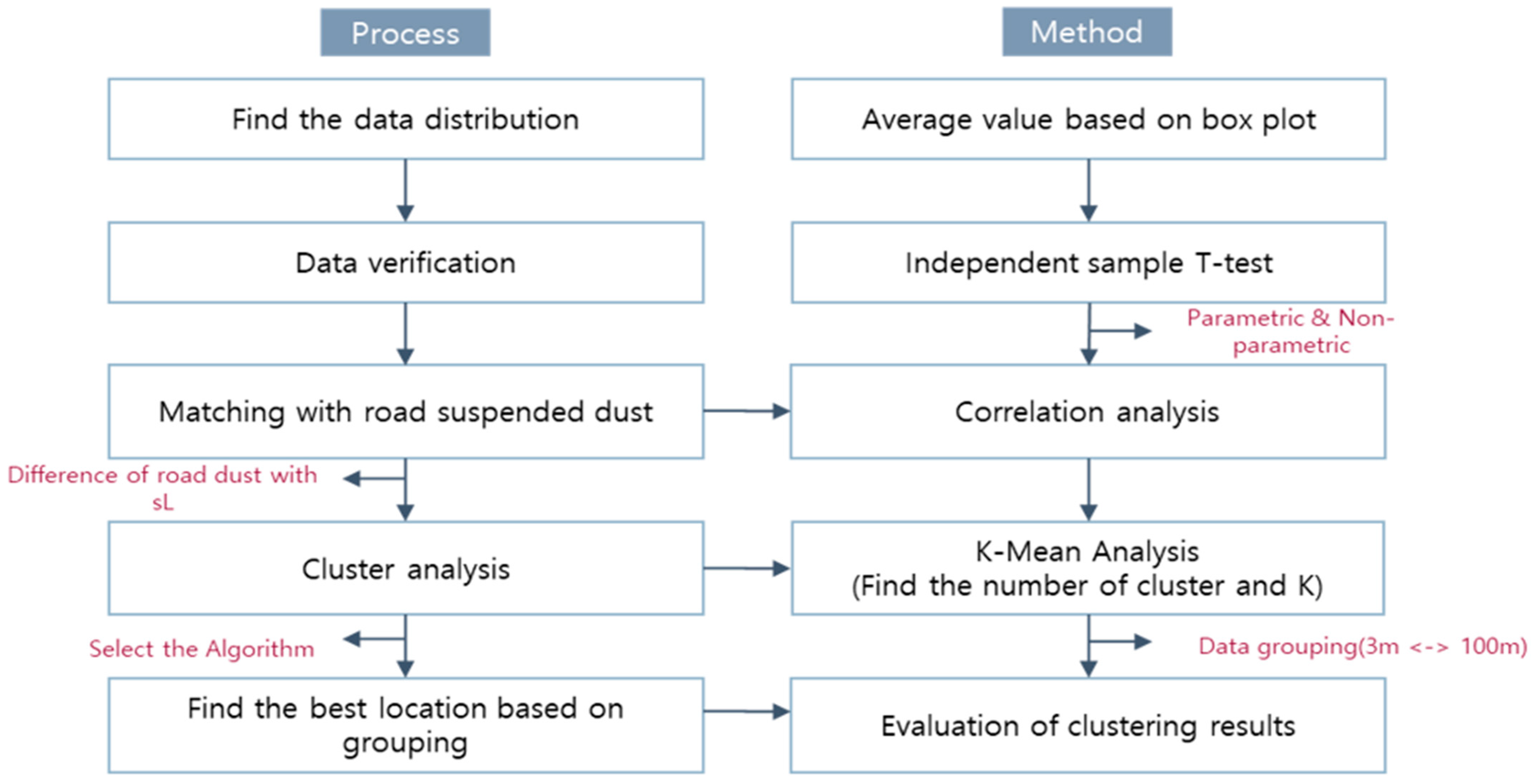
To enhance the efficiency of the vacuum sweep method for sL measurement, representative sampling locations were selected based on vehicle operating conditions and environmental factors. Given the increasing significance of sL in road dust pollution assessments, optimizing dust collection methods was a priority. Measurements were conducted across four sections from June to September 2023, during time periods of minimal traffic disruption, to ensure accurate sL evaluation. When selecting the sections, dust load sampling was performed in areas where homogeneity could be secured to minimize the effect on the background fine dust concentration. Verification sampling was conducted on a test road, which was blocked from traffic, ensuring that the dust collection process was not influenced by vehicle traffic. This allowed for a more controlled environment, where dust was collected without interference from vehicle emissions or traffic-related disturbances.

Moreover, since the amount of dust collected varies depending on the characteristics of each road section, sampling was conducted across different sections to account for this variability. By covering a wide range of road types, the potential for applying clustering techniques to optimize sampling locations was enhanced. Additionally, to improve data reliability, sampling was performed under stable weather conditions, excluding days with significant rainfall (≥0.01 inches) that could influence dust accumulation or resuspension [19]. Clustering techniques were integrated to identify optimal sampling locations, thereby enhancing efficiency, minimizing redundancy, and improving the accuracy of sL-based road dust assessments, as described in Figure 1.

2.3. Road Suspended Dust Measurement

The measurement of road suspended PM₁₀ was carried out using a resuspension monitoring system equipped with optical sensors. These sensors continuously sampled PM₁₀ every second, using two inlets: one mounted at the front of the vehicle (on the hood) and the other positioned near the right front tire, directly behind the wheel, to measure tire-induced resuspension effects [20]. This method allows for the quantification of both optical and physical characteristics of resuspended dust. Specifically, the system measures real-time dust concentrations by detecting light scattered by airborne particles, thereby estimating the mass of dust as it passes through the sensing unit [21]. A schematic of the measurement configuration is shown in Figure 2.

To summarize, the equipment contains six main components:

1. Vehicle specifications: 2016 SUV Sportage(KIA, South Korea) 2.02 WD, Tire Model 225/60R17.

2. PM₁₀ sensor: The 8530 Dust-Trak Optical PM Sensor Model (TSI Company, USA) with a PM₁₀ inlet is a portable device that can measure the concentrations of various sizes of dust particles in real time, such as PM₁₀ and PM_2.5.

3. Inlet: The right tire line inlet is 175 mm above the ground and 50 mm behind the tire. The PM₁₀ concentration (C_i) obtained from the back of the tire during movement indicates that the air velocity measured along the center of the tire is not significantly affected by the surrounding wind direction at a distance less than 100 mm from the tire [22].

4. Uniform velocity flow sampling inhalation: A vacuum pump is controlled by a customized suction port to adjust the pressure of the suction port appropriately, thereby producing a pressure-free suction port, so the air flow that is being sampled has the same fluid flow as the surrounding air flow.

5. Data collection system: Laptop computers are used to collect and transmit Dust-Trak data at one-second intervals.

6. Monitoring camera: A camera capable of monitoring the inside and outside of the vehicle can be installed to visually cross-verify the measurement data in the driving section and monitor the speed observed on the vehicle’s speedometer.

2.4. Analysis of sL Sampling

In accordance with the dust sampling methodology established by the U.S. EPA for measuring sL on road surfaces, vacuum sampling was conducted over a 100 m road segment. A total of 33 samples were collected from a 3 × 3.5 m (length × width) area, with an additional four samples taken from a 25 × 3.5 m (length × width) area, ensuring continuous sampling along the entire 100 m stretch. The 3 m width used in this methodology was selected based on the industrial vacuum cleaner inlet, which is 30 cm in length and is designed for 10 individual measurements. Specifically, the 3 m length corresponds to 10 consecutive measurements, each using the 0.3 m inlet of the vacuum cleaners recommended by the EPA. This minimum sampling length aligns with the EPA’s guidelines, which suggest conducting at least 10 measurements to improve the reliability of dust collection [19]. The 100 m sampling range was chosen to correspond to the minimum distance required to collect 5 to 6 data points while using the TRA and TRAKER systems during a 50 km/h vehicle run. This ensured that a sufficient number of samples could be obtained, providing a comprehensive representation of dust concentrations.

To effectively capture dust distribution along the entire 100 m section, a refined approach is required to determine the appropriate sampling locations and the number of samples based on 3 m sampling intervals. The range of 3 m to 100 m was selected to account for variations in dust load across different spatial scales. This range is consistent with previous studies that have highlighted significant differences in dust concentrations at varying distances from roadways. By incorporating this range, we ensured the capture of both fine-scale and broad-scale patterns of dust distribution, offering a more comprehensive understanding of dust concentrations across different distances from the roadway.

For data analysis, we first evaluated the distribution and reliability of the collected sL values using descriptive statistics and box plots to identify central tendencies, dispersion, and potential outliers. The normality of each dataset was assessed via the Shapiro–Wilk test (α = 0.05). For datasets conforming to normality, we applied an independent samples t-test (two-tailed, α = 0.05) to compare mean sL values between the 3 m and 25 m collection sections against road suspended dust levels. An independent samples t-test was chosen due to the normal distribution of the data, as confirmed by the Shapiro–Wilk test. While non-parametric alternatives, such as the Mann–Whitney U test, can be used for small sample sizes or non-normally distributed data, the parametric t-test was preferred here due to its robustness when assumptions are met. Specifically, the t-test assumes normality in the data and homogeneity of variances, which were verified using Levene’s test. Additionally, the t-test is more powerful than non-parametric tests when the data meet these assumptions, making it suitable for small sample comparisons in this context. To quantify practical significance, effect sizes (e.g., Cohen’s d) were also calculated. Effect sizes provide a measure of the magnitude of differences between the groups, offering a more comprehensive understanding of the results beyond statistical significance alone. This ensures that the practical implications of the observed differences are clear.

Where normality was violated, we employed the Mann–Whitney U test as a non-parametric alternative. To explore relationships between variables, we performed correlation analyses—using Pearson’s r for parametrically distributed data and Spearman’s ρ for non-normal data—to assess associations between sL measurements and suspended dust concentrations. Once no statistically significant differences (p > 0.05) were confirmed between the 3 m and 25 m sections, we used the 3 m dataset to guide the grouping of optimal sampling locations within each 25 m and 100 m section, as detailed in Figure 3. All statistical tests were conducted in R 4.0.3. Measurements of sL and suspended dust were collected along continuous road segments, with lane widths adjusted to site conditions and a 10 m buffer maintained between the 3 m and 25 m sections to minimize data overlap and reduce suspension-related measurement error [23]. The findings revealed significant variation in sL values across different collection points, indicating that dust accumulation is not uniform even within the same road section. This variation highlights the importance of considering spatial differences in road dust measurements for more accurate and reliable assessments.

During this process, when sections were deemed similar, grouping was performed to identify the optimal sampling locations for each 100 m section, utilizing both the 3 m and 25 m data.

The sL and suspended road dust measurements were carried out along continuous sections, with lane widths adjusted based on field conditions. To minimize data overlap and reduce errors in measuring suspended road dust, a 10 m interval was maintained between the 3 m and 25 m collection sections. The 3 m distance was selected based on the dust sampling methodology proposed by the U.S. EPA, which recommends a minimum sampling length of 3 m using vacuum cleaners with a 0.3 m inlet to perform 10 consecutive measurements. This approach ensures the reliability of dust collection by taking multiple measurements over a continuous stretch. In accordance with this methodology, 33 vacuum samples were collected within a 100 m section, with the sampling area defined as 3 × 3.5 m (length × width). Furthermore, four additional samples were taken from a 25 × 3.5 m (length × width) area to assess the sL across the continuous 100 m section, as illustrated in Figure 4. The inclusion of the 3 m and 25 m sections was necessary to capture spatial variations in dust load at different scales, and the 10 m interval was maintained to minimize overlap between the different sampling sections and reduce measurement errors.

2.5. Euclidean Distance Using K-Mean Clustering

To assess the significance of the different sections, including the 3 m and 100 m sections, statistical analysis and suspended dust concentration measurements were used. An analysis was then conducted to determine the optimal sampling locations for the 100 m section by grouping continuous data. The primary methods for grouping data involved defining intervals and applying clustering techniques. Clustering is a data analysis approach that divides data points into groups with similar characteristics, and it is widely used in applications such as pattern discovery. In this case, the K-means clustering method, a common unsupervised learning algorithm [24,25], was employed to categorize the characteristics of sL (MacQueen, 1967).

The K-means method classifies the given data into a predefined number of clusters (k), allocating each data point to the cluster nearest to the centroid, thereby identifying the optimal location. The initial centroids are randomly selected, and the distance to each data point is calculated using the Euclidean distance formula. The Euclidean distance between a data point and the centroid of a cluster is calculated as

$$\mathrm{d}={\sqrt{{\sum }_{i=1}^n(P_i-Q_i)}}^2$$

(1)

where $P_i$ is the I-th input data; $Q_i$ is the center value set for the I-th data; and d is the Euclidean shortest distance value.

Each data point is then assigned to the cluster center that is closest. After the assignment, the centroid of each cluster is recalculated as the mean position of the data points in that cluster. This step ensures that the centroid moves closer to the average t-test of the assigned points, improving the accuracy of the clustering. The process is repeated iteratively, with centroids and assignments updated until the algorithm converges (i.e., when the centroids no longer change significantly between iterations). This iterative process continues until a convergence criterion is met, typically when the centroids do not change or change minimally between iterations. The convergence is usually determined by a threshold value (e.g., 10^−4), which ensures that the clustering result is stable and accurate. By applying this method, the K-means algorithm identifies the optimal clustering structure, which allows for better categorization of sampling locations and more accurate analysis of the suspended dust concentration patterns.

3. Results

3.1. Results of Data Distribution Using Box Plot for Homogenity of Sampling Locations

To evaluate the distribution of sL by sampling location, the interquartile range (IQR) method was initially employed, as illustrated in Figure 5. The IQR is a fundamental value used in a box plot, where the median represents the central tendency of the data, and the quartiles Q1 (25th percentile) and Q3 (75th percentile) represent the lower and upper bounds of the box, respectively. The IQR is calculated as the difference between Q3 and Q1 (Q3–Q1). The minimum limit is determined by subtracting 1.5 times the IQR from Q1, and the maximum limit is determined by adding 1.5 times the IQR to Q3. If it is not expressed inside the box plot and is located outside, it is necessary to examine the statistical significance and determine that it is a homogeneous section because it is a section with a lot of dust accumulated even in the same space.

To evaluate the homogeneity of road dust loading (sL) across different sampling locations, a box plot analysis using the interquartile range (IQR) method was conducted. The box plots helped identify variations and outliers within each section, providing insights into the spatial consistency of dust accumulation. The analysis revealed that the maximum sL values varied by up to 10 mg/m² (0.01 g/m²) among sampling points. This degree of variation is considered meaningful, as previous studies, including that of the U.S. Desert Research Institute (DRI), have reported that even a 0.01 g/m² difference in sL can result in a change of 5–10 µg/m³ in suspended dust concentrations when measured at speeds of 50 km/h using systems like TRAKER. Although certain points appeared as outliers in the data, they were retained in the analysis because they likely represent localized areas of substantial dust accumulation. These points are critical in identifying areas requiring targeted dust management.

3.2. Results of Homogeneity Confirmation by Collecting 3 m and 25 m sL

To assess the consistency of mass load (sL) across different sampling points, the coefficient of variation (CV) was calculated for each section. The CV, defined as the ratio of the standard deviation to the mean, provides a normalized measure of dispersion that allows comparison across different sampling strategies. Despite the comprehensive sampling along the entire 100 m road segments, some locations exhibited notable variability in sL depending on the collection point. A higher CV indicates greater relative variation within a dataset, while a lower CV suggests more uniformity. The results demonstrated that the CV values obtained from 25 m interval sampling were not significantly higher than those from 3 m interval sampling. This finding suggests that collecting dust over a longer continuous segment (25 m) can reduce local variability and contribute to more stable and representative sL values. Thus, longer interval sampling appears effective in minimizing localized anomalies and enhancing data reliability. This is shown in

Table 2. Comparison with coefficient of variation for 3 m and 25 m based on sL.

Site A		Site B		Site C
3 m sL data
Average (mg/m2)	CV (%)	Average (mg/m2)	CV (%)	Average (mg/m2)	CV (%)
229.1475	15.10	47.7850	80.98	92.4737	64.92
25 m sL data
Average (mg/m2)	CV (%)	Average (mg/m2)	CV (%)	Average (mg/m2)	CV (%)
219.3794	10.87	49.0151	33.49	90.41	14.18

.

When sampling road surface dust load (sL), it is practically challenging to collect data from every section of the road. Therefore, it becomes essential to establish a representative sampling strategy. To verify the suitability of the data for further statistical analysis, normality tests were conducted for each sampling interval.

For Sites A, B, and C, where sL was measured at 3 m intervals, the p-values exceeded 0.05 in all cases, indicating that the data do not significantly deviate from a normal distribution. This result supports the assumption of normality. Similarly, for the 25 m interval data at the same sites, all p-values were also greater than 0.05, confirming that the data are normally distributed. These results suggest that both the 3 m and 25 m interval datasets meet the statistical assumptions required for parametric testing. A summary of the test results is presented in

Table 3. Comparison with p-value for 3 m and 25 m based on sL.

Site A		Site B		Site C
3 m
W	p-value	W	p-value	W	p-value
0.9512	0.1060	0.9161	0.2075	0.9643	0.2542
Non-normality		Non-normality		Non-normality
25 m
W	p-value	W	p-value	W	p-value
0.9774	0.3161	0.9815	0.2877	0.9123	0.0813
Non-normality		Non-normality		Non-normality

,

Table 4. Comparison with Cohen’s effect size for 3 m and 25 m based on sL.

Site A		Site B		Site C
3 m vs. 25 m
Statistic	p-value	Statistic	p-value	Statistic	p-value
247.5	0.8991	127.0	0.5861	175.5	0.2251
Mean difference	Effect size	Mean difference	Effect size	Mean difference	Effect size
1.2497	0.0377	5.891	0.0739	24.4329	0.5055

and

Table 5. Comparison with Levene test for 3 m and 25 m based on sL.

Site A		Site B		Site C
3 m vs. 25 m
F	p-value	F	p-value	F	p-value
1.6306	0.1116	0.2429	0.6436	1.5921	0.2029
Meets homogeneity		Meets homogeneity		Meets homogeneity

. In the independent samples t-test results, Site A showed a p-value of 0.879, indicating no significant difference between the 3 m and 25 m datasets. The mean difference was 1.2497, with a small effect size of 0.0377. Similarly, Site B exhibited a p-value of 0.542, suggesting no significant difference between the two data groups. The mean difference was 5.891, and the effect size remained small at 0.0739. In contrast, Site C displayed a p-value of 0.255, also indicating no significant difference between the two data groups. However, the mean difference was relatively large at 24.4329, and the effect size was substantial at 0.5055. This result is calculated in

Table 6. Comparison with independent t-test for 3 m and 25 m based on sL.

Site A				Site B				Site C
3 m vs. 25 m
t	p-value		df	t	p-value		df	t	p-value		df
−0.152	0.8792		35	−0.6158	0.5428		35	1.157	0.2555		35
Mean of 3 m		Mean of 25 m		Mean of 3 m		Mean of 25 m		Mean of 3 m		Mean of 25 m
220.8787		219.629		50.5887		48.32525		92.4737		90.310725

.

The comprehensive interpretation of the results reveals that the sL data collected at both the 3 m and 25 m intervals for all sites satisfied the assumptions of normality and homogeneity of variance. Normality tests for Sites A, B, and C showed p-values exceeding 0.05, indicating that the data follow a normal distribution. Similarly, the equal variance assumption was supported, as the F-test results yielded p-values greater than 0.05 for all sites. Furthermore, the independent samples t-tests showed no statistically significant differences between the sL values collected at the 3 m and 25 m intervals. Even at Site C, which exhibited the largest effect size, the difference was statistically insignificant (p = 0.87), confirming the comparability of the two sampling methods. These findings which is described in

Table 7. Random sampling (10 times) of two data types (EPA under 1 km) for sL.

	Site A (mg/m2)			Site B (mg/m2)			Site C (mg/m2)
Set	Data 1	Data 2	Difference	Data 1	Data 2	Difference	Data 1	Data 2	Difference
1	337.4952	168.7238	168.7714	58.0587	93.1810	35.0953	145.4570	139.6570	7.8000
2	305.8571	75.9238	229.9333	62.1048	49.0762	13.0286	166.7910	153.7620	13.0290
3	351.0762	182.6000	168.4162	44.0000	41.7048	2.2952	123.2670	127.7520	4.4850
4	329.7714	291.8190	37.9524	46.1429	59.2571	13.1142	108.2190	120.9710	12.7520
5	372.8000	242.3810	130.4190	52.2952	56.7238	4.4286	111.4670	154.7143	43.2473
6	206.8762	159.6381	47.2381	59.0762	46.0190	13.0572	152.8000	173.8571	21.0571
7	260.8286	306.0857	45.2571	46.0857	46.0190	0.0667	67.4857	34.5905	32.8952
8	218.1333	182.6000	35.5333	102.2286	44.7333	57.4953	40.7429	52.5905	11.8476
9	63.3524	337.4952	274.1428	56.3810	37.4381	18.9429	29.2000	18.1429	11.0571
10	149.3714	155.4286	6.0572	43.5429	31.9048	11.6381	60.5714	350.8214	290.25

suggest that dust sampling at wider intervals can still represent road surface conditions effectively, supporting the practicality and efficiency of using 25 m sampling intervals in similar field conditions.

Based on the data from random sampling, it was observed that the sL data could overlap or fail to accurately represent the dust load on the surface, especially considering the random sampling of two data points under the EPA’s 1 km sampling criteria. Specifically, at Site C, a maximum error rate of 320 mg/m² was recorded (as shown in

Table 8. Maximum and minimum error values that occurred with random sampling.

Site A		Site B		Site C
Max error	Min error	Max error	Min error	Max error	Min error
274.1428	6.0572	57.4953	0.0667	290.25	4.4850

), which significantly influenced the concentration of suspended dust. This large discrepancy highlights that relying solely on random sampling may not adequately reflect the actual dust load, as it does not capture extreme variations. Using only the average error would overlook such outliers and potentially lead to inaccurate estimations of road dust. Conversely, considering both the maximum and minimum error values helps to more accurately capture the full range of dust load variability. This approach ensures that high-impact outliers—which can substantially affect the interpretation of suspended dust concentrations—are not disregarded. For instance, the maximum error observed at Site C (320 mg/m²) correlated with an observable rise in suspended dust concentration, emphasizing the need for sampling methods that account for variability in sL values across road segments.

3.3. Spatial Distribution of Road Suspended Dust Using Mobile Laboratory

The analysis of pollution level changes revealed a high correlation between the suspended dust concentration and the average sL value across the A–C site sections, as shown in Figure 6. The suspended dust concentration increased with the amount of sL. Under these conditions, the correlation coefficient was calculated as 0.84, indicating a strong correlation while also reflecting the influence of factors such as road surface condition, section-specific silt characteristics (e.g., particle diameter distribution), and the characteristics of the measuring device used in the mobile laboratory.

This value is higher than the 0.76 reported in previous studies with the same circumstances of dust load and road suspended dust measurement [24], which reinforces the reliability of sL as a meaningful indicator of resuspended dust. The higher correlation in this study may be attributed to the use of consistent environmental and methodological conditions across all sampling sections—particularly a controlled and uniform background dust concentration during measurements, which minimizes external variability. In contrast, the earlier study employed varying site conditions and background pollution levels, potentially affecting the comparability of results. Moreover, while the current study utilized a real-time mobile laboratory system for both sL and suspended dust measurements, earlier work often relied on a mix of conventional and mobile methods, introducing potential inconsistencies in particle size detection and data synchronization. Despite residual uncertainty stemming from measurement differences and instrument precision, the consistently observed positive relationship between sL and airborne particulate matter supports the conclusion that sL can serve as a robust and practical proxy for estimating road dust resuspension in urban environments.

In South Korea, the average silt loading (sL) on urban roads is typically around 0.05 g/m² [26,27]. However, the sL values observed in this study were significantly higher, potentially due to site-specific factors such as road maintenance frequency, nearby construction, or traffic characteristics. This discrepancy suggests that the measured sL levels may reflect atypical or transient conditions rather than typical urban baselines. As a result, the calculated R² value was 0.22 (Figure 6), indicating a weak correlation between sL and suspended dust concentration under these circumstances. This suggests that when sL levels are unusually high—possibly reflecting atypical or transient environmental conditions—its predictive power for suspended dust concentration diminishes. Moreover, factors such as pavement texture, meteorological variability, and sampling methodology can further complicate this relationship. Therefore, relying solely on sL as an indicator for suspended dust in urban environments may not provide an accurate assessment of air quality under varying on-site conditions.

Figure 7 illustrates the change in road dust concentration during a 50 km/h drive of the mobile measurement vehicle on Site A. The concentration of road suspended dust was averaged at the same point with 10 times measurement using the TRAKER method to improve reliability. At the starting point, where no driving occurs, the dust concentration is consistent with the background level of the current measurement section, aligning with the values suggested by the South Korean Meteorological Administration. As the vehicle begins moving, the concentration of PM₁₀ increases in correlation with the sL concentration, continuing to rise until the vehicle returns to the starting point. For further investigation, the weight concentration distribution was analyzed according to the particle size of the collected sL, providing insights into the size distribution of the suspended dust generated by the rear tires during driving.

The concentration of suspended dust, based on the travel distance, exhibited changes in pollution levels depending on the driving direction, even on the same sample road across all three sites (Figure 7, Figure 8 and Figure 9) where sL was collected. The higher the sL, the greater the concentration of suspended dust in all sections. Additionally, as shown in Figure 8 and Figure 9, both the 3 m and 25 m collection sections had similar average values. However, for Site A, the road suspended dust showed little difference. This is because, when the dust load is suspended into the air, there is little error when measuring using a mobile laboratory.

As a result, this suggests that grouping by 3 m intervals was appropriate when collecting data from the 100 m section. Moreover, as indicated by the variation in dust load, when the sL is high, the change in suspended dust concentration is more significant, whereas when the sL is low, the concentration change is minimal. The concentration of suspended dust, based on travel distance, showed variations in pollution levels depending on the driving direction, even on the same sample road across all three sites (A, B, and C) where sL was collected. The higher the sL, the greater the concentration of suspended dust. Additionally, as shown in Figure 8 and Figure 9, both the 3 m and 25 m collection sections had similar average values, suggesting that grouping by 3 m intervals was suitable for collecting data from the 100 m section. Furthermore, the variation in dust load indicated that when the sL is high, the change in suspended dust concentration is more pronounced, whereas when the sL is low, the concentration change is minimal.

3.4. Analysis of sL Collections Using Clustering Techniques (25 m)

One common method for selecting the optimal value of k is to identify the inflection point in the inertia plot. In this case, the value of inertia calculated using the elbow method corresponds to the value of k where the rate of change begins to gradually flatten, indicating that adding more clusters does not significantly improve the model’s fit [24,25]. According to the inertia table in

Table 9. Results of optimal number of clusters using elbow method.

Elbow Method (Underline Refers to Inertia Value of K = 3)
K	Inertia
1	55,977.94
2	25,152.7
3	18,996.95
4	11,209.45
5	6991.226
6	5027.652
7	3013.083
8	3983.538
9	2102.217
10	1978.516

, the reduction in inertia beyond k = 3 becomes less pronounced, clearly showing an elbow at k = 3. This suggests that the optimal number of clusters for these data is 3. Therefore, it is argued that the number of sampling data should be greater than 3 when using k values.

The clustering technique used to identify the optimal sampling locations that represent similar pavement characteristics within the 25 m asphalt pavement sections is shown in Figure 10. The X coordinates of the optimal sampling locations derived in this analysis were found to be at approximately 3 m, 12–18 m. By determining the sampling locations through the generation of random numbers suggested by the EPA, the error can be minimized, as dust load may vary even within a continuous section. This clustering method thus addresses the problem of random sampling within 500 m of an intersection based on 25 m, as outlined by the EPA. The use of the K-means clustering method, therefore, proves effective in finding the best sampling locations within the 25 m section using 3 m interval data. Subsequently, clustering analysis was conducted on 15 additional sections based on the results of the analysis of the sL sampling locations.

Regardless of the pavement type, the optimal sampling locations were identified at 3 m, 14 m, and 15.75 m. This suggests that sampling only at the 3 m and 12–18 m sections can sufficiently represent the desired sampling locations. When two rectangles overlap in the plot, it indicates that the optimal sampling locations identified by the K-means clustering algorithm are close to each other [25]. The plot shows the best 3 m sampling locations within a 25 m segment on the x-axis, which ranges from 0 m to 25 m. If the two squares overlap, it means that the algorithm has found two optimal sampling locations close to each other in the 25 m range, suggesting the presence of two distinct areas within the 25 m segment that share similar silt load characteristics.

In general, the nested rectangles observed in the clustering analysis suggest that the K-means algorithm identified several clusters or groups with similar characteristics in the data [25,26]. Each rectangle represents the optimal sampling location for each cluster (

Table 10. Results of silhouette score using clustering method.

Silhouette Score	Interpret
0.6247	This indicates that the data are well organized and the distance between clusters has been properly maintained (−1~1).

). Overlapping rectangles indicate that the cluster centers are close to each other, signifying similarity between the groups represented by those clusters. On the other hand, well-separated rectangles suggest that the K-means algorithm identified more distinct clusters with different characteristics.

To verify and evaluate the clustering results for the sL sampling locations, five additional data points were added to the previously presented data. The average distance between the assigned cluster and other clusters was calculated to determine the silhouette score. The silhouette score is a tool for assessing the quality of clustering results by providing a quantitative measure of how well defined and distinct the clusters are [25]. A higher silhouette score, ranging from -1 to 1, indicates that the clustering results are more reliable and well separated.

3.5. Verifying the Clustering Method in Different Locations

The results of the silhouette score show a value of 0.6247, as presented in Table 10. Although the coefficient is not as high as 1, it is still considered acceptable for use in clustering analysis. Therefore, the data from each of the sections were evaluated to determine whether the results derived from measuring the average suspended dust for each section differed significantly when clustering was conducted versus when it was not. The concept of the K-means clustering method is based on an analysis using the Euclidian distance method [24,25]. The results of on-road suspended dust were extracted by measuring dust concentration immediately after the sL collection, according to the distance traveled while driving at 50 km/h [27].

Using the results of this statistical analysis, changes in the sL values for the clustered and non-clustered sections across 15 sections were observed. Figure 11 presents the analysis of the sL sampling locations for the sections. The error ratio between the clustered and non-clustered sections was found to be around 6% when described in linear terms, excluding Section 5. In Section 5, the PM₁₀ contents were as high as 15%, compared to an average of 3.8%, which caused a large change in the dust ratio for that section. The PM₁₀ content (%) represents the proportion of PM₁₀ in the sL and averages the values of each sample [28,29]. Therefore, further analysis was needed in Section 3 to determine the effectiveness of PM₁₀ contents (%). This is described in

Table 11. Results of PM₁₀ contents (%) in different sections to verify sL clustering method.

Section 1	Section 2	Section 3	Section 4
3.4076	3.98185	5.8155	4.2795
Section 5	Section 6	Section 7	Section 8
15.8430	2.1615	3.775	4.1245
Section 9	Section 10	Section 11	Section 12
4.1345	3.9335	1.8830	2.3105
Section 13	Section 14	Section 15	Average
4.4375	2.5873	3.332	3.85

.

As a result of analyzing the suspended dust in Section 5, which showed a high percentage of PM₁₀, the PM10 contents (%) were quantified based on the error rate. The dust concentration was most similar to that observed 3 s after the sL collection shown in Figure 12. This pattern resembled the suspended dust concentration at the same location, excluding the clustered sections.

When PM10 contents (%) are high, it is likely that differences in the dust inhalation process on the road surface may occur, causing volatility in the data [28], even in continuous sections, and the results showed similar patterns in this study. In the case of Helos & Rodos (Sympatec) laser particle size analyzer equipment, when the collected silt is placed into the equipment, measurement ranges such as below 10 microns and below 70 microns can be set. Here, in the case of sL, the measurement refers to the amount of dust smaller than 75 μm. It was confirmed that 100% of the dust fell within this range. Particles smaller than 10 microns were classified as PM₁₀ and recorded for analysis. Generally, if dust particle size analysis is necessary, it is intended to be used to determine the size of the dust. Therefore, the volume fraction of the particle diameter measured can generally be regarded as the same as the mass fraction when measuring the same particles.

However, the method of laser scattering has a limitation due to the non-linear relationship between the scattering intensity and mass concentration, which varies with particle properties, making it difficult to make corrections. Therefore, if the sL collection section aligns with the suspended dust concentration over time, further research is needed to refine the accuracy of estimating the dust concentration when measuring suspended dust using a mobile laboratory.

The results of this study are anticipated to substantiate the statistical significance of the sampling methodology, which is the core objective of the research. While variations in suspended dust concentrations are observed across different sL sections, this study aims to minimize the inherent sampling time limitations of sL collection and mitigate the errors associated with random sampling by employing the random number generation approach recommended by the EPA.

Additionally, the clustering technique for dust load proves to be an effective method for minimizing sampling errors. Traditionally, random sampling has been employed without considering the spatial distribution of dust load on the road surface. However, continuous sampling sections can exhibit diverse sL values that more accurately represent road dust [30,31]. By incorporating 25 m and 100 m sampling intervals, the limitations imposed by manual labor can be alleviated, thus enhancing the efficiency and reliability of the data collection process.

3.6. Analysis of sL Collections Using Clustering Techniques (100 m)

By employing a clustering technique capable of representing the 25 m section, a methodology was developed to sample sL from 15 pavement sections, thereby securing a 100 m range. The cluster centers were identified at the following locations: 1.5 m front and back with distances of 15–18 m, 39–42 m, 57 m, 69 m, and 87 m, as illustrated in Figure 13. For each 3 m section, the average sL was computed using the data points within that section, with the cluster center representing the position with the highest average silt load within each 3 m segment.

This clustering approach allows for the representation of the overall trend and characteristics of the data across a 100 m range, based on these three optimal sampling locations. These three selected positions effectively capture the variations in sL within the 100 m span, as inferred from the available data points. Moreover, as indicated in the calculated inertia in

Table 12. Results of optimal number of clusters using elbow method (100 m).

Elbow Method (Underline Refers to Inertia Value of K = 5)
K	Inertia
1	0.0000
2	0.5313
3	0.7844
4	0.8763
5	0.9212
6	0.9472
7	0.9628
8	0.9708
9	0.9811
10	0.983

, the reduction in inertia beyond k = 5 becomes less pronounced, thus confirming the presence of a clear elbow point at k = 5. Consequently, the optimal number of clusters for this dataset was determined to be 5.

Through further analysis of sampling across a 100 m stretch using clustering techniques, the reliability of road dust sampling can be significantly enhanced, offering a more robust alternative to the random sampling method suggested by the EPA. Therefore, these sampling techniques can contribute to research on the growing importance of sL sampling, as recognized by the Ministry of Environment of South Korea in 2022 [32], and are expected to increase the reliability of verification methods for sL and TRAKER.

3.7. Enhancing sL Collection Efficiency in EPA Method Through K-Means Clustering

In this study, to enhance the reliability of dust distribution and sampling for continuous sections during sL collection, it is anticipated that the manpower limitations can be addressed by sampling three locations within a 25 m section and five locations within a 100 m section. Compared to the EPA’s simple random sampling method, this clustering approach effectively overcomes the inherent limitations. The improvement method is outlined in Figure 14.

4. Discussion

This study aimed to optimize the sampling locations for suspended road dust (sL) by employing K-means clustering, offering a more efficient and statistically grounded alternative to traditional random sampling methods, such as those used in the EPA approach. The elbow method identified three clusters as optimal for 25 m intervals and five clusters for 100 m intervals. This clustering analysis allowed for a more structured and focused approach to selecting sampling points, ensuring that road sections with the highest variability in suspended dust levels were prioritized. The identified intervals, such as 1.5–4.5 m and 12–18 m for 25 m sections, and 15–18 m, 39–42 m, 57 m, 69 m, and 87 m for 100 m sections, represent areas most sensitive to changes in suspended dust levels, capturing the natural variability of road dust along the pavement. The K-means clustering method proves to be a more effective alternative to random sampling, which can result in points that may not adequately represent the spatial variability of suspended dust. By focusing on these statistically significant intervals, the clustering approach improves both the efficiency and accuracy of data collection, reducing the total number of sampling points needed without compromising the reliability of the dust concentration measurements. This more targeted method also reduces the time and cost of data collection while ensuring a more representative measurement of sL, thus enhancing the overall quality of environmental monitoring efforts. The reliability of the clustering analysis was further validated by the silhouette score of 0.6247, which indicates that the clusters are reasonably well separated. A silhouette score in this range suggests that the clusters formed are distinct and meaningful, confirming that the clustering process effectively captured the spatial patterns of dust accumulation. Visually, the clustering plot showed that geographically proximate sampling points with similar sL characteristics were grouped together, while points that differed in dust concentration were clearly separated, reinforcing the accuracy of the method. Regarding the experimental method’s error description, we acknowledge that the initial presentation was somewhat qualitative. To address this concern, we propose adding quantitative error ranges and uncertainty calculations to further strengthen the reliability and transparency of the results. This can include detailing the precision of the measurement instruments used in the mobile laboratory and conventional methods, as well as providing error margins for the sampling locations, distances, and dust concentration readings. These additions would offer a more robust representation of the data, improving the clarity and credibility of the study’s findings.

5. Conclusions

This study investigates suspended road dust, which is generated by vehicle-induced turbulence and shear stress on road surfaces, contributing to environmental concerns. Given the growing significance of sL in environmental and road maintenance practices, this study demonstrates the utility of the K-means clustering method for identifying optimal sampling locations for sL monitoring, offering a more efficient alternative to the traditional EPA method.

(1)

The elbow method was applied to determine the optimal number of clusters, revealing that three clusters were best suited for 25 m intervals and five clusters for 100 m intervals. These results support the selection of sampling locations at 1.5–4.5 m and 12–18 m intervals for 25 m sections, as well as at 15–18 m, 39–42 m, 57 m, 69 m, and 87 m within 100 m sections. These locations adequately capture the sL characteristics, thereby improving the reliability of data collection.

(2)

The clustering analysis, bolstered by a silhouette score of 0.6247, confirmed the effectiveness of the method in identifying distinct clusters of similar sL characteristics. Overlapping rectangles in the clustering plot indicated that geographically proximate sampling points shared similar sL features, while well-separated rectangles highlighted distinct clusters. This approach addresses the limitations of random sampling by providing more reliable and representative sampling points for road dust monitoring through statistical analysis.

(3)

To further validate the clustering method, a comparison between clustered and non-clustered sections across 15 pavement segments revealed an error rate of approximately 6%, except for one section that showed a larger deviation due to elevated PM10 contents. This suggests that further investigation into the influence of PM10 on clustering accuracy is necessary, indicating the need for additional factors to be incorporated when refining sampling strategies.

This study highlights the effectiveness of the K-means clustering method in optimizing road dust sampling locations, offering a more accurate and efficient approach to environmental monitoring. The use of clustering techniques has shown promising results in improving the precision of suspended dust level measurements, which are critical for better road maintenance and environmental management. While the study has contributed valuable insights, further research can build upon these findings by exploring additional factors, such as weather conditions and traffic density. These variables can provide a more nuanced understanding of dust accumulation patterns and further refine the clustering method, improving its predictive accuracy. Future studies could also focus on increasing the sampling frequency or integrating real-time data collection through mobile units or sensor networks, which would provide more dynamic and immediate insights into dust concentrations. The practical implications of these advancements are clear. By optimizing sampling locations and incorporating real-time monitoring, urban areas with higher dust concentrations can be better managed, leading to more efficient road cleaning and maintenance efforts. Moreover, the results of this study may guide policy makers in creating more effective environmental regulations aimed at controlling road dust pollution. While the current work does not incorporate deep learning models for optimization, it does make a significant step forward in addressing the limitations inherent in traditional random sampling methods. Traditional random sampling, while widely used, can lead to inefficiencies and inaccuracies in capturing data representative of environmental conditions. By employing clustering techniques, we have taken a step beyond random sampling, allowing us to group data based on shared characteristics and identify optimal sampling locations more effectively. This approach enhances the precision of dust measurement locations, which is particularly beneficial in minimizing bias in sampling areas that may be overrepresented or underrepresented in traditional methods.

In summary, the findings of this study provide a solid foundation for future research in road dust monitoring. The integration of innovative clustering techniques, along with further exploration of environmental variables, can enhance the accuracy of dust concentration measurements. These efforts will contribute to better road maintenance practices, healthier urban environments, and more effective environmental management strategies.