Article

Seasonal Bias Correction of Daily Precipitation over France Using a Stitch Model Designed for Robust Representation of Extremes

1
Hydroclimat, 13400 Aubagne, France
2
Laboratoire J.A. Dieudonné, UMR CNRS 7351, Université Côte d’Azur, 06108 Nice, France
*
Author to whom correspondence should be addressed.
These authors contributed equally to this work.
Atmosphere 2025, 16(4), 480; https://doi.org/10.3390/atmos16040480
Submission received: 7 March 2025 / Revised: 8 April 2025 / Accepted: 16 April 2025 / Published: 19 April 2025

Abstract

:
Highly resolved and accurate daily precipitation data are required for impact models to perform adequately and correctly measure the impacts of high-risk events. In order to produce such data, bias correction is often needed. Most of those statistical methods correct the probability distributions of daily precipitation by modeling them with either empirical or parametric distributions. A recent semi-parametric model based on a penalized Berk–Jones (BJ) statistical test, which allows for automatic and personalized splicing of parametric and non-parametric distributions, has been developed. This method, called the Stitch-BJ model, was found to be able to model daily precipitation correctly and showed interesting potential in a bias correction setting. In the present study, we will consolidate these results by taking into account the seasonal properties of daily precipitation in an out-of-sample context and by considering dry days probabilities in our methodology. We evaluate the performance of the Stitch-BJ method in this seasonal bias correction setting against more classical models such as the Gamma, Exponentiated Weibull (ExpW), Extended Generalized Pareto (EGP) or empirical distributions. Results show that a seasonal separation of data is necessary in order to account for intra-annual non-stationarity. Moreover, the Stitch-BJ distribution was able to consistently perform as well as or better than all the other considered models over the validation set, including the empirical distribution, which is often used due to its robustness. Finally, while methods for correcting dry day probabilities can be easily applied, their relevance can be discussed as temporal and spatial correlations are often neglected.

1. Introduction

Highly resolved and robust daily precipitation data are key for hydrological models, impact models or for producing climate indicators [1,2]. Insufficiently resolved models are not able to produce realistic extreme events due to the smoothing effect of models, with most of them not being convection-permitting [3]. Such extreme events can often lead to dramatic catastrophes with important economic and human impacts if not correctly assessed [4,5]. However, highly resolved and robust data are quite scarce and often suffer from either short time series or small available areas. Most common datasets are issued from Global Circulation Models (GCMs), which provide global coverage over a long period but at a coarse resolution (typically from 50 km to 200 km), which is not resolved enough for impact studies or to produce realistic extremes [6,7]. Regional Climate Models (RCMs) are able to bridge this resolution gap to some extent, with some RCMs producing data with a resolution as high as 2 × 2 km. However, data from GCMs and RCMs suffer from biases from multiple sources [8], which need to be corrected [9,10], and increasing model resolution may not increase its skill in modeling extreme events compared to its lower resolution counterpart [11].
Multiple bias correction methods exist in the literature [12,13], but the most used is often referred to as the Quantile Mapping (QM) bias correction method, which is paired with empirical distributions and referred to as Empirical Quantile Mapping (EQM). However, other studies have used parametric distributions instead of the empirical one [14,15,16] with promising results. The use of the empirical distribution is often justified by it being distribution-free and robust. Variations to the EQM method, while being fully empirical, have also been explored [17,18]. Moreover, classical parametric distributions often fail to correctly model daily precipitation over large and highly resolved study areas. This is especially true for study areas with a variety of climate zones, such as metropolitan France, which contain mountainous regions, plains, as well as regions with a Mediterranean climate [19,20]. Empirical models cannot, however, extrapolate values outside the sample’s minimum and maximum, which prevents them from producing new extremes, which are likely to happen, especially in a climate change context [12,18,21].
In the past few years, new parametric and semi-parametric models have been studied to bridge the gap between classical parametric distributions with their abilities to extrapolate extreme values and the robustness and adaptability of empirical distributions. Such models may be fully parametric, with the presence of a stitch (the merging of two distributional models at a given cutting point) or not [15,16,22], or semi-parametric [23,24,25,26]. In order to correctly evaluate the performance of a model, an out-of-sample validation is required, with a separation of training and validation data. Additionally, data are also often separated into months or seasons to remove intra-annual seasonality [27] and to increase confidence in the data’s stationarity. Finally, most studies focus only on correcting for wet day intensity, and only a few also consider dry day probabilities [28]. The study from [26] focused on introducing a semi-parametric model, referred to as the Stitch-BJ model, but was not applied in a more applicative bias correction context. In the present paper, we will study the bias correction performance of the Stitch-BJ model by comparing it to multiple parametric and non-parametric distributions and applying multiple modifications while taking into account the following operational constraints:
1.
The CERRA-Land and ERA5-Land datasets were separated into a training and a validation period (1 January 1985–31 December 2009 and 1 January 2010–31 December 2020), as discussed in Section 2.1. This separation makes it possible to include the empirical distribution in the bias correction performance comparison. As already remarked, in this study, CERRA-Land is used in Equation (1) as obs data and ERA5-Land as mod data;
2.
A separation using meteorological seasons DJF (i.e., December–January–February), MAM, JJA, and SON was used in order to take into account daily precipitation’s seasonality and increase the time series’ stationarity (see Section 2.1 for details);
3.
Correction of dry days probability is included in the bias correction using the Singularity Stochastic Removal from [28], as described in Section 2.2.
This study aims to evaluate the performance of bias correction methods applied to daily precipitation time series in France and their ability to correct dry day bias. Using classical error metrics such as MAE and RMSE, we assess the effectiveness of these corrections in reducing biases in daily precipitation data. This study also serves as a prerequisite for future applications in a climate change context by justifying the performance of semi-parametric and parametric distributions for bias correction purposes.
The bias correction and analysis are applied to metropolitan France due to its diverse precipitation patterns, ranging from oceanic influences in the west to Mediterranean extremes in the southeast and strong orographic effects in mountainous regions. This climatic variability provides a robust testing environment for bias correction methods, which capture a wide range of biases and intra-annual non-stationarity. While geographically focused on France, our findings are relevant to other mid-latitude regions with similar precipitation characteristics.
We will then study the bias correction performance using the quantile mapping in (1) paired with the Gamma, Exponentiated Weibull, Extended Generalized Pareto, empirical and Stitch-BJ models, all described in Section 2.3.

Structure of the Paper

In Section 2.1, we present the datasets for daily precipitation over France, which were used in this study, and explain how and why they were divided for bias correction evaluation. Section 2.2 and Section 2.3 describe the methods used for the dry days’ proportion correction and the distributions for wet days modeling. In Section 3.2.1, Section 3.2.2 and Section 3.2.3, the seasonal bias correction results are presented, where we used the CERRA-Land dataset to correct the ERA5-Land reanalysis with respect to several metrics. Section 3.2.4 compares the differences in performance, which depend on the season. An analysis of a selected location is presented in Section 3.2.5. Finally, the conclusion and discussion on the performances and limitations are included in Section 5.

2. Materials and Methods

2.1. Daily Precipitation Datasets

In this study, we consider the whole of metropolitan France, covering over 550,000 km 2 . Two reanalyses were used to evaluate the bias correction performance of our models:
  • The ERA5-Land (ERA5L) reanalysis [29] with a resolution of 0 . 1 ° × 0 . 1 ° , spanning from 1 January 1950 to 31 December 2021;
  • The Copernicus Regional Reanalysis for Europe (CERRA-Land, CERRAL) reanalysis [30] with a resolution of 5.5 × 5.5 km and spanning from 1 January 1984 to 31 July 2021.
Both reanalyses were produced by the European Center for Medium-Range Weather Forecast (ECMWF) and are freely available through their Climate Data Store (https://cds.climate.copernicus.eu/) (see the Data Availability Statement section at the end of the present paper).
The ERA5L reanalysis is used as the model to be corrected (mod data as in (1)), while CERRAL is used as a gridded observational dataset (obs data as in (1)). The aim is to use bias correction methods to match ERA5L data to CERRAL data as closely as possible; in the same condition, one could want to remove the bias from a reanalysis using observation stations. The datasets used here are not free of bias [31,32]; they have been chosen in this study for illustration purposes but can be swapped for any other datasets that may have a different resolution or bias. Datasets were chosen due to their similar time-period availability as well as their similar spatial coverage for bias correction performance evaluation. The bias correction method used in this study is the quantile mapping method:
x ^ o b s , f u t = F o b s , r e f 1 ( F m o d , r e f ( x m o d , f u t ) ) ,
where F d a t a , p e r i o d refers to the cumulative distribution function (CDF) of the considered dataset data for the period period. Here the datasets considered are the CERRA-Land reanalysis for obs and the ERA5-Land reanalysis for mod, while the ref period is from 1 January 1985 to 31 December 2009, and the fut period is from 1 January 2010 to 31 December 2020. More details on the datasets can be found in Section 2.1. The CERRAL data were interpolated into a regular longitude/latitude grid (approximately 0.05 ° × 0.05 ° ) using the linear scattered interpolant (scatteredInterpolant) from MATLAB (R2022b). The ERA5L data were interpolated to the same grid using the CloughTocher2D interpolator from Python’s library SciPy (1.15.1).
We selected a common period for both reanalyses, starting from 1 January 1985 to 31 December 2020. Both reanalyses were separated using the meteorological seasons DJF, MAM, JJA, SON, as in [27,33]. Discussion on the impact of subsampling on quantile mapping performance can be found in [34]. The seasonality must be taken into account because of the intra-annual non-stationarity of daily precipitation. In our study area (Metropolitain France), summers generally see the least amount of precipitation, while autumn sees the most precipitation [35], as seen in Figure 1.
We performed two-sample t-tests between the means of each season for the period 1 December 1985 to 30 November 2009 to try to detect significative differences in the inter-seasonal mean. Our results in Table 1 show an important rejection rate of the test at a significance level α = 5 % for all pairings, with a minimum of 35% of locations rejected (JJA-MAM on ERA5L data) and a maximum of 80% (SON-MAM on ERA5L data) of rejected locations. Such differences in means contradict the constant mean hypothesis for weak stationarity in time series. This means that a unique distribution and set of parameters should not be used to model the entire time series, as the data behavior significantly shifts depending on the season considered.
However, when testing the intra-seasonal means with a monthly division, we manage to greatly reduce the rejection rate for our Student’s t-tests as shown in Table 2. In the table, each season is decomposed into its 3-month component, e.g., DJF is decomposed into December, January, and February, and is then referred to as 1, 2 and 3, respectively. The two-sample Student’s t-test is then applied to every pair of months for the given season. To obtain the proportion of rejection for December against February in the example, one would need to look at the DJF table on either the first column and last line for CERRAL data or the last column and first line for ERA5L data. The maximum rejection proportion is at 33% (for March against April in the MAM subtable on ERA5L data), which is lower than the lowest rejection rate from Table 1. While a constant mean is not sufficient for stationarity, separation into seasons seems to be an acceptable precautionary step to take to improve the homogeneity of our data.
Moreover, a separation into a training and validation set was performed with the period from 1 January 1985 to 31 December 2009 (25 years) used for training and the period 1 January 2010 to 31 December 2020 (11 years) is used for validation.
Figure 1 not only shows the intra-annual variability of daily precipitation, justifying the seasonal separation of our datasets, but also the wet bias (in terms of total cumulated intensity here) the ERA5L dataset suffers compared to the CERRAL data. This can be noticed in panel (b) where for all seasons, the CERRAL dataset produced a median annual cumulated precipitation lower than ERA5L. More issues with the different wet or dry bias datasets may arise, and how to correct them is discussed in Section 2.2.
The JJA season produced much less total precipitation (15% to 30% less) than the other seasons for both the training and validation periods. This further shows the need to seasonally divide our data as stationary time series should have a constant mean throughout.
This separation was chosen to keep a sufficient number of wet days in the dry season for the training period since the fitting ability of parametric distributions is greatly dependent on the number of available samples [36]. Twenty-five years is used as the training period, and some locations can receive as few as 104 (resp. 126) rainy days during the JJA season for, respectively, the ERA5L and CERRAL datasets, meaning that for some seasons, some locations see very few number of rainy days even when taking into account a 25-year period. Considering a shorter training period could result in parametric distributions being misfitted due to the lack of training data.

2.2. On Correction of Number of Dry Days and Rain Probability

Most of the daily precipitation data coming from climate models (GCMs, RCMs or reanalysis) suffer from the drizzle effect [37,38,39] with too many low precipitations occurrences. The drizzle effect, which happens with numerical models producing a high number of rainy days of very small intensity, can have an important impact on the total precipitation amount over an extended period. The spatial and temporal distribution of precipitation for a given location is also affected, with daily precipitation-induced indicators such as the Cumulative Dry Days (CDD) being greatly impacted by this drizzle effect [40].
While both considered datasets share similarities in their model and forcing data, the differences in the number of wet days and overall daily rain probability can be important. These differences can be due to both intrinsic differences from the model, but they are most likely from the difference in spatial resolution.
In Figure 2, we have the number of wet days (days with more than 1 mm of rain) for each season for both datasets in the training (a) and validation (b) period. There is a clear wet bias from the ERA5L model, with not only a higher median of the number of wet days but also a higher extreme number of wet days. The median difference in the number of wet days between ERA5L and CERRAL is roughly 5 to 8 days per year, but can reach up to 35 days in some locations. This results in almost 1000 more rainy days during the training period for such locations.
Let us consider the difference in the probability of rain in Figure 3, where a positive value means a higher probability of rain in ERA5L compared to CERRAL for a given location.
In Figure 3, we can see a 5% higher probability of rain across all seasons for ERA5L, with some locations with 20 to 40% more rainy days in ERA5L than CERRAL. On the other hand, CERRAL locations have, at most, around 15% more rain than ERA5L, and this only happens rarely. Results are very similar for the training and validation period, which seems to indicate that the evolution in rain probabilities evolved similarly in both datasets between the two periods.
If left as it is, not only will the resulting bias-corrected time series keep the wet bias, but the amount of rain might also be greatly superior to the target time series. The wet or dry bias must then be corrected to reduce the number of biased sources and produce bias-corrected data that are as trustworthy as possible. Multiple methods are available to correct differences in dry days probability with the threshold adaptation method [41,42], positive correction method [43], or a more direct approach [44,45]. A short intercomparison was performed by [28], where a new method in the direct approach family, able to correct both wet and dry bias, was also introduced as the Singularity Stochastic Removal method (SSR). The positive threshold method is the most widely used with various thresholds considered by the scientific community [26,46,47,48,49]. However, it is not able to take into account dry bias or the specificity of each location. Dry bias is much more difficult to correct than wet bias since the correction is two-fold: the intensity needs to be chosen as well as the temporal location of the correction. Randomly adding wet days to the time series may break the temporal correlation structure because precipitation is notably autocorrelated [50,51].
The SSR method [28] corrects both wet and dry bias location-wise. However, for the dry bias correction, randomly chosen dry days are turned into wet days (thus the stochastic part) without any regard to the autocorrelation of daily precipitation data.
While the SSR method does not take autocorrelation into account, it allows for a simple method to correct dry day proportion, with no distinction between adding or removing wet days, which could be the case for other methods.
The SSR method applies the following steps:
1.
Select a threshold t h such that any value above t h is considered a wet day and any value below is considered a dry day. This can either be a common threshold or the minimum positive value of all datasets;
2.
Set all days below t h (null days) to a random uniformly taken between 0 and t h ;
3.
Perform the bias correction technique;
4.
Set the bias-corrected data lower than t h to 0.
In the case where a distribution has been fitted to the wet days’ data, the method will be applied as such, considering the quantile mapping for the bias correction method (see Equation (1)).
Let F C E R R A L , r e f , F E R A 5 L , r e f be the fitted models to respectively the reference observation data and reference model data. Let x E R A 5 L , f u t be the to-be-corrected future model data. Let α C E R R A L , r e f and α E R A 5 L , r e f be the probability of dry days, respectively, for the reference observed and reference modeled.
Quantile mapping methods are usually only applied to correct wet day distributions [52,53,54]. To include the dry day proportion correction, let us define the following:
F ˜ E R A 5 L , r e f ( x ) = F E R A 5 L , r e f ( x ) 1 α E R A 5 L , r e f + α E R A 5 L , r e f x t h , α E R A 5 L , r e f t h x x < t h ,
and
F ˜ C E R R A L , r e f 1 ( x ) = F C E R R A L , r e f 1 p α C E R R A L , r e f 1 α C E R R A L , r e f p α C E R R A L , r e f , t h α C E R R A L , r e f p p < α C E R R A L , r e f .
In Equations (2) and (3), any probability lower than α C E R R A L , r e f will result in a value lower than t h . The SSR method will both correct the dry days proportion with regard to the reference period, but also keep the evolution of the dry day proportion between the reference and future period.

2.3. Parametric, Semi-Parametric and Non-Parametric Models

Multiple distributional models were used in the bias correction procedure to compare their performance. We mostly used the same distributions as in [26], but we also added the empirical distribution for comparison. Distributions were fitted using the Maximum Likelihood Estimator (MLE) for all parametric models. Fitting was performed location-wise, seasonally and using only wet days (>1 mm). When available, a 1 mm location parameter was used, or a 1 mm shift was applied to the fitting procedure for distributions without one. A left-censor has been used for the EGPD as in [15], and the threshold has been determined through trials not shown here.
In the present study, the distributions used are the Gamma, Exponentiated Weibull, Extended Generalized Pareto, Stitch-BJ distribution and empirical model.
Gamma distribution The Gamma distribution is one of the most used parametric distributions for daily rainfall [55,56]. The distribution is defined by its cumulative distribution function (CDF) as follows:
F ( x ) = 1 Γ ( x ) γ k , x θ ,
with x > 0 , k > 0 and θ > 0 . Γ is the gamma function, and γ is the lower incomplete gamma function.
Exponentiated Weibull distribution. The Exponentiated Weibull (ExpW) generalizes the Weibull distribution and while it has historically been used for failure rates and survival data modelization [57,58], the ExpW has also been used for precipitation modeling [59]. This distribution is defined by its CDF:
F ( x ) = 1 e ( x / λ ) k α ,
with x > 0 , k > 0 , α > 0 and λ > 0 . With α = 1 , we retrieve the original Weibull distribution.
Extended Generalized Pareto distribution. Here, we recall a family of distributions, which has theoretical properties in line with Extreme Value Theory for both the lower and upper heavy-tail behavior (see [15]). The Extended Generalized Pareto distribution (EGP) has recently been used in multiple studies for rainfall modeling due to its flexibility and theoretical guarantees [60,61,62]. We will only use the type 1 EGPD with the same 3 mm left-censoring as used in [26]. The CDF of the type 1 EGPD is as follows:
F ( x ) = 1 ( 1 + ξ x / σ ) 1 ξ κ ,   ξ > 0 , 1 e x / σ κ ,   ξ = 0 ,
with x > 0 , σ > 0 , ξ 0 and κ > 0 . Notice that for ξ = 0 , the model matches the previous ExpW model with k = 1 .
Empirical model. The empirical distribution is often used in climate studies for its robustness [63]. The CDF can be written as follows:
F n ( x ) = 1 n i = 1 n 1 { x ( i ) x }
with x ( 1 ) , . . . , x ( n ) the order statistics of the considered sample, and n the sample size.
Stitch-BJ model. The Stitch-BJ model is a semi-parametric distributional model based on a penalized version of the Berk–Jones statistical test (PBJ) recently introduced in [26].
The model is a flexible distribution that allows for an automatic stitch between the EGP, ExpW and empirical distributions using the PBJ. For more information, we refer to the original article where details can be found, as well as an analytical form of the resulting final CDF.
To easily understand the working mechanism of the Stitch-BJ, a simple example is given in Figure 4 where the quantile-quantile plot (QQplot) of the fitted EGP and ExpW distributions against the actual quantiles of respectively ERA5L (panel a) and CERRAL (panel b) are shown for a selected location. In both panels, the vertical line indicates an upper and lower rejection index (respectively in blue and green), named i u and i l . These indexes are derived from the Penalized Berk–Jones statistical test and indicate the point from which the considered parametric distribution is deemed unfit.
On panel (a) of Figure 4, the final distribution can be expressed as follows:
F ( x ) = F E G P ( x ) if x < F E G P 1 ( i u n ) F n ( x ) else ,
with n the number of wet days for the considered time series. The upper tail of the EGP distribution has been replaced with the empirical distribution. Note that while the ExpW seems to be well fitted in panel (a) of Figure 4, errors on the upper tail can be up to 48 mm compared to the reference data, which is why it was also rejected on the upper tail.
On panel (b), the lower tail of the EGP has been replaced with the ExpW distribution, which resulted in a better fitting distribution. Using the PBJ test, the final stitch distribution can then be expressed as follows:
F ( x ) = F E x p W ( x ) if x < F E G P 1 ( i l n ) F E G P ( x ) else .
Note that Equations (4) and (5) are simple illustrations related to specific situations in panels (a) and (b) of Figure 4. Complete general analytical forms with monotonicity guarantees are available in [26].
In the next section, fitting results for the Stitch-BJ on the reference period and bias correction performance of all methods will be assessed using the CERRAL validation period.

3. Results

In the following sections, we will frequently refer to French regions known for being complex to model due to their local climate specificities and orography. A basemap is provided in Figure 5 for readers in order to locate these regions more easily.

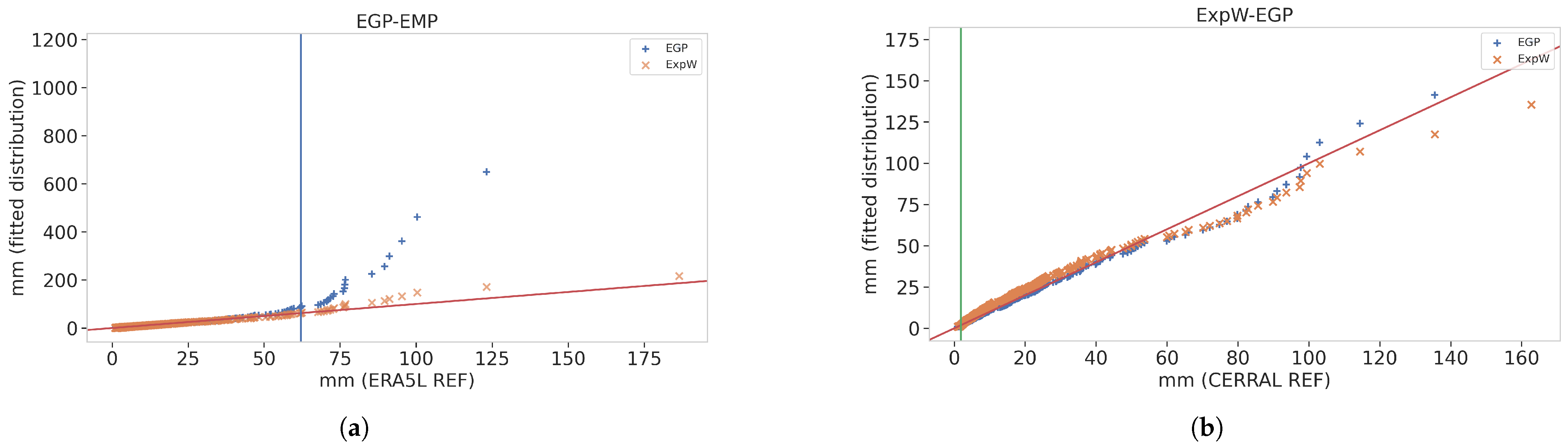
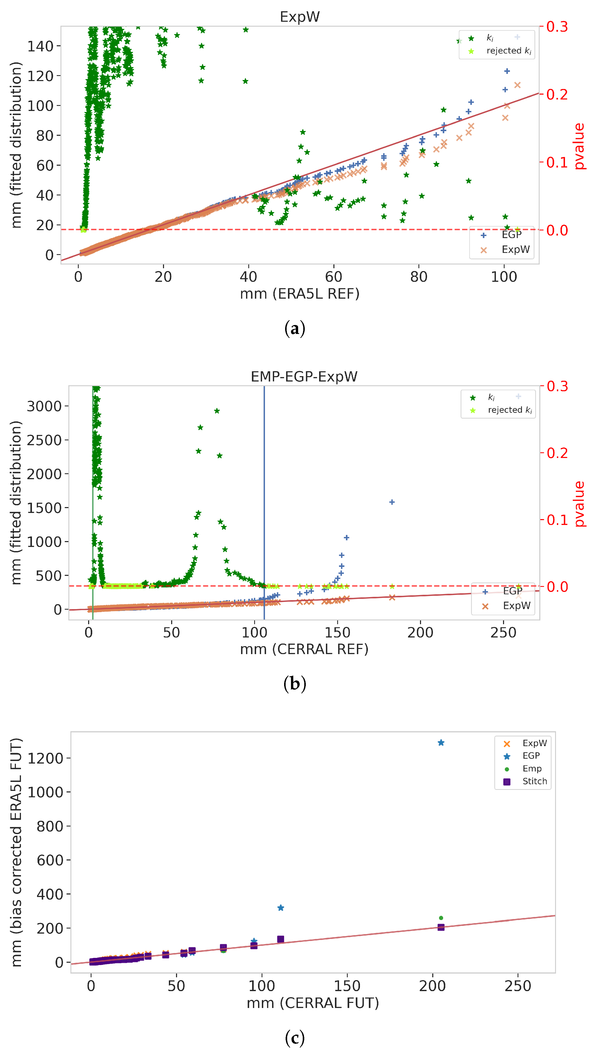
3.1. Stitch-BJ Fitting Results

Using the methodology presented in Section 2.3, we fitted the Stitch-BJ model to the daily precipitation data of ERA5L and CERRAL on the period 1 January 1985 to 31 December 2009. From these fitted models, both a spatial analysis of the stitching type and a global analysis of the stitching proportion can be obtained in Figure 6 and Figure 7.
Figure 6 shows what kind of stitch was performed for each location. None, left, right, left-right and full mean respectively no stitching, stitching of the lower tail, stitching of the upper tail, stitching of both tails or full replacement of the original EGP distribution.
For both the DJF and JJA seasons on ERA5L, the vast majority (resp 86.4% and 62.3%) of locations used a pure EGP distribution as shown in Figure 6 panels (a, b) with no replacement or stitching performed. This shows that most locations were able to get a satisfying fit out of purely parametric distributions. Stitching on the lower tail was performed on 10.1% and 35.5% of the locations, while the upper tail stitching affected respectively 3.4% and 2.0% of the locations. Full replacement of the original EGP distribution, as well as replacement of both tails, only affected 0.1% of the locations for both seasons.
For CERRAL data in panels (c, d), replacement proportions are similar, with 88.9% and 84.0% of the locations using a pure EGP distribution for the DJF and JJA seasons, respectively. Fewer locations required a lower tail replacement with 8.62% and 14.9% of the locations. The upper tail replacement affected 1.9% and 1.0% of locations, while replacements of both tails were involved in 0.4% and 0.0% of the locations. Full replacement of the EGP on CERRAL was used on 0.2% and 0.1% of the locations, respectively.
Maps of full details on the distributions used in the Stitch-BJ model are available in Figure A1 from Appendix A.
For locations where Stitch-BJ was used, one might want to know how much of the original distributions the stitching replaced. Overall, the median replacement affected 5% of the distribution for the lower tail, and less than 1% for the upper tail. More details can be found in Figure 7 with boxplots of the percentage of replacement for the lower and upper tail per season, for respectively ERA5L (panels a and c) and CERRAL (panels b and d). The lower replacement index i l concerned a larger portion of the distribution compared to i u but its impact is much smaller due to the small intensity of the rain affected. Overall, the i l for CERRAL were smaller, both for the median and outliers, than for ERA5L throughout all seasons. For the upper tail index i u , similar observations can be made with the CERRAL upper replacement portion being roughly equal to or lower than for ERA5L. This means that for locations where the EGP model misfitted small precipitations, up to 60% of the distribution’s lower tail was replaced. However, even at such a high proportion, the affected daily precipitation intensity remained relatively small. On the other hand, when the model misfitted the upper tail and extreme precipitation intensity, the replacement was only performed on less than 3% of the distribution for most locations, keeping as much of the original distribution’s upper tail as possible.
The Stitch-BJ model is heavily flexible, allowing it to automatically replace a portion of the EGP distribution with other models, either parametric or empirical, using p-value results from the PBJ goodness-of-fit statistical tests. This allows for a better fit to precipitation distribution, which can be extremely variable depending on the season and the location chosen.
Next, bias correction performances of all methods will be assessed using the CERRA-L validation period (1 January 2010 to 31 December 2020).

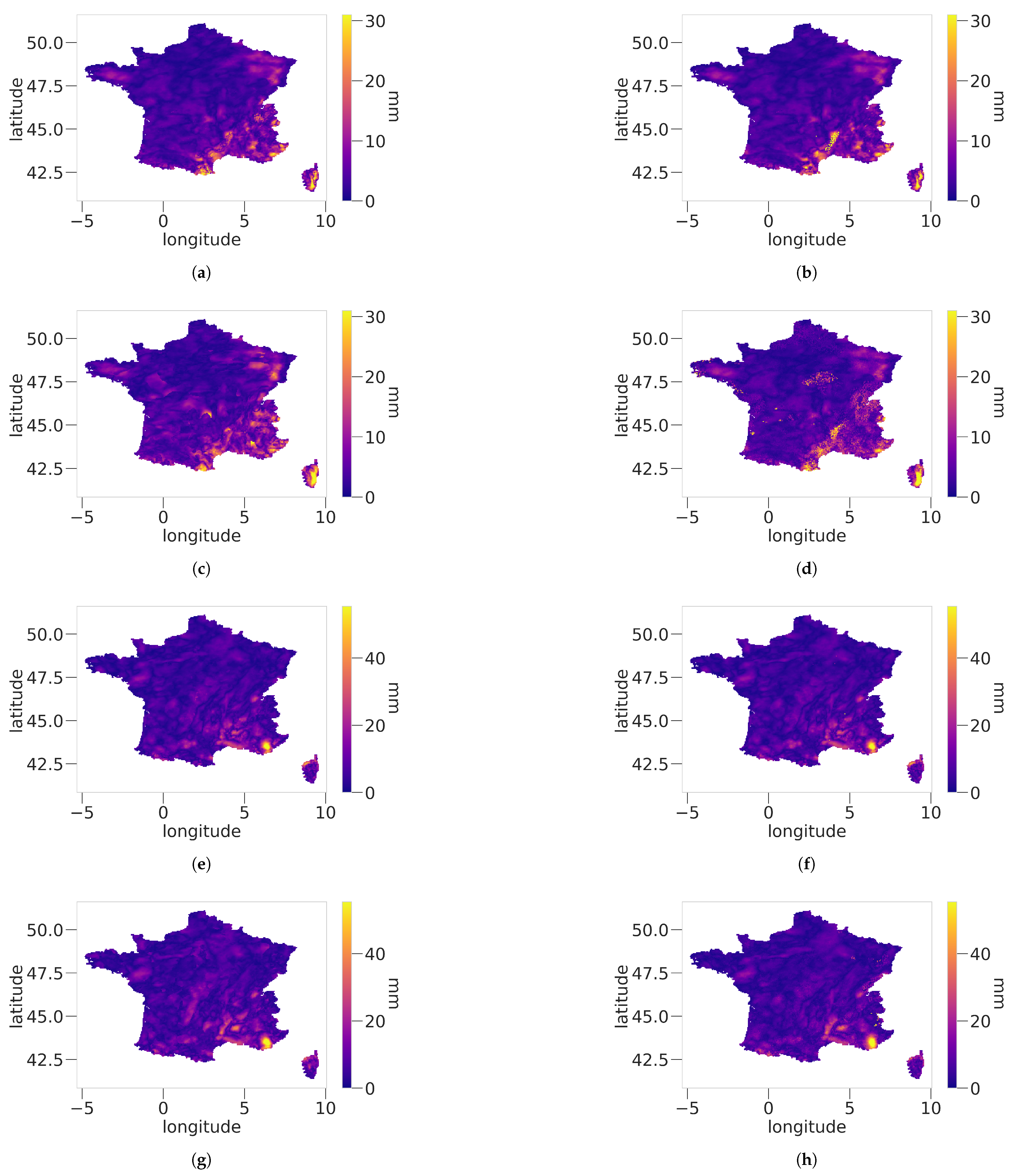
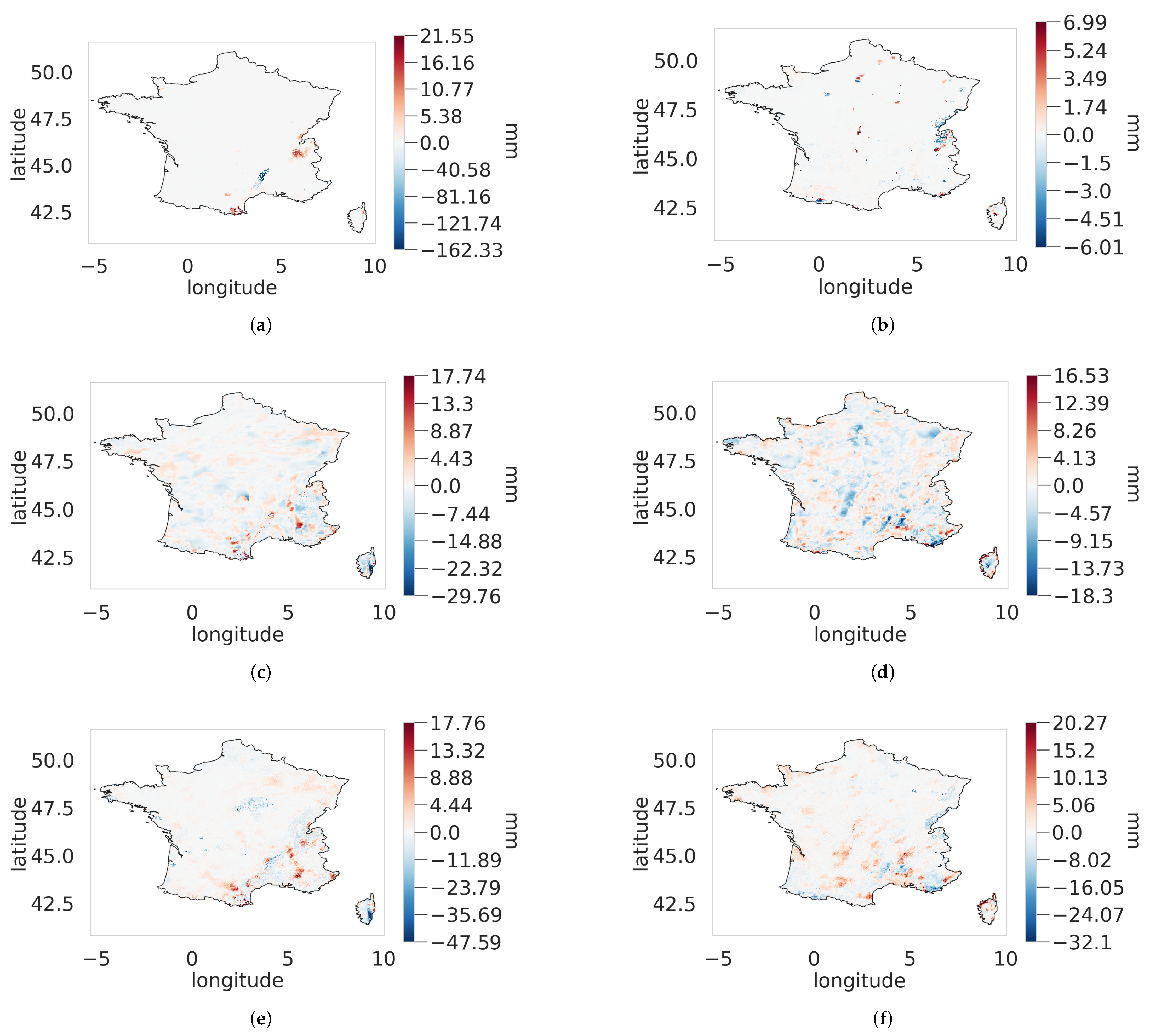
3.2. Bias Correction Results on the Period 2010–2020 and Interpretation

In this section, we compare the performance of the newly introduced Stitch-BJ against classical parametric distributions (EGP, ExpW, Gamma) and the empirical distribution (referred to as emp).
As explained in Section 2.1, both datasets ERA5L and CERRAL were first mapped on the same regular longitude/latitude grid (approximately 0.05 ° × 0.05 ° ), and the following periods have been used for training and validation:
  • Training period: 1 January 1985 to 31 December 2009;
  • Validation period: 1 January 2010 to 31 December 2020;
along with a separation using the meteorological seasons. Only the results of the correction of the validation period are shown in this section as they are similar to the ones from the previous study. In this section, the following metrics were computed on a pixel-by-pixel basis, and we noted q i n the quantile i n of the empirical distribution of the target data, i.e., F n 1 ( i n ) , and q i F the same quantile for a given distribution F, i.e., F 1 ( i n ) .
Mean Absolute Error
M A E F = 1 n i = 1 n | q i F q i n | .
Mean Absolute Error over the 95th percentile
M A E 95 s u p F = 1 n 95 % × n i = 95 % × n n | q i F q i n | ,
where · is the ceiling function.
Root Mean Squared Error
R M S E F = 1 n i = 1 n ( q i F q i n ) 2 .
The number of quantiles n was chosen to be 50 to ensure all locations had enough wet days without giving an artificially high weight to extremes.
Differences in metrics were also computed to increase visibility on the spatial improvements of one distribution over another. For two distributional models F and G, we compute the difference metrics as follows:
M A E d i f f F , G = M A E F M A E G , M A E 95 s u p d i f f F , G = M A E 95 s u p F M A E 95 s u p G , R M S E d i f f F , G = R M S E F R M S E G .
Note that in the following sections, Gamma’s error maps will not be shown. We will display only Gamma’s results in boxplots due to the very high errors. We do include the interpolated but non-corrected future model data for some figures, which are referred to as ERA5L in the legends. Moreover, the color ranges are fixed between maps of the same metrics to represent the 99.9th quantile error of the Stitch-BJ method. Finally, for differences in metrics, the scale is not fixed and may vary from distribution to distribution.

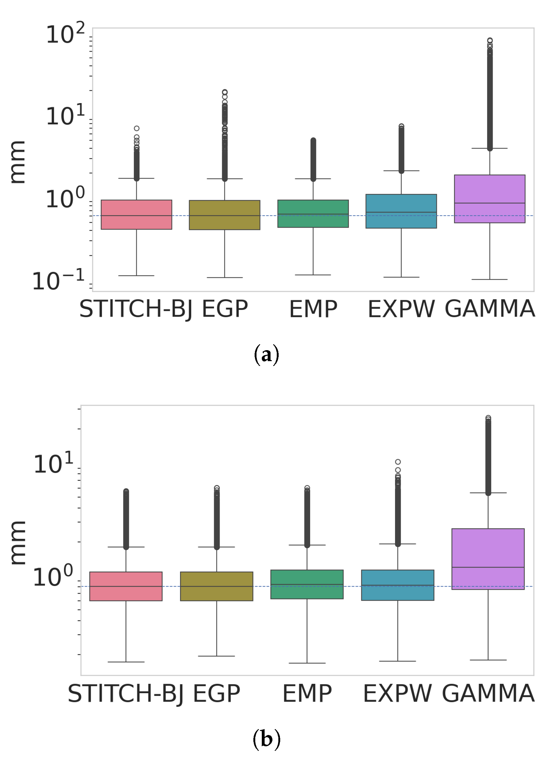
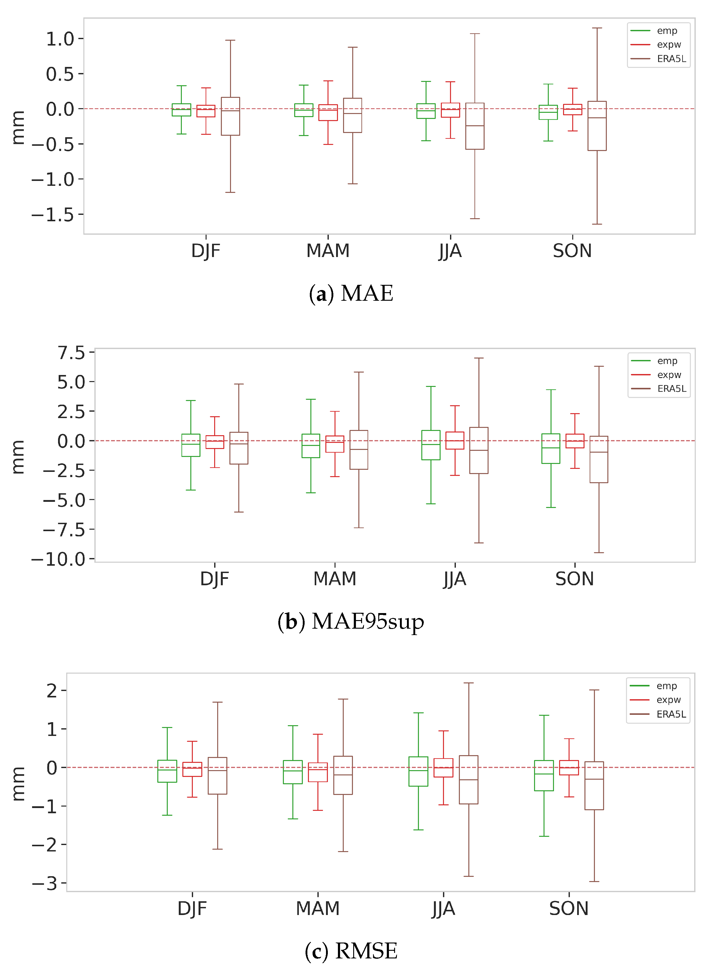
3.2.1. Mean Absolute Error

Differences of MAE for the bias correction performance shown in Figure 8 are quite difficult to assess. Both the spatial pattern and intensity of error are very similar for all chosen distributions. However, some extreme MAE for the EGP and ExpW models can be seen for the DJF season (panels b and c), respectively, near the Cévènnes and the Alps region. Those mountainous areas are known to be difficult to model due to their strong orographic features, paired with intense rain events during the SON and DJF seasons. Performances for the JJA season (panels e, f, g and h) are mostly identical, which may be caused by the lower amount of rain and fewer extreme events.
Differences maps in Figure 9 allow us to see where the Stitch-BJ provides a better correction, compared to the EGP and ExpW. We refer to model-season the error maps corresponding to the differences between Stitch-BJ’s error and model’s error, for the given season.
For the EGP-DJF (panel a), the EGP is at most 1.46 mm of MAE better than the Stitch-BJ, while an important increase in performance around the Cévènnes region, with a difference of more than 10 mm in terms of MAE in favor of the Stitch-BJ model. For EGP-JJA (panel b), performances are relatively similar between the Stitch-BJ and the EGP models.
For the ExpW-DJF (panel e), improvements cover a greater area but are less important with at most an improvement of the MAE of 5 mm while the ExpW improved at best the MAE of 1.3 mm. For the JJA season, the ExpW model improved at best 1.28 mm while the Stitch-BJ improved some locations by more than 5 mm. As for the emp-DJF and emp-JJA (panels c and d), improvements are much less important, and performance is relatively equal, with no models improving significantly over the other, with both models improving at most by approximately 1 mm.
From Figure 9, the impact of the stitching can be mostly seen around the Cévènnes, where the EGP has been improved upon by a great margin. However, we can also detect some locations around the northern Alps and the eastern Pyrenees where the stitching slightly worsened the performances. However, the tradeoff is still advantageous for the Stitch-BJ model.
A summary of statistics (mean, minimum, maximum, 25th, 50th and 75th percentile) of the MAE differences from Figure 9 are available in Table 3. We see that against all models, the Stitch-BJ was able to improve or perform similarly on the MAE, with the median being equal or below 0, and the 25th percentile always being higher (in absolute value) than the 75th percentile, meaning that globally, improvements on MAE are higher when using the Stitch-BJ compared to the other distributions. However, a small advantage of the empirical distribution over the Stitch-BJ can be seen for the DJF season on the maximum improvements, with a 2.82 mm maximum improvement for the Stitch-BJ and a 4.07 mm maximum improvement for the empirical distribution.
Boxplots of Figure 10 show how extreme errors are reduced for both the DJF and JJA seasons by using the Stitch-BJ model to replace misfitted portions of the EGP and ExpW distributions. For the DJF season (panel a), the Stitch-BJ was able to improve on the extreme error of both the EGP and ExpW distributions but fail to reduce the maximum error against the empirical distribution. However, the bulk of the outliers are essentially identical for the Stitch-BJ and the empirical distribution. Moreover, in terms of median MAE, the Stitch-BJ and EGP are improving against both the ExpW and empirical models (with an MAE of 0.61, 0.61, 0.64 and 0.67 for the Stitch-BJ, EGP, emp and ExpW, respectively). For the JJA season (panel b), conclusions are similar to the DJF season, but to a lesser extent, with much less extreme outliers produced by the EGP and ExpW distributions. All models are relatively competitive for the JJA season, and the Stitch-BJ and EGP still produce a very slightly lower median MAE than other models.

3.2.2. Mean Absolute Error over the 95th Percentile
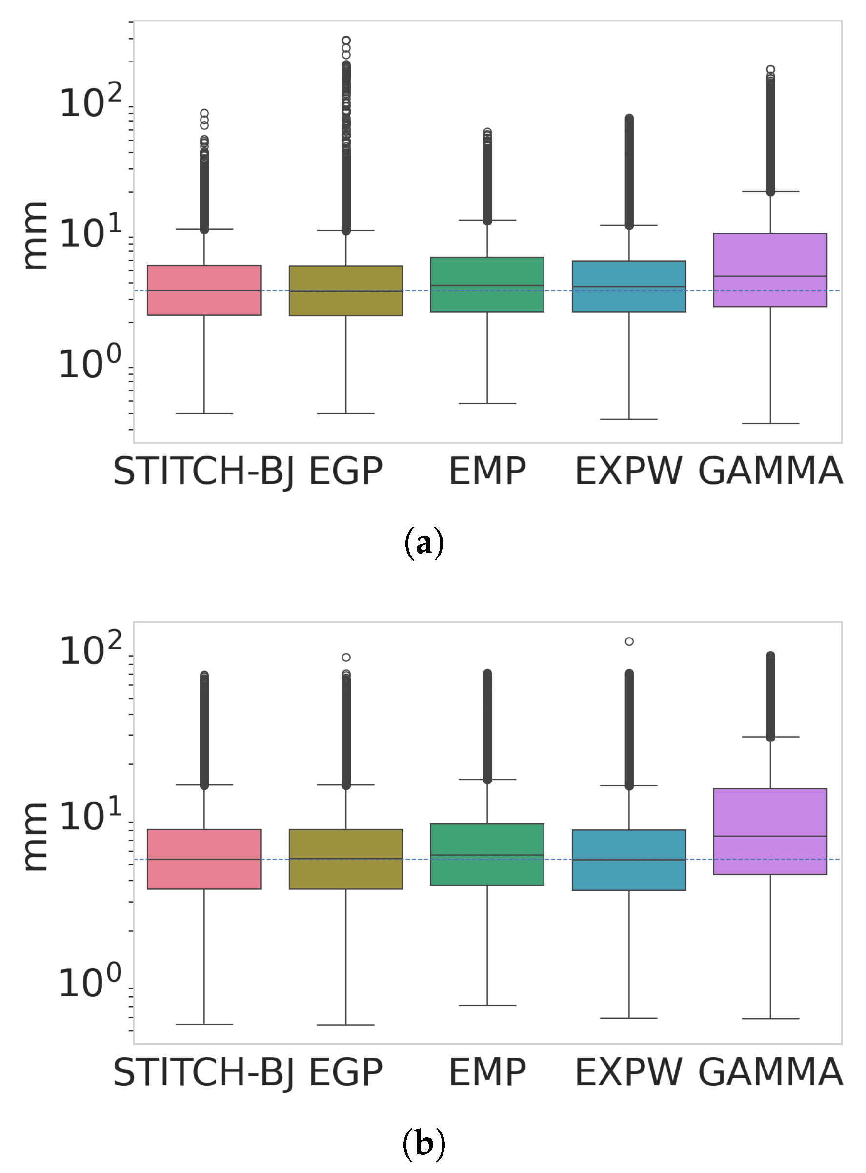
MAE95sup maps in Figure 11 are very similar to the MAE maps of Figure 8. However, for the DJF season, the Stitch-BJ was able to improve against all other shown models significantly in some regions: the Cévènnes and Corsica regions for both EGP and ExpW (panels a and c) and the Alps and Corsica regions for the empirical model (panel b). However, for the JJA season (panels d, e and f), no significant improvements are easily noticeable.
Differences of MAE95sup in Figure 12 clearly show the advantages of the Stitch-BJ against all other methods for the DJF season, mainly focused on the Cévènnes and Corsica region, with errors differences ranging from 30 mm to 162 mm (panels a, c and e). However, some locations show poor performance from the Stitch-BJ compared to other models, especially in the Eastern Pyrenees, where other models produce MAE95sup 17 mm to 21 mm lower. For the JJA season, performance is equivalent for most models (panels b and d), with only against the ExpW (panel f) where the Stitch-BJ can show higher improvements than the opposite with a maximum improvement of 32 mm against 20 mm for the ExpW.
A summary of statistics of the MAE95sup differences from Figure 12 are available in Table 4. Similarly to Table 3, improvements are noticeable when looking at the median, 25th and 75th percentile of MAE95sup differences for all models. Maximum improvements are higher for the Stitch-BJ against all models except for the empirical distributions which can be detected in the outliers of Figure 13.
In Figure 13, boxplots for the DJF season (panel a) shows a clear improvement in the Stitch-BJ against the EGP and ExpW models. At first glance, the ExpW model produces lower outliers than the Stitch-BJ, but this is only true for the three most extreme outliers produced by the Stitch-BJ. The rest of the outliers are much more condensed and generally lower than both the ExpW and empirical models’ outliers. Median errors are also slightly lower for the EGP and Stitch-BJ models compared to all other models for the DJF season. Models over the JJA season (panel b) produce very similar extreme outliers, and median errors are also very close and higher than for DJF.

3.2.3. RMSE

Maps from Figure 14 are very similar to the one for the MAE95sup in Figure 11, with mostly similar results for the DJF season except for the Cévènnes, Corsica and Alps region where the Stitch-BJ may perform better than the other models. For the JJA season, performances are very similar among all models.
In Figure 15, spatial patterns and intensity of errors match the ones from Figure 12 for both seasons. The Stitch-BJ method offers an advantage over the DJF season for all methods, while the JJA season shows very close performance for all models.
A summary of statistics of the RMSE differences from Figure 15 are available in Table 5. Compared to Table 3 and Table 4, improvements are less noticeable, especially when looking at the differences against the ExpW and emp models. While median and quartiles are still in favor of the Stitch-BJ, maximum improvements are in favor of the empirical and ExpW models for the DJF season.
Given observations that are similar to those in the previous figures, the conclusions from RMSE boxplots of Figure 16 are almost identical to Figure 13, with a slight improvement over median error for the Stitch-BJ and EGP models, and an improvement on extremes for the Stitch-BJ compared to the EGP and ExpW models for both seasons.

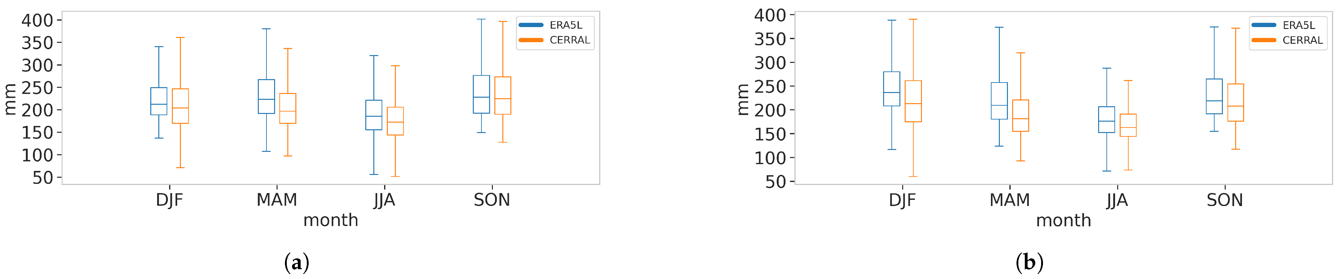
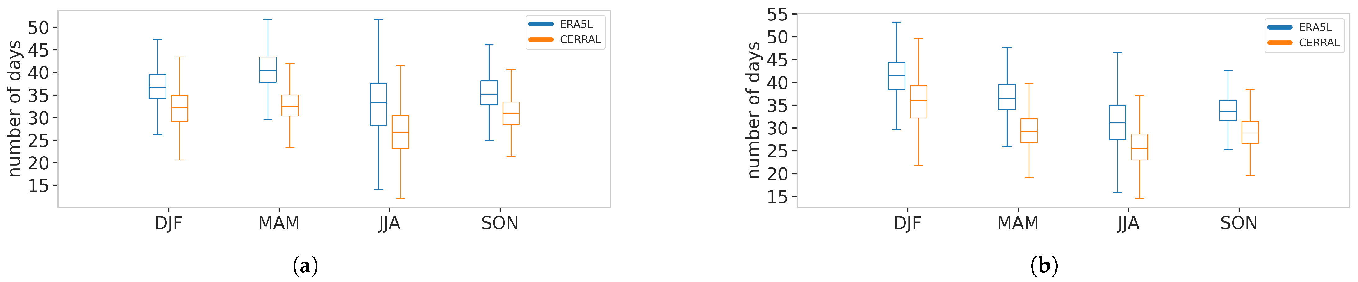
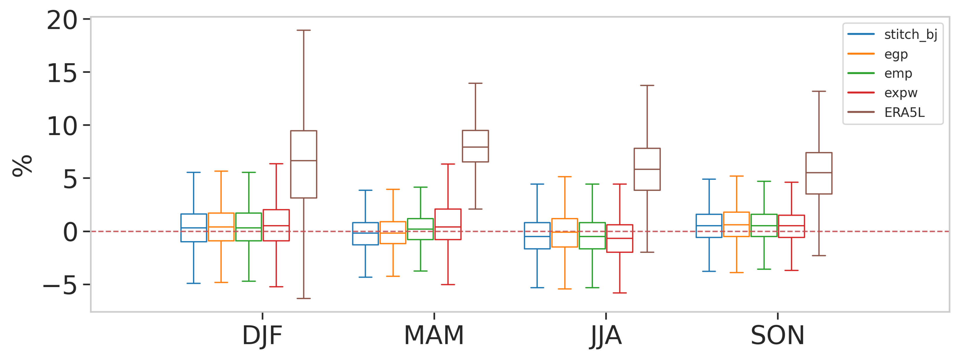
3.2.4. Impact of Seasonality on Performance

In the following figures, all seasons are shown on the same boxplot to assess the performance of the different methods season-wise. For the dry days’ probability in Figure 17, we show the difference between the target dry days probability and the modeled one: a positive value means a dry bias, while a negative one implies a wet bias.
In Figure 17, the impact of the SSR method is very noticeable for all seasons, with a large reduction in differences in dry days probability for all methods using the SSR correction. The method performed best for the DJF and MAM seasons, while a small wet bias remains in the JJA season and a dry bias in the SON season. Since the underlying model has almost no impact on the SSR correction, all models corrected with the SSR produce similar dry day probabilities.
For all metrics boxplots in Figure 18 and Figure 19, the M A E d i f f S t i t c h B J , m o d , M A E 95 s u p d i f f S t i t c h B J , m o d and R M S E d i f f S t i t c h B J , m o d (see Section 3.2) are shown with the EGP, ExpW and empirical distributions as competing models. A positive value means the competing model performed better, while a negative one means the Stitch-BJ performed better.
In Figure 18, we have seasonal boxplots of respectively the MAE, MAE95sup and RMSE differences in panels a, b and c. For the MAE differences in panel (a), the median differences are always negative and the first quartile is consistently lower than the third quartile for all seasons for the empirical and ExpW models. This means that the Stitch-BJ resulted in a lower median MAE for all seasons compared to all the other competing distributions. However, improvements on MAE are marginal, with the highest median improvement being for the SON season over the empirical distribution, which has an improvement of approximately 0.05 mm. As for the uncorrected model ERA5L, improvements are more noticeable, with median MAE differences being much lower than the others. We have similar observations in panel (b), with an improvement over the MAE95sup for all seasons over the empirical distribution. The ExpW model produces a median MAE95sup almost identical to the Stitch-BJ model for all seasons. This may be due to the ExpW being a flexible model as well, being able to model both light and heavy-tailed distributions. Results are constant throughout the seasons, with JJA and SON producing the most variations when compared with the empirical distribution. The empirical and uncorrected models were both outperformed in terms of median MAE95sup by the proposed model.
Similarly to Figure 18a,b, an improvement can be seen over the empirical method for the median differences in Figure 18c. A small improvement in the MAM season is noticeable against the ExpW, while performances are similar for all other seasons. The first and third quartiles are once again asymmetric, favoring the Stitch-BJ method slightly over the two others.
In Figure 19, we show the RMSE difference between the Stitch-BJ and EGP models, including outliers in the boxplot. We separated the EGP from the other distributions from Figure 16 to show the extent of the errors of the EGP without impacting the y-axis scale. For the MAM and JJA seasons, differences are quite symmetrical. This is expected due to the low replacement rate of the EGP for these seasons (see Figure 6). However, for the DJF and SON seasons, improvements provided by the Stitch-BJ model over the EGP model are much more noticeable. Many locations produced RMSE 100 to 600 mm higher than the Stitch-BJ location. This shows that even though most of the locations used the EGP to model the upper tail, the model cannot be used on all the study areas at the risk of producing extremely high errors. This emphasizes the importance of the considered Stitch-BJ model.

3.2.5. Local Analysis on a Selected Location

While Figure 4 gave an idea of how the stitching procedure worked, let us take a corrected location for a finer analysis. In Figure 20, we have quantile-quantile plots of the fitting procedure on both ERA5L and CERRAL data in panels (a, b), and the resulting bias-corrected data in panel (c). This location has been selected because it features multiple types of stitching and illustrates well the methodology used to produce the final Stitch-BJ model. In the PBJ test, p-values k i are produced and are used in the Stitch-BJ model to detect misfitted quantiles. When they cross a given threshold (red dashed line), we consider the corresponding quantile misfitted and we reject it. In the first two panels, dark green and light green stars correspond to the k i and rejected k i , respectively. The green and blue vertical lines correspond to the lower and upper rejection index i l and i u introduced in Section 2.3, and any quantiles lower (resp. higher) than the index are replaced with ones from another distribution. Basically, a different model is used for points being below (resp. above) the green (resp. blue) vertical line.
In Figure 20a, we have a local analysis where a full ExpW model has been used on ERA5L data. While the ExpW performed globally worse on high quantiles, the extreme errors of the EGP distribution (50 mm on the last quantile) resulted in the selection of the ExpW distribution as the final distributional model. Note that while rejected k i can be seen in the figure, since we completely replaced the distribution with an ExpW, no lower and upper stitching indexes are shown with vertical lines, meaning that the adopted model is a pure ExpW for this ERA5L’s location. In Figure 20b, a stitch distribution has been used for this location for CERRAL data. This specific stitch model is composed of an empirical distribution in the lower tail, an EGP distribution in the centre of the law, and an ExpW distribution in the upper tail. The notation associated is EMP-EGP-ExpW (see Figure 6).
This resulted in the bias correction qqplot in panel (c), where the Stitch-BJ is the best fitting model over all contenders. Moreover, we can see the impact of the stitch: if left as is, the EGP produced a large overestimation of almost 1000 mm for the highest quantile.
To put into perspective, for this location, the MAE is at respectively 1.1, 3.3, 4.1 and 25.6 mm for the Stitch-BJ, empirical, ExpW and EGP models. When considering the MAE95sup, which is more focused on the extremes, the errors are 6.3, 29.5, 17.0 and 440.0 mm respectively. For difference metrics, as shown in Figure 9, Figure 12 and Figure 15, the MAE differences are then respectively −2.2, −3.0 and −26.5 mm against the empirical, ExpW and EGP models. MAE95sup differences exhibit similar results with −23.2, −10.6 and −433.5 mm, respectively.
The analysis of Figure 20 shows how the stitching procedure can prevent extremely large errors from a misfitted EGP, and even improve upon the bias-corrected data using ExpW or the empirical distribution.

4. Discussion

This study presents a novel bias correction approach for seasonal daily precipitation data over France. The Stitch-BJ model leverages the strength of both parametric and empirical distributions for a more accurate representation of extremes.
The proposed approach combines a seasonal bias correction using the Stitch-BJ model with a dry-days frequencies correction using an adapted version for parametric distributions of the Singularity Stochastic Removal from [28], enabling the correction of both wet days intensity and dry days frequencies. However, in the case of a dry bias, the SSR method randomly adds wet days to the time series. While the added wet days are very low in intensity, this may impact the temporal autocorrelation of daily precipitation and bias some climate indicators such as the Cumulative Dry Day indicator.
In this study, the bias correction was applied seasonally using meteorological seasons (DJF, MAM, JJA, SON) to account for intra-annual non-stationarity. This allows us to adapt the distribution fittings to seasonal variations in precipitation regimes and climatology. However, this raises questions regarding the optimal number and definitions of seasons. Indeed, what is considered a season can greatly differ depending on the study area, and for a given area, can be impacted by climate change [64]. Some study applied bias correction method in a monthly manner to mitigate this issue [65], however in the case of parametric distributions, the limitation on training data can result in a poor fit for those models.
Despite overall robust performance, some limitations remain. Indeed, the current model relies on the EGP, ExpW and empirical distributions. However, the EGP and ExpW can be very similar, and the use of a different distribution for the tail may result in better performance. Additionally, performance in dry regimes or in low-precipitation months may be constrained due to the scarcity of data for reliable fitting, particularly in the upper tail.
Moreover, the present analysis shows a high sensitivity to extreme events. Depending on the user’s needs, the goal could be to produce worst-case scenarios and focus on capturing extremes, even if they are overestimated. In such cases, the models presented here could be useful. However, other users might want to be more conservative and avoid exaggerating results. For these users, there are various methods to reduce the sensitivity of the models to extreme values, such as removing [66,67] or adjusting the highest data points to avoid misfitting [24].
All metrics from this study were also solely based on quantiles of the wet days’ intensity distribution and on the proportion of dry days. Interesting results may arise from studying the impact of such models on climate indicators, which often consider the frequency and timing of such variables. Studying the impact on climate indicators also raises the question of multivariate bias correction as many indicators are issued from a combination of multiple climate variables. Most multivariate bias correction methods rely on a two-step procedure with a univariate bias correction of each climate variable first, then a correction of the correlation between variables [68,69]. Some interesting extensions would be on the application of the Stitch-BJ model on other climate variables, such as air temperature or wind speed, with the use of different distributions in the stitching procedure.
Finally, this study’s validation and training periods were all historical periods that could be compared with station data. However, climate projections, such as data from CMIP6, also need to be bias-corrected. Such data are influenced by greenhouse gas emission scenarios, which may greatly impact the likelihood of extreme events. Such settings may be better suited for parametric distributions for their ability to extrapolate to new extremes and would be an interesting future study to pursue, as in [70] or [71]. While the distributional models proposed here do not explicitly take into account climate change, multiple bias correction methods have been developed for bias correction in a climate change context such as the CDF-t [13] or the Quantile Delta Mapping [72].

5. Conclusions

In this study, our objective was to seasonally bias correct daily precipitation data from ERA5-Land with CERRA-Land data using out-of-sample validation. We applied the Stitch-BJ [26] model along with other distributions (see Section 2.3) combined with the Singularity Stochastic Removal method from [28] for to correct the probability of dry days. This allowed us to show the potential of parametric and semi-parametric bias correction methods against the classical empirical model.
We first showed the necessity of introducing a seasonal separation of our datasets in Section 2.1 and correcting the probability of dry days in Section 2.2. If left as is, residual bias would be left in the final result, which may worsen the performance of all models. To correct the dry-day probabilities of our models, we adapted the SSR method and applied it to semi- and fully-parametric models. This allowed us to obtain well-calibrated dry-day probabilities compared to uncorrected models, with differences with the target dry-day probabilities for the validation period of less than 0.01 across all seasons. Section 3.2.1 showed how the Stitch-BJ methodology adapted distributions locally to produce the best fitting model. This resulted in mostly parametric distributions across a variety of locations with heterogeneous properties, which allows for extrapolation to new extremes. In Section 3.2, we show the bias correction performance of all models for the DJF and JJA season across multiple metrics. We showed that the Stitch-BJ model produced performance similar to the empirical model in terms of MAE, with a slight reduction in the median error across the study area. For more extreme-focused metrics such as the MAE95sup or the RMSE, the Stitch-BJ model was able to show a reduction in extreme errors against all models for the DJF season, while performance was mostly equivalent for the JJA season. Again, median errors were lower for the Stitch-BJ compared to the empirical model, and error outliers were globally lower or similar to the empirical model’s. Comparing all seasons together, we do not see an impact on the relative performance of models against the Stitch-BJ, with the latter outperforming the ExpW and empirical models for all seasons.
Future work should investigate the model’s robustness in highly variable or evolving climates, particularly under climate change scenarios where the strengths of parametric distributions are expected to be most valuable. Extending the approach to additional climate variables and developing an open-source implementation would further increase its applicability for climate impact studies and operational services.

Author Contributions

Conceptualization, P.E., E.D.B., T.L., A.L. and M.T.; methodology, P.E., E.D.B. and T.L.; software, P.E.; validation, P.E., E.D.B. and T.L.; formal analysis, P.E.; investigation, P.E.; resources, P.E.; data curation, P.E.; writing—original draft preparation, P.E.; writing—review and editing, P.E., E.D.B. and T.L.; visualization, P.E.; supervision, E.D.B., T.L. and A.L.; project administration, E.D.B., T.L., A.L. and M.T.; funding acquisition, E.D.B., T.L., A.L. and M.T. All authors have read and agreed to the published version of the manuscript.

Funding

This work has been partially supported by the French government through the CIFRE funding (CIFRE No2022/0519) managed by the National Association of Research and Technology and the 3IA Côte d’Azur Investments in the Future project managed by the National Research Agency (ANR-19-P3IA-0002).

Institutional Review Board Statement

Not applicable.

Informed Consent Statement

Not applicable.

Data Availability Statement

All data, material, and programming codes used in this study are available upon request. ERA5-Land and CERRA-Land datasets analyzed in the current study are available on the Copernicus Climate Change Service (C3S) Climate Data Store https://cds.climate.copernicus.eu/ (accessed on 16 December 2024).

Conflicts of Interest

The Authors P.E., A.L. and M.T. were employed by the company Hydroclimat. The remaining authors declare that the research was conducted in the absence of any commercial or financial relationships that could be construed as a potential conflict of interest. The funders had no role in the design of the study; in the collection, analyses or interpretation of data; in the writing of the manuscript; or in the decision to publish the results.

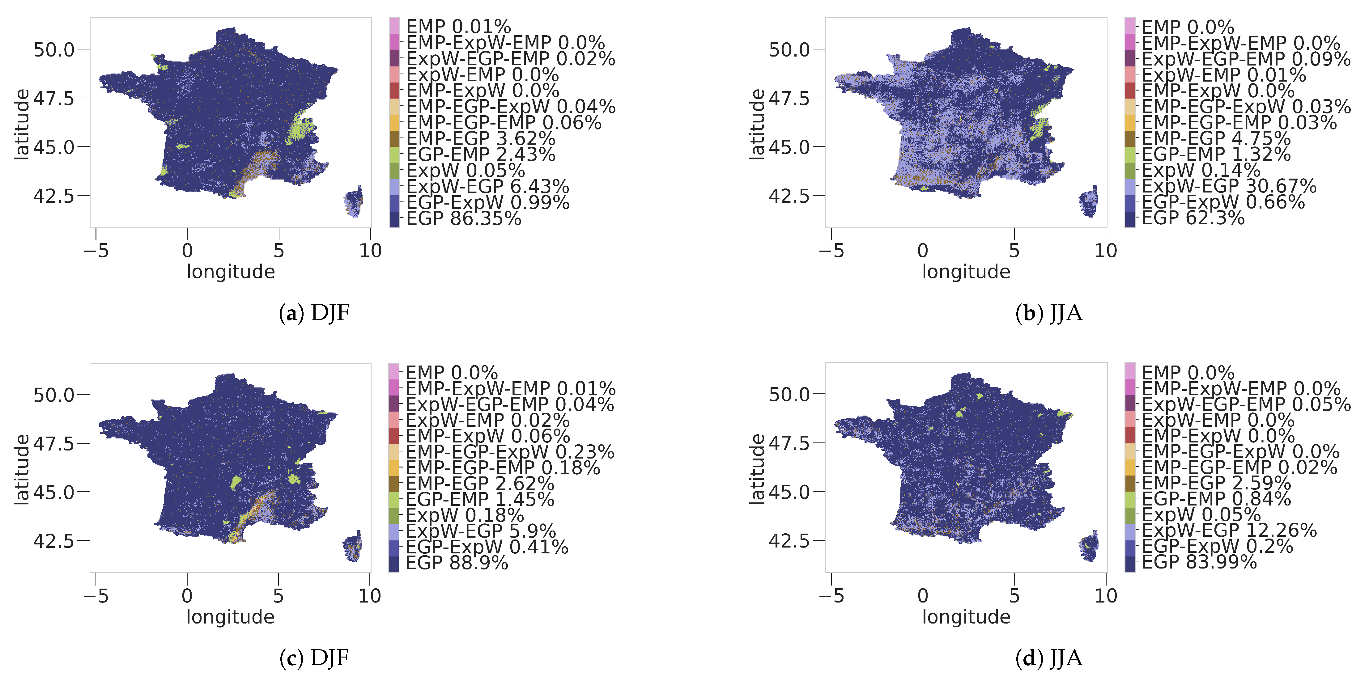
Appendix A. Full Stitching Maps for DJF and JJA Seasons on ERA5-Land and CERRA-Land for the Training Period

Figure A1. Detailed replacement map for the Stitch-BJ fitted on the reference period of ERA5L (a,b) and CERRAL (c,d) for DJF and JJA.
Atmosphere 16 00480 g0a1
Considering all fully parametric models, stitch between parametric models included, the proportion goes up to around 94% for both seasons. The remaining locations used mainly an empirical lower tail replacement (3.6% and 4.8% of the total locations respectively), while almost no locations used a purely empirical distribution. Spatially, most of the locations using the empirical distribution for either the lower or upper tail replacement are located in historically complex climate regions such as the Cévènnes, the Alps or the Corsica [73,74,75,76] due to their strong orographic charateristics. For the JJA season, these locations are a bit more spread out but still have a large concentration around the Alps and the Cévènnes, with some replacement along the Pyrénnées.
Replacement maps for CERRAL in Figure 6c,d are similar to those for ERA5L in panels (Figure 6a,b) with most of the locations for both DJF and JJA seasons using pure EGP distributions (88.9% and 84.0% respectively). The use of an empirical lower or upper tail is even rarer with respectively 95.4% and 96.5% of locations using a purely parametric distribution. Use of the empirical distribution for the upper tail is mainly located around the Cévènnes for the DJF season, while for JJA locations seems to be spread out on all the study areas. No locations used a fully empirical distribution for both DJF and JJA season while fitted on the CERRAL dataset.

References

  1. Casanueva, A.; Kotlarski, S.; Herrera, S.; Fernández, J.; Gutiérrez, J.M.; Boberg, F.; Colette, A.; Christensen, O.B.; Goergen, K.; Jacob, D.; et al. Daily precipitation statistics in a EURO-CORDEX RCM ensemble: Added value of raw and bias-corrected high-resolution simulations. Clim. Dyn. 2016, 47, 719–737. [Google Scholar] [CrossRef]
  2. Shayeghi, A.; Ziveh, A.R.; Bakhtar, A.; Teymoori, J.; Hanel, M.; Vargas Godoy, M.R.; Markonis, Y.; AghaKouchak, A. Assessing drought impacts on groundwater and agriculture in Iran using high-resolution precipitation and evapotranspiration products. J. Hydrol. 2024, 631, 130828. [Google Scholar] [CrossRef]
  3. Fosser, G.; Gaetani, M.; Kendon, E.J.; Adinolfi, M.; Ban, N.; Belušić, D.; Caillaud, C.; Careto, J.A.M.; Coppola, E.; Demory, M.E.; et al. Convection-permitting climate models offer more certain extreme rainfall projections. npj Clim. Atmos. Sci. 2024, 7, 1–10. [Google Scholar] [CrossRef]
  4. Alfieri, L.; Thielen, J. A European precipitation index for extreme rain-storm and flash flood early warning. Meteorol. Appl. 2015, 22, 3–13. [Google Scholar] [CrossRef]
  5. Sangati, M.; Borga, M. Influence of rainfall spatial resolution on flash flood modelling. Nat. Hazards Earth Syst. Sci. 2009, 9, 575–584. [Google Scholar] [CrossRef]
  6. Henckes, P.; Knaut, A.; Obermüller, F.; Frank, C. The benefit of long-term high resolution wind data for electricity system analysis. Energy 2018, 143, 934–942. [Google Scholar] [CrossRef]
  7. Prein, A.F.; Gobiet, A.; Truhetz, H.; Keuler, K.; Goergen, K.; Teichmann, C.; Fox Maule, C.; van Meijgaard, E.; Déqué, M.; Nikulin, G.; et al. Precipitation in the EURO-CORDEX 0.11° and 0.44° simulations: High resolution, high benefits? Clim. Dyn. 2016, 46, 383–412. [Google Scholar] [CrossRef]
  8. Wang, C.; Zhang, L.; Lee, S.K.; Wu, L.; Mechoso, C.R. A global perspective on CMIP5 climate model biases. Nat. Clim. Change 2014, 4, 201–205. [Google Scholar] [CrossRef]
  9. Şan, M.; Nacar, S.; Kankal, M.; Bayram, A. Daily precipitation performances of regression-based statistical downscaling models in a basin with mountain and semi-arid climates. Stoch. Environ. Res. Risk Assess. 2023, 37, 1431–1455. [Google Scholar] [CrossRef]
  10. Xu, H.; Xu, C.Y.; Sælthun, N.R.; Zhou, B.; Xu, Y. Evaluation of reanalysis and satellite-based precipitation datasets in driving hydrological models in a humid region of Southern China. Stoch. Environ. Res. Risk Assess. 2015, 29, 2003–2020. [Google Scholar] [CrossRef]
  11. Bador, M.; Boé, J.; Terray, L.; Alexander, L.V.; Baker, A.; Bellucci, A.; Haarsma, R.; Koenigk, T.; Moine, M.P.; Lohmann, K.; et al. Impact of Higher Spatial Atmospheric Resolution on Precipitation Extremes Over Land in Global Climate Models. J. Geophys. Res. Atmos. 2020, 125, e2019JD032184. [Google Scholar] [CrossRef]
  12. Déqué, M. Frequency of precipitation and temperature extremes over France in an anthropogenic scenario: Model results and statistical correction according to observed values. Glob. Planet. Change 2007, 57, 16–26. [Google Scholar] [CrossRef]
  13. Michelangeli, P.A.; Vrac, M.; Loukos, H. Probabilistic downscaling approaches: Application to wind cumulative distribution functions. Geophys. Res. Lett. 2009, 36. [Google Scholar] [CrossRef]
  14. Li, B.; Huang, Y.; Du, L.; Wang, D. Bias Correction for Precipitation Simulated by RegCM4 over the Upper Reaches of the Yangtze River Based on the Mixed Distribution Quantile Mapping Method. Atmosphere 2021, 12, 1566. [Google Scholar] [CrossRef]
  15. Naveau, P.; Huser, R.; Ribereau, P.; Hannart, A. Modeling jointly low, moderate, and heavy rainfall intensities without a threshold selection. Water Resour. Res. 2016, 52, 2753–2769. [Google Scholar] [CrossRef]
  16. Mamalakis, A.; Langousis, A.; Deidda, R.; Marrocu, M. A parametric approach for simultaneous bias correction and high-resolution downscaling of climate model rainfall. Water Resour. Res. 2017, 53, 2149–2170. [Google Scholar] [CrossRef]
  17. Velasquez, P.; Messmer, M.; Raible, C.C. A new bias-correction method for precipitation over complex terrain suitable for different climate states: A case study using WRF (version 3.8.1). Geosci. Model Dev. 2020, 13, 5007–5027. [Google Scholar] [CrossRef]
  18. Byun, K.; Hamlet, A.F. An improved empirical quantile mapping approach for bias correction of extreme values in climate model simulations. Environ. Res. Lett. 2024, 20, 014041. [Google Scholar] [CrossRef]
  19. Joly, D.; Brossard, T.; Cardot, H.; Cavailhes, J.; Hilal, M.; Wavresky, P. Les types de climats en France, une construction spatiale. Cybergeo Eur. J. Geogr. 2010. [Google Scholar] [CrossRef]
  20. Strohmenger, L.; Collet, L.; Andréassian, V.; Corre, L.; Rousset, F.; Thirel, G. Köppen-Geiger climate classification across France based on an ensemble of high-resolution climate projections. C. R. Géosci. 2024, 356, 67–82. [Google Scholar] [CrossRef]
  21. Boé, J.; Terray, L.; Habets, F.; Martin, E. Statistical and dynamical downscaling of the Seine basin climate for hydro-meteorological studies. Int. J. Climatol. 2007, 27, 1643–1655. [Google Scholar] [CrossRef]
  22. Derdour, S.; Ghenim, A.N.; Megnounif, A.; Tangang, F.; Chung, J.X.; Ayoub, A.B. Bias Correction and Evaluation of Precipitation Data from the CORDEX Regional Climate Model for Monitoring Climate Change in the Wadi Chemora Basin (Northeastern Algeria). Atmosphere 2022, 13, 1876. [Google Scholar] [CrossRef]
  23. Langousis, A.; Mamalakis, A.; Deidda, R.; Marrocu, M. Assessing the relative effectiveness of statistical downscaling and distribution mapping in reproducing rainfall statistics based on climate model results. Water Resour. Res. 2016, 52, 471–494. [Google Scholar] [CrossRef]
  24. Holthuijzen, M.; Beckage, B.; Clemins, P.J.; Higdon, D.; Winter, J.M. Robust bias-correction of precipitation extremes using a novel hybrid empirical quantile-mapping method: Advantages of a linear correction for extremes. Theor. Appl. Climatol. 2022, 149, 863–882. [Google Scholar] [CrossRef]
  25. Trentini, L.; Dal Gesso, S.; Venturini, M.; Guerrini, F.; Calmanti, S.; Petitta, M. A Novel Bias Correction Method for Extreme Events. Climate 2023, 11, 3. [Google Scholar] [CrossRef]
  26. Ear, P.; Di Bernardino, E.; Laloë, T.; Troin, M.; Lambert, A. A semi-parametric distribution stitch based on the Berk-Jones test for French daily precipitation bias correction. Stoch. Environ. Res. Risk Assess. 2025. to appear. [Google Scholar] [CrossRef]
  27. Katiraie-Boroujerdy, P.S.; Rahnamay Naeini, M.; Akbari Asanjan, A.; Chavoshian, A.; Hsu, K.l.; Sorooshian, S. Bias Correction of Satellite-Based Precipitation Estimations Using Quantile Mapping Approach in Different Climate Regions of Iran. Remote Sens. 2020, 12, 2102. [Google Scholar] [CrossRef]
  28. Vrac, M.; Noël, T.; Vautard, R. Bias correction of precipitation through Singularity Stochastic Removal: Because occurrences matter. J. Geophys. Res. Atmos. 2016, 121, 5237–5258. [Google Scholar] [CrossRef]
  29. Muñoz-Sabater, J.; Dutra, E.; Agustí-Panareda, A.; Albergel, C.; Arduini, G.; Balsamo, G.; Boussetta, S.; Choulga, M.; Harrigan, S.; Hersbach, H.; et al. ERA5-Land: A state-of-the-art global reanalysis dataset for land applications. Earth Syst. Sci. Data 2021, 13, 4349–4383. [Google Scholar] [CrossRef]
  30. Verrelle, A.; Glinton, M.; Bazile, E.; Moigne, P.L. CERRA-Land: A new land surface reanalysis at 5.5 km resolution over Europe. In Proceedings of the Copernicus Meetings, Virtual, 3–10 September 2021. [Google Scholar]
  31. Pelosi, A. Performance of the Copernicus European Regional Reanalysis (CERRA) dataset as proxy of ground-based agrometeorological data. Agric. Water Manag. 2023, 289, 108556. [Google Scholar] [CrossRef]
  32. Guo, C.; Ning, N.; Guo, H.; Tian, Y.; Bao, A.; De Maeyer, P. Does ERA5-Land Effectively Capture Extreme Precipitation in the Yellow River Basin? Atmosphere 2024, 15, 1254. [Google Scholar] [CrossRef]
  33. Gutiérrez, J.M.; Maraun, D.; Widmann, M.; Huth, R.; Hertig, E.; Benestad, R.; Roessler, O.; Wibig, J.; Wilcke, R.; Kotlarski, S.; et al. An intercomparison of a large ensemble of statistical downscaling methods over Europe: Results from the VALUE perfect predictor cross-validation experiment. Int. J. Climatol. 2019, 39, 3750–3785. [Google Scholar] [CrossRef]
  34. Reiter, P.; Gutjahr, O.; Schefczyk, L.; Heinemann, G.; Casper, M. Does applying quantile mapping to subsamples improve the bias correction of daily precipitation? Int. J. Climatol. 2018, 38, 1623–1633. [Google Scholar] [CrossRef]
  35. Chaouche, K.; Neppel, L.; Dieulin, C.; Pujol, N.; Ladouche, B.; Martin, E.; Salas, D.; Caballero, Y. Analyses of precipitation, temperature and evapotranspiration in a French Mediterranean region in the context of climate change. Comptes Rendus Geosci. 2010, 342, 234–243. [Google Scholar] [CrossRef]
  36. Braunstein, S.L. How large a sample is needed for the maximum likelihood estimator to be approximately Gaussian? J. Phys. A Math. Gen. 1992, 25, 3813. [Google Scholar] [CrossRef]
  37. Chen, D.; Dai, A.; Hall, A. The Convective-To-Total Precipitation Ratio and the “Drizzling” Bias in Climate Models. J. Geophys. Res. Atmos. 2021, 126, e2020JD034198. [Google Scholar] [CrossRef]
  38. Gutowski, W.J.; Decker, S.G.; Donavon, R.A.; Pan, Z.; Arritt, R.W.; Takle, E.S. Temporal–Spatial Scales of Observed and Simulated Precipitation in Central U.S. Climate. J. Clim. 2003, 16, 3841–3847. [Google Scholar] [CrossRef]
  39. Argüeso, D.; Evans, J.P.; Fita, L. Precipitation bias correction of very high resolution regional climate models. Hydrol. Earth Syst. Sci. 2013, 17, 4379–4388. [Google Scholar] [CrossRef]
  40. Maraun, D. Bias Correction, Quantile Mapping, and Downscaling: Revisiting the Inflation Issue. J. Clim. 2013, 26, 2137–2143. [Google Scholar] [CrossRef]
  41. Schmidli, J.; Frei, C.; Vidale, P.L. Downscaling from GCM precipitation: A benchmark for dynamical and statistical downscaling methods. Int. J. Climatol. 2006, 26, 679–689. [Google Scholar] [CrossRef]
  42. Lavaysse, C.; Vrac, M.; Drobinski, P.; Lengaigne, M.; Vischel, T. Statistical downscaling of the French Mediterranean climate: Assessment for present and projection in an anthropogenic scenario. Nat. Hazards Earth Syst. Sci. 2012, 12, 651–670. [Google Scholar] [CrossRef]
  43. Mao, G.; Vogl, S.; Laux, P.; Wagner, S.; Kunstmann, H. Stochastic bias correction of dynamically downscaled precipitation fields for Germany through Copula-based integration of gridded observation data. Hydrol. Earth Syst. Sci. 2015, 19, 1787–1806. [Google Scholar] [CrossRef]
  44. Piani, C.; Haerter, J.O.; Coppola, E. Statistical bias correction for daily precipitation in regional climate models over Europe. Theor. Appl. Climatol. 2010, 99, 187–192. [Google Scholar] [CrossRef]
  45. Vigaud, N.; Vrac, M.; Caballero, Y. Probabilistic downscaling of GCM scenarios over southern India. International Journal of Climatology 2013, 33, 1248–1263. [Google Scholar] [CrossRef]
  46. Semenov, M.A.; Brooks, R.J.; Barrow, E.M.; Richardson, C.W. Comparison of the WGEN and LARS-WG stochastic weather generators for diverse climates. Clim. Res. 1998, 10, 95–107. [Google Scholar] [CrossRef]
  47. Ambrosino, C.; Chandler, R.E.; Todd, M.C. Rainfall-derived growing season characteristics for agricultural impact assessments in South Africa. Theor. Appl. Climatol. 2014, 115, 411–426. [Google Scholar] [CrossRef]
  48. Vaittinada Ayar, P.; Vrac, M.; Bastin, S.; Carreau, J.; Déqué, M.; Gallardo, C. Intercomparison of statistical and dynamical downscaling models under the EURO- and MED-CORDEX initiative framework: Present climate evaluations. Clim. Dyn. 2016, 46, 1301–1329. [Google Scholar] [CrossRef]
  49. Bouvier, C.; Cisneros, L.; Dominguez, R.; Laborde, J.P.; Lebel, T. Generating rainfall fields using principal components (PC) decomposition of the covariance matrix: A case study in Mexico City. J. Hydrol. 2003, 278, 107–120. [Google Scholar] [CrossRef]
  50. Khan, S.; Kuhn, G.; Ganguly, A.R.; Erickson III, D.J.; Ostrouchov, G. Spatio-temporal variability of daily and weekly precipitation extremes in South America. Water Resour. Res. 2007, 43, W11424. [Google Scholar] [CrossRef]
  51. Abbott, T.H.; Stechmann, S.N.; Neelin, J.D. Long temporal autocorrelations in tropical precipitation data and spike train prototypes. Geophys. Res. Lett. 2016, 43, 11,472–11,480. [Google Scholar] [CrossRef]
  52. Themeßl, M.J.; Gobiet, A.; Heinrich, G. Empirical-statistical downscaling and error correction of regional climate models and its impact on the climate change signal. Clim. Change 2012, 112, 449–468. [Google Scholar] [CrossRef]
  53. Ajaaj, A.A.; Mishra, A.K.; Khan, A.A. Comparison of BIAS correction techniques for GPCC rainfall data in semi-arid climate. Stoch. Environ. Res. Risk Assess. 2016, 30, 1659–1675. [Google Scholar] [CrossRef]
  54. Lafon, T.; Dadson, S.; Buys, G.; Prudhomme, C. Bias correction of daily precipitation simulated by a regional climate model: A comparison of methods. Int. J. Climatol. 2013, 33, 1367–1381. [Google Scholar] [CrossRef]
  55. Martinez-Villalobos, C.; Neelin, J.D. Why Do Precipitation Intensities Tend to Follow Gamma Distributions? J. Atmos. Sci. 2019, 76, 3611–3631. [Google Scholar] [CrossRef]
  56. Husak, G.J.; Michaelsen, J.C.; Funk, C.C. Use of the Gamma distribution to represent monthly rainfall in Africa for drought monitoring applications. Int. J. Climatol. 2007, 27, 935–944. [Google Scholar] [CrossRef]
  57. Khan, S.A. Exponentiated Weibull regression for time-to-event data. Lifetime Data Anal. 2018, 24, 328–354. [Google Scholar] [CrossRef]
  58. Mudholkar, G.S.; Srivastava, D.K.; Kollia, G.D. A Generalization of the Weibull Distribution with Application to the Analysis of Survival Data. J. Am. Stat. Assoc. 1996, 91, 1575–1583. [Google Scholar] [CrossRef]
  59. Sharma, V.K.; Singh, S.V.; Shekhawat, K. Exponentiated Teissier distribution with increasing, decreasing and bathtub hazard functions. J. Appl. Stat. 2022, 49, 371–393. [Google Scholar] [CrossRef]
  60. Tencaliec, P.; Favre, A.C.; Naveau, P.; Prieur, C.; Nicolet, G. Flexible semiparametric Generalized Pareto modeling of the entire range of rainfall amount. Environmetrics 2019, 31, e2582:1. [Google Scholar] [CrossRef]
  61. Rivoire, P.; Martius, O.; Naveau, P. A Comparison of Moderate and Extreme ERA-5 Daily Precipitation With Two Observational Data Sets. Earth Space Sci. 2021, 8, e2020EA001633. [Google Scholar] [CrossRef]
  62. Haruna, A.; Blanchet, J.; Favre, A.C. Modeling Intensity-Duration-Frequency Curves for the Whole Range of Non-Zero Precipitation: A Comparison of Models. Water Resour. Res. 2023, 59, e2022WR033362. [Google Scholar] [CrossRef]
  63. Enayati, M.; Bozorg-Haddad, O.; Bazrafshan, J.; Hejabi, S.; Chu, X. Bias correction capabilities of quantile mapping methods for rainfall and temperature variables. J. Water Clim. Change 2021, 12, 401–419. [Google Scholar] [CrossRef]
  64. Wang, J.; Guan, Y.; Wu, L.; Guan, X.; Cai, W.; Huang, J.; Dong, W.; Zhang, B. Changing Lengths of the Four Seasons by Global Warming. Geophys. Res. Lett. 2021, 48, e2020GL091753. [Google Scholar] [CrossRef]
  65. Li, H.; Sheffield, J.; Wood, E.F. Bias correction of monthly precipitation and temperature fields from Intergovernmental Panel on Climate Change AR4 models using equidistant quantile matching. J. Geophys. Res. Atmos. 2010, 115, D10101. [Google Scholar] [CrossRef]
  66. Berg, P.; Bosshard, T.; Bozhinova, D.; Bärring, L.; Löw, J.; Nilsson, C.; Strandberg, G.; Södling, J.; Thuresson, J.; Wilcke, R.; et al. Robust handling of extremes in quantile mapping – “Murder your darlings”. Geosci. Model Dev. 2024, 17, 8173–8179. [Google Scholar] [CrossRef]
  67. Gutjahr, O.; Heinemann, G. Comparing precipitation bias correction methods for high-resolution regional climate simulations using COSMO-CLM. Theor. Appl. Climatol. 2013, 114, 511–529. [Google Scholar] [CrossRef]
  68. Cannon, A.J. Multivariate quantile mapping bias correction: An N-dimensional probability density function transform for climate model simulations of multiple variables. Clim. Dyn. 2018, 50, 31–49. [Google Scholar] [CrossRef]
  69. Vrac, M. Multivariate bias adjustment of high-dimensional climate simulations: The Rank Resampling for Distributions and Dependences (R2D2) bias correction. Hydrol. Earth Syst. Sci. 2018, 22, 3175–3196. [Google Scholar] [CrossRef]
  70. Andrade-Velázquez, M.; Montero-Martínez, M.J. Statistical Downscaling of Precipitation in the South and Southeast of Mexico. Climate 2023, 11, 186. [Google Scholar] [CrossRef]
  71. Enyew, F.B.; Sahlu, D.; Tarekegn, G.B.; Hama, S.; Debele, S.E. Performance Evaluation of CMIP6 Climate Model Projections for Precipitation and Temperature in the Upper Blue Nile Basin, Ethiopia. Climate 2024, 12, 169. [Google Scholar] [CrossRef]
  72. Cannon, A.J.; Sobie, S.R.; Murdock, T.Q. Bias Correction of GCM Precipitation by Quantile Mapping: How Well Do Methods Preserve Changes in Quantiles and Extremes? J. Clim. 2015, 28, 6938–6959. [Google Scholar] [CrossRef]
  73. Vautard, R.; Yiou, P.; Oldenborgh, G.J.v.; Lenderink, G.; Thao, S.; Ribes, A.; Planton, S.; Dubuisson, B.; Soubeyroux, J.M. Extreme Fall 2014 Precipitation in the Cévennes Mountains. Bull. Am. Meteorol. Soc. 2015. [Google Scholar] [CrossRef]
  74. Emmanuel, I.; Payrastre, O.; Andrieu, H.; Zuber, F. A method for assessing the influence of rainfall spatial variability on hydrograph modeling. First case study in the Cevennes Region, southern France. J. Hydrol. 2017, 555, 314–322. [Google Scholar] [CrossRef]
  75. Cortés-Hernández, V.E.; Caillaud, C.; Bellon, G.; Brisson, E.; Alias, A.; Lucas-Picher, P. Evaluation of the convection permitting regional climate model CNRM-AROME on the orographically complex island of Corsica. Clim. Dyn. 2024, 62, 4673–4696. [Google Scholar] [CrossRef]
  76. Estermann, R.; Rajczak, J.; Velasquez, P.; Lorenz, R.; Schär, C. Projections of Heavy Precipitation Characteristics Over the Greater Alpine Region Using a Kilometer–Scale Climate Model Ensemble. J. Geophys. Res. Atmos. 2025, 130, e2024JD040901. [Google Scholar] [CrossRef]
Figure 1. Yearly mean of seasonal cumulated precipitation for ERA5L and CERRAL over the training (a) and validation (b) periods.
Atmosphere 16 00480 g001
Figure 2. Yearly mean of number of wet days (>1 mm) for ERA5L and CERRAL per season for the training (a) and validation (b) periods.
Atmosphere 16 00480 g002
Figure 3. Boxplot of differences in probability of rain (days with >1 mm of rain) of ERA5L against CERRAL by season for the training (a) and validation (b) periods.
Atmosphere 16 00480 g003
Figure 4. Example of replacement indexes for the fitting of the Stitch-BJ model for a given location on ERA5L (a) and CERRAL (b) in the reference period (1 January 1985 to 31 December 2009).
Atmosphere 16 00480 g004
Figure 5. Basemap of France with the main cited regions in the study. The background represents the orography with white being the lowest elevation and dark brown the highest.
Atmosphere 16 00480 g005
Figure 6. Replacement map for the Stitch-BJ fitted on the reference period of ERA5L (a,b) and CERRAL (c,d) for DJF and JJA.
Atmosphere 16 00480 g006
Figure 7. Boxplots of percentages of the lower (first row) and upper tail (second row) being replaced by the stitching algorithm for ERA5L (a,c) and CERRAL (b,d).
Atmosphere 16 00480 g007
Figure 8. Maps of MAE for DJF (first and second rows) and JJA (third and fourth rows) for the following models: Stitch-BJ panels (a,e), EGP (b,f), emp (c,g) and ExpW (d,h).
Atmosphere 16 00480 g008
Figure 9. Maps of M A E d i f f S t i t c h B J , G for DJF (first column) and JJA (second column) with G being the following models: EGP (a,b), emp (c,d) and ExpW (e,f). Note that value ranges are specific to each map.
Atmosphere 16 00480 g009
Figure 10. Boxplots of MAE for DJF (a) and JJA (b) for all models. Note that the y-axis is in log10-scale.
Atmosphere 16 00480 g010
Figure 11. Maps of MAE95sup for DJF (first and second rows) and JJA (third and fourth rows) for the following models: Stitch-BJ (a,e), EGP (b,f), emp (c,g) and ExpW (d,h).
Atmosphere 16 00480 g011
Figure 12. Maps of M A E 95 s u p d i f f S t i t c h B J , G for DJF (first column) and JJA (second column) with G being the following models: EGP (a,b), emp (c,d) and ExpW (e,f). Note that value ranges are specific to each map.
Atmosphere 16 00480 g012
Figure 13. Boxplots of MAE95sup for DJF (a) and JJA (b) for all models. Note that the y-axis is in log10-scale.
Atmosphere 16 00480 g013
Figure 14. Maps of RMSE for DJF (first and second rows) and JJA (third and fourth rows) for the following models: Stitch-BJ (a,e), EGP (b,f), emp (c,g) and ExpW (d,h).
Atmosphere 16 00480 g014
Figure 15. Maps of R M S E d i f f S t i t c h B J , G for DJF (first column) and JJA (second column) with G being the following models: EGP (a,b), emp (c,d) and ExpW (e,f). Note that value ranges are specific to each map.
Atmosphere 16 00480 g015
Figure 16. Boxplots of RMSE for DJF (a) and JJA (b) for all models. Note that the y-axis is in log10-scale.
Atmosphere 16 00480 g016
Figure 17. Multi-season dry days probability difference between CERRAL and Stitch-BJ, EGP, emp, ExpW and uncorrected model ERA5L data.
Atmosphere 16 00480 g017
Figure 18. Multi-season MAE (a), MAE95sup (b) and RMSE (c) difference of Stitch-BJ, against emp, ExpW and uncorrected ERA5L. Note that outliers are not shown in these boxplots for readability.
Atmosphere 16 00480 g018
Figure 19. Multi-season RMSE difference between Stitch-BJ and EGP.
Atmosphere 16 00480 g019
Figure 20. Local analysis for location (Lon 9.3, Lat 41.96). (a) Fitting performance of the EGP and ExpW on ERA5L. (b) Fitting performance of the EGP and ExpW on CERRAL. (c) Bias correction performance for Stitch-BJ, EGP, ExpW and empirical model.
Atmosphere 16 00480 g020
Table 1. Proportion of rejected locations of the Student’s t-test for seasonal means differences. Note that values in bold correspond to ERA5L results, while values in italic correspond to CERRAL results.
DJFMAMJJASON
DJFx0.540.520.50
MAM0.50x0.350.80
JJA0.600.49x0.55
SON0.510.790.49x
Table 2. Proportion of rejected locations of the Student’s t-test for monthly means differences. Note that values in bold correspond to ERA5L results, while values in italic correspond to CERRAL results.
DJF123MAM123
1x0.050.321x0.330.26
20.10x0.1720.19x0.12
30.250.06x30.240.18x
JJA123SON123
1x0.110.111x0.140.30
20.17x0.0320.13x0.15
30.100.08x30.250.18x
Table 3. Spatially aggregated MAE differences statistics for all models for the DJF and JJA seasons.
DJF (JJA)EGP diffemp diffExpW diffGamma diff
mean−0.02 (−0.00)−0.02 (−0.04)−0.18 (−0.06)−1.36 (−1.20)
min−17.73 (−5.33)−2.82 (−2.37)−6.29 (−9.49)−82.20 (−24.09)
25th0.00 (−0.01)−0.10 (−0.14)−0.12 (−0.12)−1.14 (−1.63)
50th0.00 (0.00)−0.01 (−0.03)−0.02 (−0.02)−0.12 (−0.26)
75th0.00 (0.00)0.07 (0.07)0.05 (0.08)0.02 (0.00)
max4.19 (1.24)4.07 (2.22)3.43 (2.66)4.00 (3.05)
Table 4. Spatially aggregated MAE95sup differences statistics for all models for the DJF and JJA seasons.
DJF (JJA)EGP diffemp diffExpW diffGamma diff
mean−0.26 (−0.00)−0.55 (−0.49)−0.51 (−0.04)−5.39 (−4.89)
min−284.58 (−82.82)−42.87 (−27.88)−64.11 (−103.34)−169.05 (−63.91)
25th0.00 (−0.01)−1.35 (−1.63)−0.67 (−0.74)−4.50 (−6.60)
50th0.00 (0.00)−0.32 (−0.35)−0.06 (−0.02)−0.51 (−1.13)
75th0.00 (0.01)0.55 (0.86)0.41 (0.73)0.15 (0.27)
max69.58 (20.26)69.00 (39.99)63.60 (46.20)68.96 (51.49)
Table 5. Spatially aggregated RMSE differences statistics for all models for the DJF and JJA seasons.
DJF (JJA)EGP diffemp diffExpW diffGamma diff
mean−0.11 (0.00)−0.17 (−0.15)−0.23 (−0.04)−1.99 (−1.76)
min−110.71 (−30.28)−17.49 (−11.40)−23.73 (−36.74)−97.48 (−33.29)
25th0.00 (0.00)−0.39 (−0.49)−0.23 (−0.25)−1.62 (−2.40)
50th0.00 (0.00)−0.07 (−0.09)−0.02 (−0.01)−0.19 (−0.41)
75th0.00 (0.00)0.18 (0.27)0.13 (0.23)0.05 (0.06)
max29.22 (7.98)29.20 (13.49)27.06 (14.89)29.65 (16.69)
Disclaimer/Publisher’s Note: The statements, opinions and data contained in all publications are solely those of the individual author(s) and contributor(s) and not of MDPI and/or the editor(s). MDPI and/or the editor(s) disclaim responsibility for any injury to people or property resulting from any ideas, methods, instructions or products referred to in the content.

