Article

Biomass Burning over Africa: How to Explain the Differences Observed Between the Different Emission Inventories?

by
Toure E. N’Datchoh
1,*,
Cathy Liousse
2,
Laurent Roblou
2 and
A. Brigitte N’Dri
3
1
Laboratoire des Sciences de la Matière, de l’Environnement et de l’Energie Solaire (LASMES), UFR SSMT, University Félix, Houphouët-Boigny, Abidjan 22 BP 582, Côte d’Ivoire
2
Laboratoire d’Aérologie, UMR 5560, Toulouse, 14 Avenue Edouard Belin, 31400 Toulouse, France
3
Unité de Formation Sciences de la Nature (UFR-SN), Laboratoire d’Ecologie et de Développement Durable (LEDD), Laboratoire de Botanique et Valorisation de la Diversité Végétale (LaBVDiv), Université Nangui Abrogoua, Abidjan 02 BP 801, Côte d’Ivoire
*
Author to whom correspondence should be addressed.
Atmosphere 2025, 16(4), 440; https://doi.org/10.3390/atmos16040440
Submission received: 4 March 2025 / Revised: 3 April 2025 / Accepted: 6 April 2025 / Published: 10 April 2025
(This article belongs to the Section Air Quality)

Abstract

:
Biomass burning (BB) results from complex interactions between ecosystems, humans, and climate, releasing large amounts of gases and particles. Accurate BB emission estimates are essential for air quality, climate studies, and impact assessments. Various existing bottom-up BB emission inventories show significant discrepancies, varying by factors of 2 to 4 due to uncertainties in burned areas (BAs), emission factors (EFs), and vegetation parameters such as biomass density (BD) and burning efficiency (BE). Here, we investigate the role of vegetation parameters in these discrepancies in Africa. Two BB emission inventories, AMMABB-like (African Monsoon Multidisciplinary Analysis Biomass Burning) and GFED-like (Global Fire Emission Database) were developed for Organic Carbon (OC) and Black Carbon (BC). Both inventories used identical fire products, vegetation maps, and EF but different BD and BE values. Results highlight substantial differences in BD and BE, with relative gaps ranging from 44% to 85.12%, explaining the observed differences between BB emission inventories. Key vegetation classes responsible for BB emissions were identified. Discrepancies of 2.4 to 3.9 times were observed between AMMABB-like and GFED4-like, with higher values in the Southern Hemisphere. Better BD and BE estimates with regional distinctions for both hemispheres would improve BB emission accuracy in Africa.

1. Introduction

Biomass burning (BB) occurs in many vegetated ecosystems around the globe, with higher frequencies in the tropical and subtropical regions, which account for more than 50% of the total biomass burning. [1]. While BB is mainly used by populations in the tropical and subtropical regions [2,3,4], lightning is the main cause of vegetation fires in the boreal regions [5]. During all these fire events, important amounts of pollutants and trace gases are released into the atmosphere [6,7,8,9], resulting in poor air quality [10,11,12]. It is estimated that Africa alone is responsible for about 70% of the global burned area and about 50% of fire-related carbon emissions, mostly from savanna ecosystems [13,14]. It is also well known that BB emissions products can be transported over long ranges and can affect air quality thousands of kilometers away from the sources [15,16,17]. Numerous BB emission inventories exist [18,19] in the literature. Over the last decades, several studies have estimated BB emissions at both global and regional scales using either active fire, burned area from satellite products, or both [1,20,21,22,23,24]. Moreover, the estimation of biomass density is one of the main sources of uncertainties in the bottom-up emission inventories approach [25,26,27]. The ‘bottom-up’ approach consists of estimated emissions of BB from remote observation of burned area, active fire counts, and/or fire radiative power (FRP). These BB emissions are estimated by multiplying each biome-specific emission factor to convert each kilogram of burned dry matter to the amount of a trace gas or aerosol released into the atmosphere. However, large discrepancies exist in the BB emission inventories, particularly in Africa [23,28]. These discrepancies exist for both gas and particulate emissions, which are attributed to the methodology applied and/or the input data used, such as fire products, land cover, and emission factors. The well-known and widely used biomass-burning emission inventory in the scientific community remains the Global Fire Emission (GFED) inventory, which is based on the Moderate Resolution Imaging Spectroradiometer (MODIS) burnt area retrievals [1,29], as well as the Global Fire System (GFAS, [30]), based on the Fire Radiative Power (FPR) used as a default in the Copernicus Atmosphere Monitoring Service (CAMS) modeling framework.
However, using the L3JRC burned areas product [31], the African Monsoon Multidisciplinary Analysis Biomass Burning (AMMABB) inventory [28] presents 2.4 times greater emissions than those of GFEDv2 [32]. In addition, Nguyen and Wooster [23], using the “top-down” method of crossing fire radiative products and aerosol optical depth, found particulate matters, CO2, CO, and CH4 in their pan-African BB inventory to be higher than GFASv1.2 and GFEDv4 emissions inventories by approximately 114% and 69%, respectively. Whereas, in modeling studies, some of these existing emissions inventories need to be boosted by a factor varying from 2 to 4 for GFASv1.0 and 2 to 3.4 for GFASv1.2 to be able to reproduce observed Aerosol Optical Depths (AODs) [33,34,35]. The AMMABB inventory is able to reproduce the observed AODs without any boosting. GFED BB inventories are estimated using MODIS burned areas [36,37] and parameterizations in the Carnegie–Ames–Stanford Approach (CASA) biogeochemical model [38], which calculates plant productivity, tree mortality, leaf litter fall, and combustion completeness. This biogeochemical model uses 13 different vegetation classes defined from deciduous needle leaf to savanna, including urban and barren classes, as well as a prescribed vegetation map [39]. Emission factors used for this product are presented in Van Der Werf et al. [27] based on those suggested by Andreae and Merlet [40]. AMMABB inventories [28] were estimated using the L3JRC burned areas product from SPOT VEGETATION satellites at a spatial resolution of 1 km × 1 km [31]. A necessary correction of the burned areas related to the performance of that fire product over Africa was done before estimating these emissions [28]. The total emission for a given aerosol particle or gas is the result of a combination of burned area extent and vegetation cover from Global Land Cover (GLC) considering 21 vegetation types, with 14 allowing fire igniting and propagation [28], burning efficiency, and emission factors. Emission factors vary with vegetation type and are a combination of emission factors by Liousse et al. [41] for black carbon (BC) and organic carbon (OC), and Andreae and Merlet [40]. Full descriptions and details about the AMMABB inventory are given in Liousse et al. [28]. As mentioned above, the two inventories, GFED and AMMABB, using different burning area products, vegetation maps, burning efficiencies, and almost similar emission factors, obtained important differences between their BB emissions budget for Africa. Therefore, several questions were raised: are these huge gaps related to: (1) the methodology applied for each inventory? What is the importance of each parameter’s role in the biomass burning uncertainties over Africa? (2) burned area products? (3) vegetation maps? (4) burning efficiencies? (5) biomass density? Intercomparison efforts of global BB emissions inventories, using active fires and burned area products, also revealed large differences between inventories [22]. Moreover, when using BB emissions for air quality studies by models and satellite, notable differences were reported between gaseous and particulate pollutant values [42,43]. Slight differences (within 30% differences) between emissions inventories may be amplified in model simulations depending on the species and regions, with deviations up to 2–5 times, with higher signals in the southern hemisphere [42]. In addition, these differences in BB emissions inventories have important and significant impacts on aerosols’ radiative effects (direct, indirect, and semi-direct) assessments by models [43,44]. Therefore, it appears necessary to better understand the BB emissions inventories for regions such as Africa, where BB is a frequent practice [37,45] during the dry season [46,47], and its impact on air quality and climate [11,12,13]. This work aims to investigate and better understand the differences between two “bottom-up” inventories, namely AMMABB and GFED, with a focus on the role of vegetation parameters (biomass density (BD) and burning efficiency (BE)). For this purpose, two BB emission inventories called AMMABB-like and GFED-like have been developed using the same fire product, the same vegetation map, and the same emission factors, but with different BD and BE. This will allow for assessing the relative importance of BD and BE in the uncertainties and contributing to BB inventories’ improvement over Africa.

2. Materials and Methods

2.1. Methodology

The methodology applied here to develop AMMABB-like and GFED-like for BC and OC is similar to the methodology used for AMMABB inventories [28]. It is worth noting that this methodology can be used for any gas and particles emitted during a BB event. We choose to focus only on BC and OC here, mainly for brevity, as these particles directly impact air quality. For the reader’s understanding, a brief description of the methodology is provided here. The emission of the given species X derived from the burned area is estimated using the Seiler and Crutzen [6] formula:
E(X) = Σ(BAi × BDi × BEi × EFi (X))
where BA is the burned area (in m2), BD is the biomass density (in kg·m−2), BE is the burning efficiency, which is the amount of biomass effectively burned, and EF is the emission factor for the species X. “i” is the vegetation type. In order to focus on the role of vegetation parameters, EF(X) and BA are chosen to be the same for AMMABB-like and GFED-like, as well as the vegetation map (Global Land Cover map 2000, Figure 1), but BD and BE are different. Values for EF for both species BC and OC are provided by Liousse et al. [28]. The BA used in this study is from the Collection 5 MODIS burned area product (see Section 2.2). BD and BE are obtained from Liousse et al. [28] and Randerson et al. [29] for AMMABB-like and GFED-like, respectively. To facilitate comparison, the GFED vegetation parameters (BD and BE) were extracted from the GLC 2000 map. Table 1 summarizes the vegetation code and full name for each cover class of the GLC 2000 [48], as well as their corresponding BE and BD values for AMMABB-like and GFED-like developments. It is worth noting that BE values for both emission inventories are very close (in the same range), whereas BD values present high differences: this will be discussed in the results section. In this work, the relative difference between AMMABB-like and GFED-like was assessed using Equation (2):
R(Y) = 100 × (YAMMABB − YGFED) ÷ YAMMABB
where Y is the vegetation parameter (BE, BD, or BDBE) or the estimated emission of a given species based on values from the total AMMABB-like and GFED-like emissions estimated during this work.

2.2. Collection 5 MODIS Burned Area Product

Daily burned areas product from MODIS collection 5 at 500 m spatial resolution was used for fire emission estimations in Africa between 2001 and 2012 over the 6 African areas as shown in Figure 1. These data acquisition and processing are fully described by Roy et al. [49]; here, a brief description is given. Burned areas are characterized by charcoal and ash deposition, vegetation removal, and alteration [50,51]. These characteristics are used by the MODIS sensors to retrieve the burned area scars left after the fire occurrences. More details about the MODIS burned areas product can be found in the user manual [52].

2.3. Global Vegetation Cover Map

The Global Land Cover of the year 2000 (GLC2000, Figure 1) at 1 km spatial resolution was used to estimate the biomass burning emissions. The GLC2000 vegetation map was produced through the collaboration of 30 international research groups coordinated by the European Commission Joint Research Centre [53]. The land cover database was made based on daily data from the VEGETATION sensor on board SPOT 4. Details about the database accuracy and validation are described in Mayaux et al. [48].

3. Results

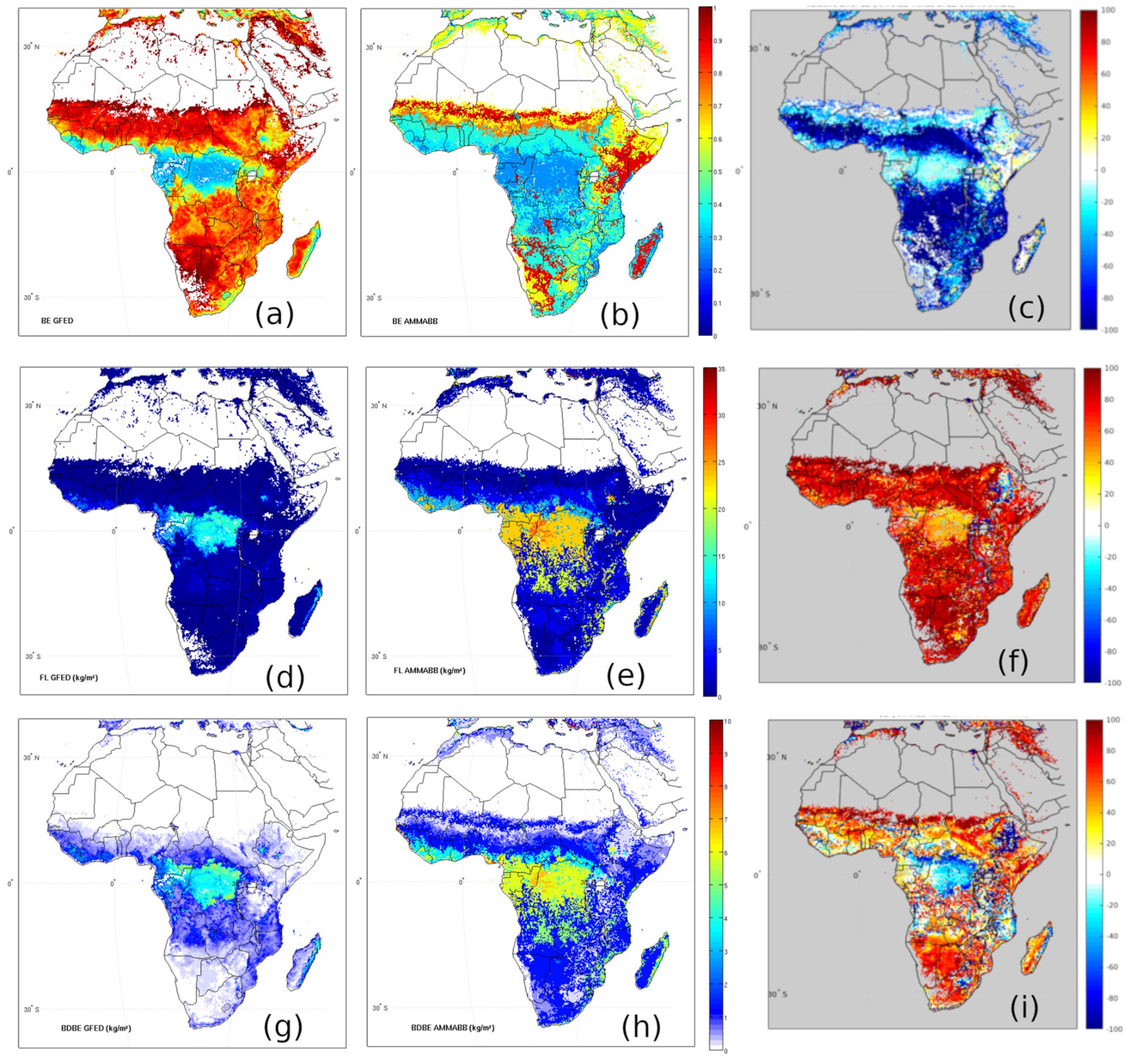
3.1. BE, BD Spatial Comparison

Burning Efficiency (BE), also called Combustion Completeness, and Biomass Density (BD, also known as fuel load) spatial distribution maps are shown in (Figure 2). BD and BE values from GFED (hereafter BDGFED, BEGFED) were available at the resolution of 0.25° × 0.25°. To facilitate comparison, the AMMABB BD and BE (hereafter BDAMMABB and BEAMMABB) values are defined for each vegetation type from the GLC vegetation map. Therefore, BDAMMABB and BEAMMABB used in Liousse et al. [28] were spatialized at 1 km × 1 km resolution using the GLC 2000 vegetation map according to vegetation classes with the Quantum Geographic Information System (QGIS) software. Also, by interpolation and intersection methodology in QGIS, the corresponding BD and BE values of GFEDv4 were extracted for each of the GLC vegetation classes. All values of BD, BE, and the product of BD by BE for both AMMABB and GFEDv4 can be seen in Table 1.
Figure 2a–c show the BEAMMABB, BEGFED, and their associated relative gaps in percentage spatial distribution over Africa. It can be observed that BEGFED is generally higher than BEAMMABB except in the Horn of Africa (Win11), where BEAMMABB is slightly higher (20%). Over central Africa (Win12) and the Sahelian region (Win10), BEGFED and BEAMMABB show close agreement. Differences are more pronounced in humid and dry savanna (5° N to 15° N; 5° S to 20° S and Horn of Africa) where BE relative gaps are found to be larger than 60% in absolute value, with higher values for GFED than AMMABB.
A summary of BEAMMABB/GFED ratios is provided in Table 1, revealing that these ratios vary from 0.350 (GLC 2: Tree cover Broadleaved deciduous Closed) to 1.923 (GLC 3: Tree cover Broadleaved deciduous Open). The spatial distribution of BDGFED, BDAMMABB, and their associated relative gaps in percentage (Figure 2d,e) showed significant differences. We found relative gaps above 60% almost everywhere except in the central part of Africa where these gaps are around 40%. This suggests that biomass density is more important in the AMMABB than in the GFED inventories. Table 1 revealed that BDAMMABB/GFED is between 0.207 (GLC 17: Mosaic Cropland/Tree Cover/Other Natural Vegetation) and 18.335 (GLC 2: Tree cover Broadleaved deciduous Closed). The product BE × BD is also known as fuel consumption and is referred to as “BEBD” hereafter. The spatial distribution of BEBDAMMABB, BEBDGFED, and their associated relative gaps is shown in Figure 2g–i. The only agreement between the fuel consumption values is found over the cultivated and managed area (GLC 16) with similar values of BEBD in both GFED and AMMABB (Table 1). The BEBDAMMABB are overall higher than BEBDGFED, from 1.795 for the Tree cover broadleaved Evergreen (GLC 1) to 9.189 for the Tree Cover, regularly flooded, saline water (GLC 8) vegetation classes. The spatial distribution of the relative gaps (Figure 2i) showed that over the Sahel (Win09) and the southern part of Africa (Win13), relative gaps are positive and higher than 60%. Negative relative gaps of more than 70% are observed over central Africa (Win12) and the Horn of Africa, i.e., from Ethiopia (Win11) to northern Kenya (Win12). This points out that the differences between GFED and AMMABB vegetation parameters need to be investigated for each vegetation type, and their contribution to total emissions assessed.

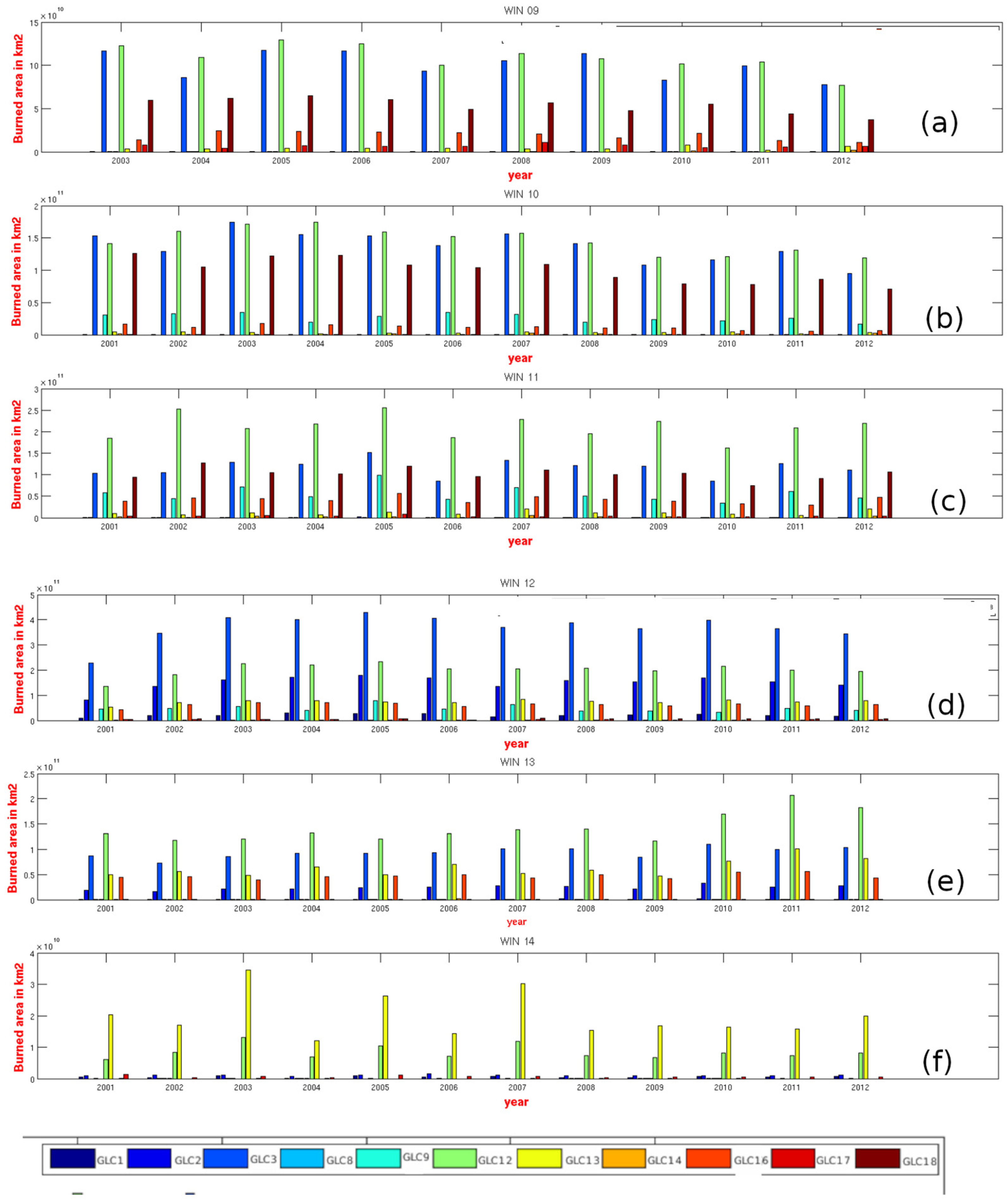
3.2. Frequently Burned Vegetation Types

This section is focused on the identification of the frequently burned vegetation types in Africa. As vegetation parameters highlighted important gaps between the AMMABB and GFED values depending on the vegetation class, it seems important to identify the most frequently burned vegetation types to understand their contributions to the existing gaps in BB emissions inventories. To achieve this, the GLC2000 vegetation map split by windows raster intersection areas with the year-to-year MODIS burned areas was calculated using QGIS between 2001 and 2012. For each burned pixel, detailed vegetation information (vegetation class) was recorded. From this vegetation burned information and BA, for each year, the total BA per vegetation type was estimated. Figure 3 presents the time series between 2001 and 2012 of total BA in km2 classified by vegetation class for each of the windows of the study area (Figure 1). Also, the mean proportion of each vegetation class burned compared to total burned vegetation was estimated for each window, and values are provided in Table 1.
From Figure 3 and Table 1, the main vegetation classes that are often burned in Africa, considering all windows, are GLC1 (Tree Cover, broadleaved, evergreen), GLC2 (Tree Cover, broadleaved, deciduous, closed), GLC3 (Tree Cover, broadleaved, deciduous, open), GLC8 (Tree Cover, regularly flooded, saline water), GLC9 (Tree cover/Other natural vegetation), GLC12 (Shrub Cover Closed-open, deciduous), GLC13 (Mosaic Tree Cover/Other Natural Vegetation), GLC14 (Sparse Herbaceous or Sparse Shrub Cover), GLC16 (Cultivated and managed areas), GLC17 (Cropland/Tree Cover/Other natural vegetation), and GLC18 (Cropland/Shrub or Grass Cover). However, these vegetation classes did not burn in a similar proportion for all the windows considered. When GLC3 (representing 34.21% of total mean burned vegetation), GLC12 (38.93% of total mean burned vegetation), and GLC18 (17.70% of total mean burned vegetation) were predominant over windows 9 (West Africa) and 10 (north-central Africa), GLC3 (28.54% of total mean burned vegetation), GLC12 (32.16% of total mean burned vegetation), GLC9 (10.47% of total mean burned vegetation), and GLC18 (25.28% of total mean burned vegetation) were dominant on windows 11 (East Africa). Over Windows 12 (Central Africa) and 13 (Southern Africa), GLC2 (18.04% and 8.84% of total mean burned vegetation, respectively), GLC3 (37.16% and 28.04% of total mean burned vegetation, respectively), GLC12 (22.16% and 33.95% of total mean burned vegetation, respectively), and GLC13 (6.99% and 10.86% of total mean burned vegetation, respectively) were predominant. Over window 14 (Madagascar), only GLC12 (31.67% of total mean burned vegetation) and GLC13 (58.57% of total mean burned vegetation) were predominant. Overall, there is a weak variability in the amount of burned area per vegetation type over the entire study area.

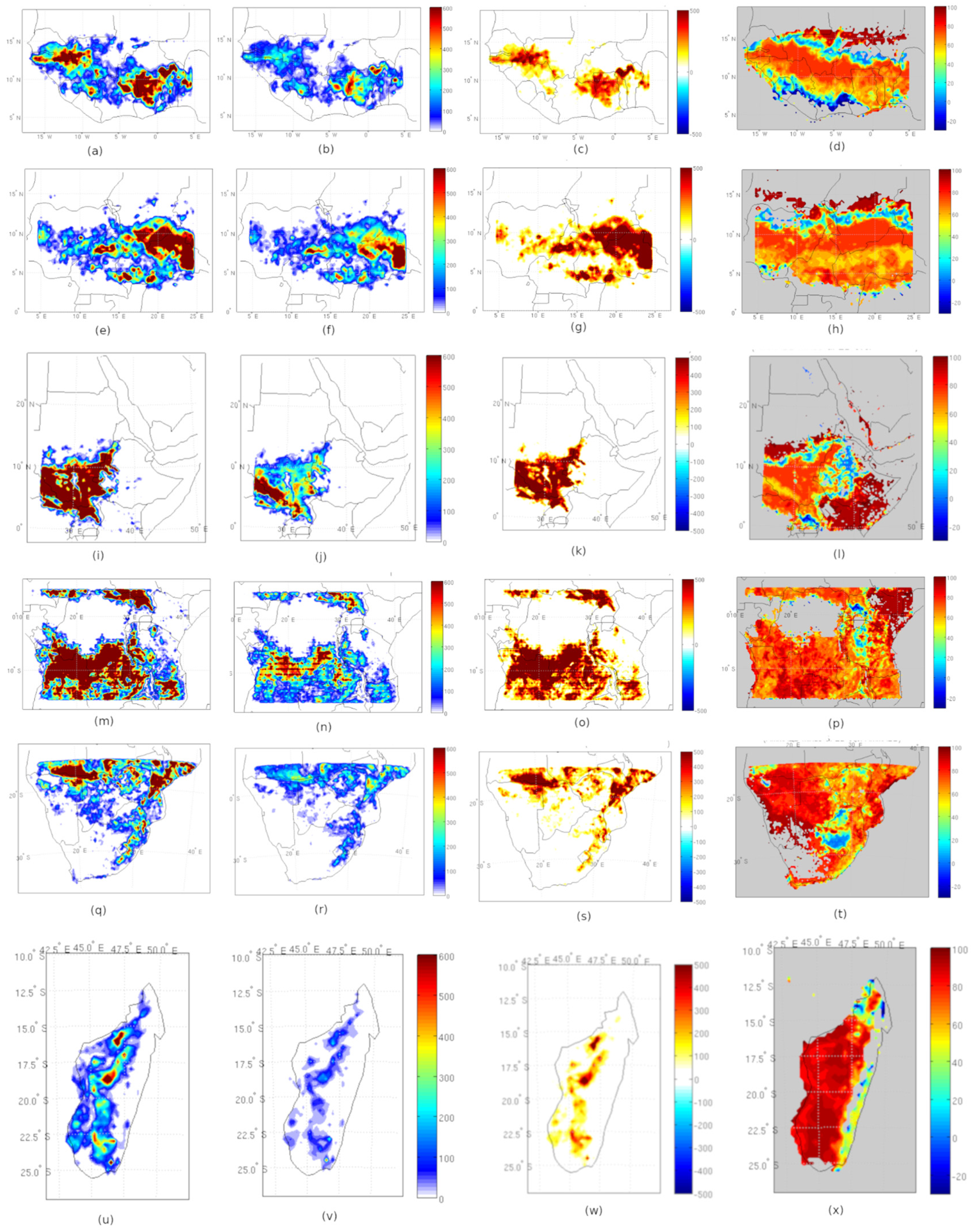
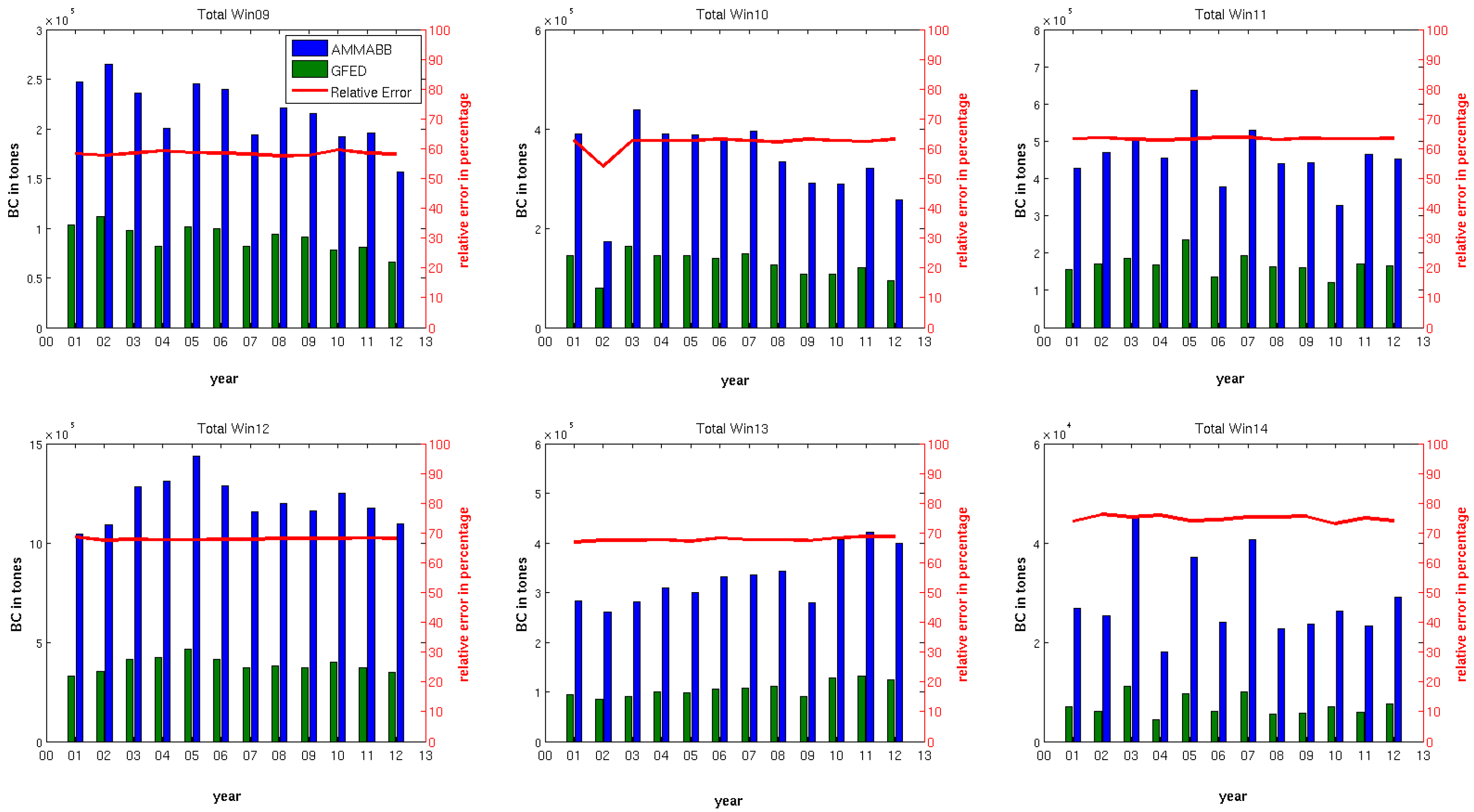
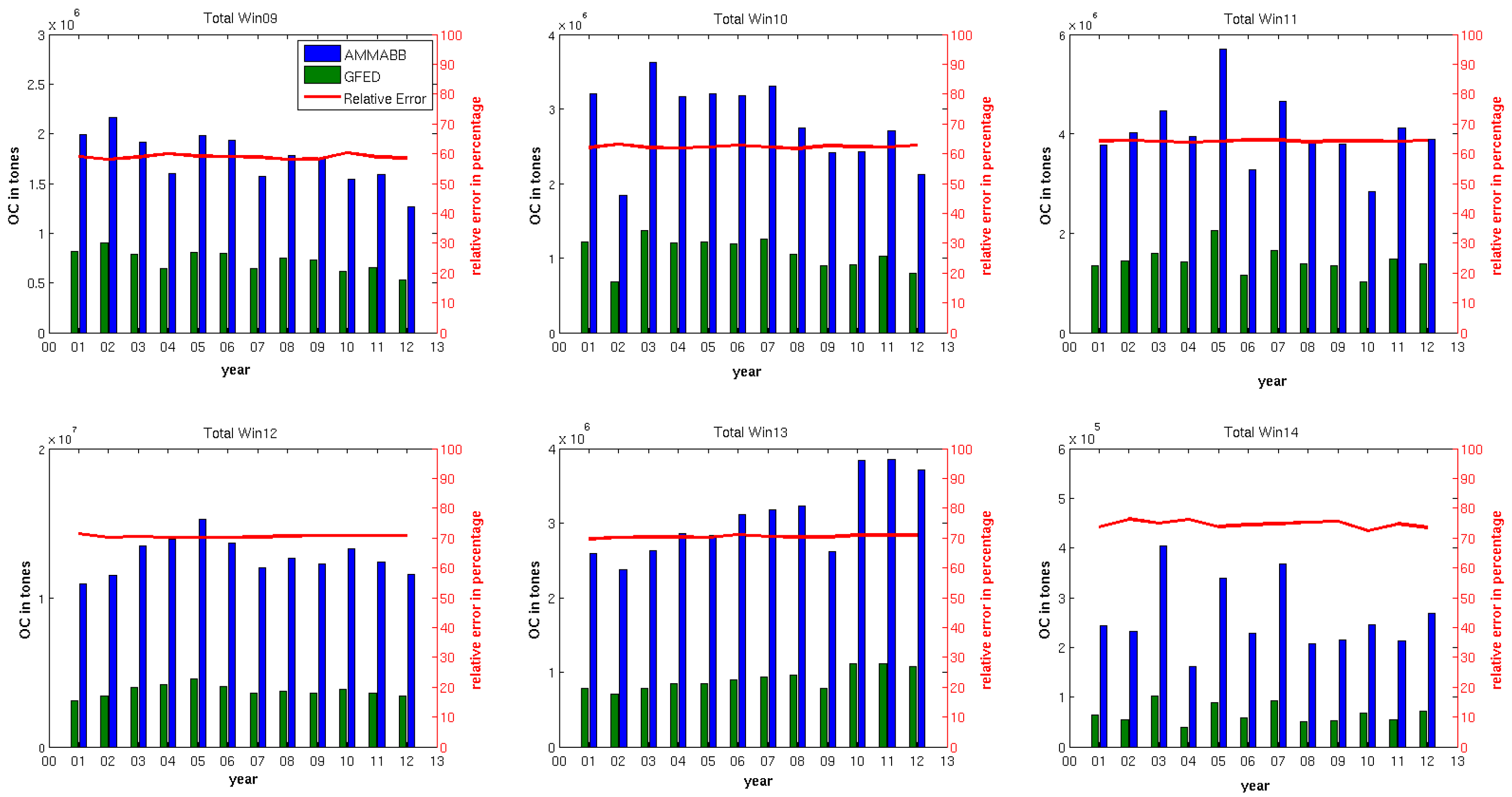
3.3. BC and OC Emissions Spatial Distribution

Using Equation (1), “AMMABB-like” and “GFED-like” emissions have been built using the vegetation parameters of AMMABB and GFED. Though several gases and particle emissions were calculated, we present here only the results for BC and OC. BC emissions spatial distribution for “AMMABB-like” (Figure 4a,e,i,m,q,u) and “GFED-like” (Figure 4b,f,j,n,r,v), their spatial differences (Figure 4c,g,k,o,s,w), and relative gaps (Figure 4d,h,l,p,t,x) revealed that important differences can be observed. These relative gaps are generally well above 60% in most parts of Africa, highlighting that “AMMABB-like” is well above “GFED-like.” Only a few areas have negative relative gaps of about 20%, underlining slightly higher “GFED-like” BC emissions associated with the fire season occurring during the boreal winter and summer seasons, which are associated with intense BB occurring in the northern and southern hemispheres of Africa, respectively. Similar patterns are also observed for OC (not shown here). “AMMABB-like” and “GFED4-like” time series of BC (Figure 5) and OC (Figure 6) emissions reveal important differences associated with relative gaps varying from 60% (northern hemisphere) to 75% (southern hemisphere). For both BC and OC, there is a slight inter-annual variability; the highest emissions are found over window 12 (central part of Africa) and lowest over window 14 (Madagascar Island). Since spatial differences are not uniform in all GLC vegetation classes and some vegetation classes may have a greater impact on total emissions than others, it is appropriate to investigate the contribution of each vegetation class to total emissions in the BC and OC cases.

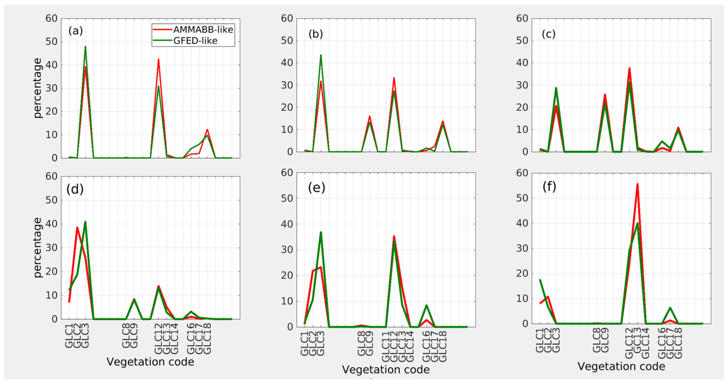
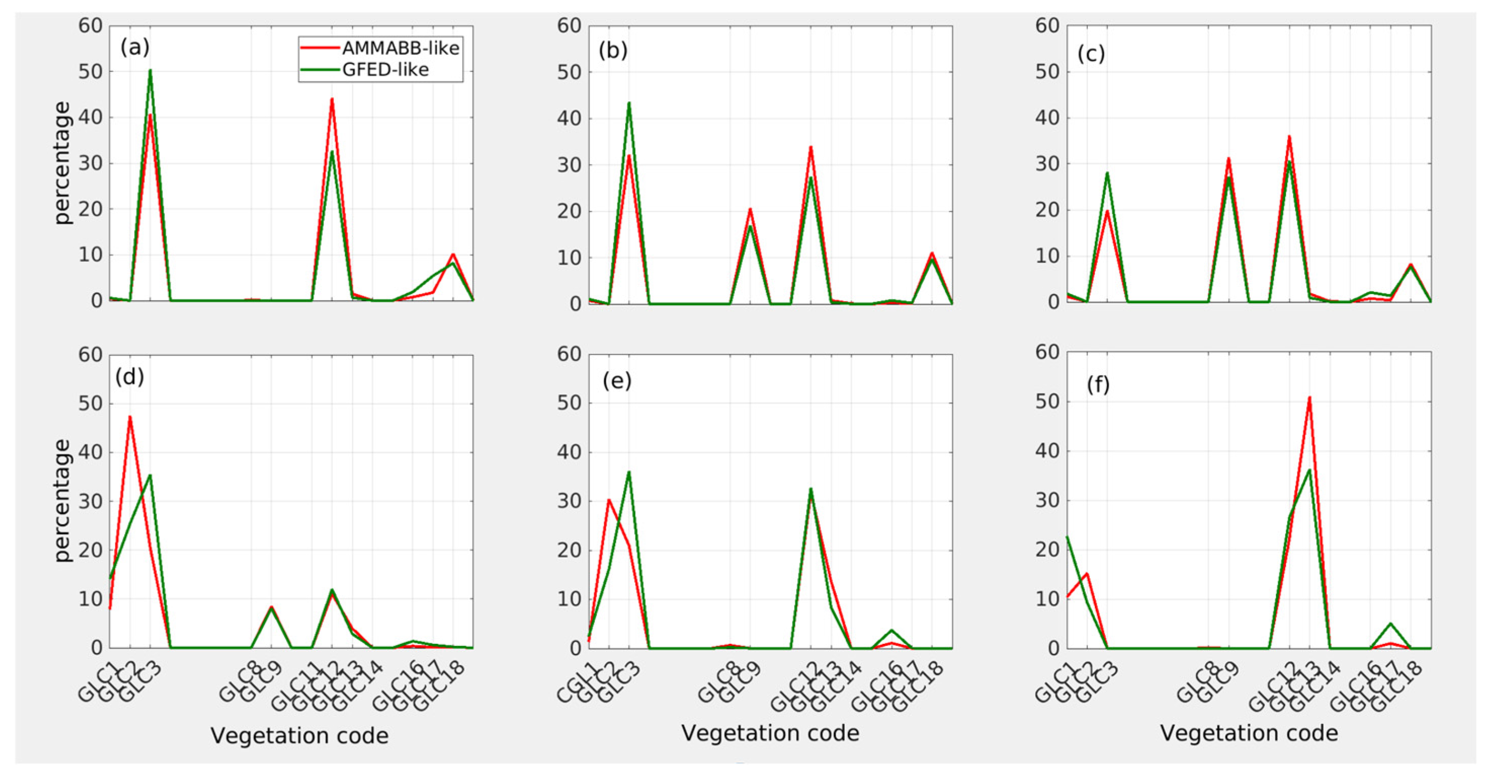
3.4. Vegetation Contribution to BC and OC Emissions

Since total BC and OC emissions are the sum of all vegetation classes, we determined the mean percentage of each vegetation class to the total emission. This mean proportion of the different vegetation classes represents its contribution to total BC and OC emissions and is presented in Figure 7 and Figure 8, respectively. We assumed that a contribution is significant when it is higher than or equal to 10%. Results show that depending on the emission inventories (“AMMABB-like” or “GFED4-like”) used, vegetation contributions to total BC and OC emissions are not the same. From Figure 7 and Figure 8, the highest contributors to the total BC and OC emissions are “AMMABB-like” and “GFED4-like” GLC3 (48% and 39%, respectively), GLC12 (42% and 31%, respectively), and GLC18 (12% and 10%, respectively) over West Africa (Win09). These main contributors are GLC3 (42% and 31%), GLC9 (18% and 14%), GLC12 (32% and 28%), and GLC18 (13% and 12%) over the north-central part of Africa (Win10) for “AMMABB-like” and “GFED4-like” BC and OC emissions. GLC3 (29% and 20%), GLC9 (26% and 22%), GLC12 (38% and 30%), and GLC18 (11% and 10%) are the main contributors to “AMMABB-like” and “GFED4-like” emissions over eastern Africa (Win 11). GLC1 (10% and 14%), GLC2 (38% and 19%), GL3 (28% and 40%), and GL12 (14% and 14%) are the main contributors over the central part of Africa (Win12) to “AMMABB-like” and “GFED4-like” emissions. Vegetation classes GLC2 (22% and 10%), GLC3 (37% and 24%), GLC12 (36% and 35%), and GLC13 (20% and 10%) were the major contributors to “AMMABB-like” and “GFED4-like” emissions over southern Africa (Win 13). GLC1 (9.8% and 18%), GLC2 (10% and 7%), GLC12 (30% and 25%), and GLC13 (55% and 40%) have been identified as the major contributors to the “AMMABB-like” and “GFED4-like” emissions over Madagascar (Win14). It can be noticed that GLC3 (Tree Cover, broadleaved, deciduous, open) and GLC12 (Shrub Cover, closed-open, deciduous) are the vegetation types present in all the African sub-regions considered in this work. Overall, GLC3 (Tree Cover, broadleaved, deciduous, open), GLC12 (Shrub Cover, closed-open, deciduous), GLC13 (Herbaceous Cover, closed-open), and GLC18 (Mosaic: Cropland/Shrub or Grass Cover) are the main contributors to the total BC and OC emissions from BB in Africa. In addition, the mean factors between the “AMMABB-like” and “GFED4-like” emissions are reported in Table 2. These ratios vary between 2.4 and 3.9, depending on the sub-region. The highest ratios are found in the southern hemisphere of Africa, with values higher than 3.

4. Discussion

Fuel availability plays a major role in fire sustainability, intensity [54,55], and spread and impacts atmospheric emissions [56]. In this work, we investigated the differences between the two “bottom-up” inventories AMMABB and GFED while focusing on the role of vegetation parameters, such as BD and BE, on total emission. In Africa, where savanna burning is a traditional practice for agriculture, hunting, and livestock, fires are usually used as a management tool. BE shows relatively little variability [57,58], while BD varies greatly on monthly timescales, depending on the season, time since fire, and grazing rates [59,60]. This may explain the differences between BEBDAMMABB and BEBDGFED, though close BE is used in the two inventories. Also, African savannas are split into wet and dry savannas following a threshold of annual precipitation of 900 mm year−1 [45,61], and BD consists of surface fuels (like grass and litter from trees) since it represents key fuel for fires [62,63,64].
However, depending on the annual precipitation amount, BD may be influenced both by rainfall of the previous years and the time since the last fire [65]. Indeed, the BD of savannas receiving more than 800 mm year−1 is considered less dependent on previous year rainfall (high BD) than those receiving less than 800 mm year−1 [46,64,66]. This suggests that uncertainties and gaps in African BB emissions inventories are likely to be attributed to the BD parameters considered in the existing bottom-up inventories. Comparing BC between “AMMABB-like” and “GFED4-like” emissions (Figure 4) reveals important differences, associated with relative gaps varying from 60% (northern hemisphere) to 75% (southern hemisphere). Similar spatial differences are also notable when considering the OC emissions (Figure A1). This is in agreement with previous studies using GFEDv2, GFEDv3, and AMMABB inventories [28,32]. The vegetation classes GLC3, GLC12, GLC13, and GLC18 are the main contributors to BC and OC emissions. This suggests that a better assessment or agreement between the existing emission inventories using a “bottom-up” approach, focusing on BD and BE of the GLC3 (Tree Cover Broadleaved, Deciduous Open), GLC12 (Shrub Cover, Closed-Open, Deciduous), GLC13 (Herbaceous Cover, Closed-Open), and GLC18 (Mosaic: Cropland/Shrub or Grass Cover), will help reduce the large “gaps” between the BB emission inventories built for Africa. Since BE and BD govern fuel consumption (FC) used in fire emissions models, a better assessment of BE and BD will help improve and validate these models [59]. Only a few measurements of FC exist for Africa despite the continent being prone to biomass fires and different types of savannas. With the growing use of the FRP, it is possible to retrieve FC by reverse calculation of the amount of combusted fuel required to produce the measured energy. Thus, this methodology has been applied at continental [67,68] and global [69] scales despite the fact that the FRP-derived FC has been found to be typically lower than those used in “bottom-up” methodologies such as GFED [67,68,69]. Moreover, differences have been reported in the agreement between FRP-derived FC and GFED estimates across the southern and northern hemispheres of Africa [70]. This work highlights that BEBD (or FC) used in AMMABB is higher than those used in GFED. This underlines the need for more in situ measurements of FC, at least on the main vegetation classes (GLC3, GLC12, GLC13, and GLC18) in the two hemispheres of Africa to reduce BB emission inventory uncertainties.

5. Conclusions

This work, using a “bottom-up” methodology, focused on explaining the 2.4-fold difference between the AMMABB and GFED emissions inventories. This discrepancy was related to various hypotheses, including methodology, fire product, EF, vegetation maps, BE, and BD, as the original inventories used different fire products (MODIS for GFED and L3JRC for the AMMABB), as well as differing EF, methodologies, and vegetation parameters. In this study, we used the same fire product (MODIS), the same EF, and the same methodology, but different burning efficiency and biomass density to reconstruct BB emissions in both “AMMABB-like” and “GFED-like” scenarios and to study the impact of vegetation parameters. We found that although the BE was similar in both inventories, BD exhibited important differences, leading to significant relative gaps in the BEBD (also known as FC). Specifically, we observed positive gaps over the Sahel and southern part of Africa (higher than 60%) and negative gaps over central Africa and the Horn of Africa (more than −70%). In addition, the relative gaps in vegetation class parameters vary between 44% for GLC 1 (Tree Cover Broadleaved Evergreen) to 85.12% for GLC 14 (Sparse Herbaceous/Sparse Shrub Cover). Finally, GLC3 (Tree Cover, broadleaved, deciduous, open), GLC12 (Shrub Cover, closed-open, deciduous), GLC13 (Herbaceous Cover, closed-open), and GLC18 (Mosaic: Cropland/Shrub or Grass Cover) are the main vegetation classes frequently burned and mostly contributing to the total emissions in Africa. Mean factors between the “AMMABB-like” and “GFED4-like” emissions ranged from 2.4 to 3.9, with higher values observed in the southern hemisphere. Therefore, these vegetation parameters play a crucial role in the various ranges and uncertainties found between BB inventories in Africa.
Thus, a more accurate assessment or improved agreement between the existing emission inventories, using a “bottom-up” approach focusing on BDBE (FC), supported by field measurements and distinguished between the northern and southern hemispheres of the main vegetation classes, would help reduce the large gaps observed between the BB emission inventories developed for Africa.

Author Contributions

Conceptualization, T.E.N. and C.L.; methodology, T.E.N., L.R. and C.L.; writing—original draft preparation, T.E.N. and C.L.; writing—review and editing, T.E.N., L.R., C.L. and A.B.N. All authors have read and agreed to the published version of the manuscript.

Funding

This research has been supported by the EU project (FP7/2007-2013) DACCIWA (Dynamics-aerosol-chemistry-cloud interactions in West Africa) under grant agreement no. 603502.

Institutional Review Board Statement

Not applicable.

Informed Consent Statement

Not applicable.

Data Availability Statement

The original contributions presented in this study are included in the article. Further inquiries can be directed to the corresponding author(s).

Acknowledgments

The authors are grateful to Prof van der Werf Guido and his team for providing GFED vegetation data, which were used to perform the present work. We would also like to thank the JEAI PATI (Jeune Equipe Associée de l’IRD Physico-chimie ATmosphérique et Impacts) for their financial support to finalize this work.

Conflicts of Interest

The authors declare no conflicts of interest.

Appendix A

Figure A1. Spatial distribution of mean OC emissions (tons/cell) at spatial resolution of 0.25° × 0.25° in “AMMABB-like” (first column), “GFED-like” (second column), their differences (third column), their relative gaps (fourth column) over Win09 (ad), Win10 (eh), Win11 (il), Win12 (mp), Win13 (qt) and Win14 (ux) of the sub-Saharan Africa domains of the collection 5 MODIS burned areas data.
Atmosphere 16 00440 g0a1

References

  1. van der Werf, G.R.; Randerson, J.T.; Giglio, L.; Collatz, G.J.; Kasibhatla, P.S.; Arellano, A.F., Jr. Interannual variability in global biomass burning emissions from 1997 to 2004. Atmos. Chem. Phys. 2006, 6, 3423–3441. [Google Scholar] [CrossRef]
  2. Barbosa, P.M.; Stroppiana, D.; Grégoire, J.M.; Cardoso Pereira, J.M. An assessment of vegetation fire in Africa (1981–1991): Burned areas, burned biomass, and atmospheric emissions. Glob. Biogeochem. Cycles 1999, 13, 933–950. [Google Scholar] [CrossRef]
  3. Norgrove, L.; Hauser, S. Estimating the consequences of fire exclusion for food crop production, soil fertility, and fallow recovery in shifting cultivation landscapes in the humid tropics. Environ. Manag. 2015, 55, 536–549. [Google Scholar] [CrossRef] [PubMed]
  4. N’Dri, A.B.; Kone, A.W.; Loukou, S.K.; Barot, S.; Gignoux, J. Carbon and nutrient losses through biomass burning, and links with soil fertility and yam (Dioscorea alata) production. Exp. Agric. 2019, 55, 738–751. [Google Scholar] [CrossRef]
  5. Veraverbeke, S.; Rogers, B.M.; Goulden, M.L.; Jandt, R.R.; Miller, C.E.; Wiggins, E.B.; Randerson, J.T. Lightning as a major driver of recent large fire years in North American boreal forests. Nat. Clim. Chang. 2017, 7, 529–534. [Google Scholar] [CrossRef]
  6. Seiler, W.; Crutzen, P.J. Estimates of gross and net fluxes of carbon between the biosphere and the atmosphere from biomass burning. Clim. Chang. 1980, 2, 207–247. [Google Scholar] [CrossRef]
  7. Andreae, M.O.; Crutzen, P.J. Atmospheric aerosols: Biogeochemical sources and role in atmospheric chemistry. Science 1997, 276, 1052–1058. [Google Scholar] [CrossRef]
  8. Laris, P.; Koné, M.; Dembélé, F.; Rodrigue, C.M.; Yang, L.; Jacobs, R.; Laris, Q.; Camara, F. The pyrogeography of methane emissions from seasonal mosaic burning regimes in a West African landscape. Fire 2023, 6, 52. [Google Scholar] [CrossRef]
  9. Fan, H.; Yang, X.; Zhao, C.; Yang, Y.; Shen, Z. Spatiotemporal variation characteristics of global fires and their emissions. Atmos. Chem. Phys. 2023, 23, 7781–7798. [Google Scholar] [CrossRef]
  10. Andreae, M.O. Biomass burning in the tropics: Impact on environmental quality and global climate. Popul. Dev. Rev. 1990, 16, 268–291. [Google Scholar] [CrossRef]
  11. Tripathi, S.; Yadav, S.; Sharma, K. Air pollution from biomass burning in India. Environ. Res. Lett. 2024, 19, 073007. [Google Scholar] [CrossRef]
  12. Yadav, I.C.; Devi, N.L. Biomass burning, regional air quality, and climate change. Encycl. Environ. Health 2019, 2, 386–391. [Google Scholar]
  13. Andela, N.; Van Der Werf, G.R. Recent trends in African fires driven by cropland expansion and El Niño to La Niña transition. Nat. Clim. Change 2014, 4, 791–795. [Google Scholar] [CrossRef]
  14. Ramo, R.; Roteta, E.; Bistinas, I.; van Wees, D.; Bastarrika, A.; Chuvieco, E.; van der Werf, G.R. African burned area and fire carbon emissions are strongly impacted by small fires undetected by coarse resolution satellite data. Proc. Natl. Acad. Sci. USA 2021, 118, e2011160118. [Google Scholar] [CrossRef]
  15. Damoah, R.; Spichtinger, N.; Forster, C.; James, P.; Mattis, I.; Wandinger, U.; Beirle, S.; Wagner, T.; Stohl, A. Around the world in 17 days-hemispheric-scale transport of forest fire smoke from Russia in May 2003. Atmos. Chem. Phys. 2004, 4, 1311–1321. [Google Scholar] [CrossRef]
  16. Martins, L.D.; Hallak, R.; Alves, R.C.; de Almeida, D.S.; Squizzato, R.; Moreira, C.A.; Beal, A.; da Silva, I.; Rudke, A.; Martins, J.A.; et al. Long-range transport of aerosols from biomass burning over southeastern South America and their implications on air quality. Aerosol Air Qual. Res. 2018, 18, 1734–1745. [Google Scholar] [CrossRef]
  17. Nguyen, L.S.P.; Huang, H.Y.; Lei, T.L.; Bui, T.T.; Wang, S.H.; Chi, K.H.; Sheu, G.R.; Lee, C.T.; Ou-Yang, C.F.; Lin, N.H. Characterizing a landmark biomass-burning event and its implication for aging processes during long-range transport. Atmos. Environ. 2020, 241, 117766. [Google Scholar] [CrossRef]
  18. Su, M.; Shi, Y.; Yang, Y.; Guo, W. Impacts of different biomass burning emission inventories: Simulations of atmospheric CO2 concentrations based on GEOS-Chem. Sci. Total Environ. 2023, 876, 162825. [Google Scholar] [CrossRef] [PubMed]
  19. Hua, W.; Lou, S.; Huang, X.; Xue, L.; Ding, K.; Wang, Z.; Ding, A. Diagnosing uncertainties in global biomass burning emission inventories and their impact on modeled air pollutants. Atmos. Chem. Phys. 2024, 24, 6787–6807. [Google Scholar] [CrossRef]
  20. Michel, C.; Liousse, C.; Grégoire, J.M.; Tansey, K.; Carmichael, G.; Woo, J.H. Biomass burning emission inventory from burnt area data given by the SPOT-VEGETATION system in the frame of TRACE-P and ACE-Asia campaigns. J. Geophys. Res. Atmos. 2005, 110. [Google Scholar] [CrossRef]
  21. Generoso, S.; Bey, I.; Attié, J.L.; Bréon, F.M. A satellite-and model-based assessment of the 2003 Russian fires: Impact on the Arctic region. J. Geophys. Res. Atmos. 2007, 112. [Google Scholar] [CrossRef]
  22. Stroppiana, D.; Brivio, P.; Grégoire, J.M.; Liousse, C.; Guillaume, B.; Granier, C.; Mieville, A.; Chin, M.; Pétron, G. Comparison of global inventories of CO emissions from biomass burning derived from remotely sensed data. Atmos. Chem. Phys. 2010, 10, 12173–12189. [Google Scholar] [CrossRef]
  23. Nguyen, H.M.; Wooster, M.J. Advances in the estimation of high Spatio-temporal resolution pan-African top-down biomass burning emissions made using geostationary fire radiative power (FRP) and MAIAC aerosol optical depth (AOD) data. Remote Sens. Environ. 2020, 248, 111971. [Google Scholar] [CrossRef]
  24. Shi, Y.; Zang, S.; Matsunaga, T.; Yamaguchi, Y. A multi-year and high-resolution inventory of biomass burning emissions in tropical continents from 2001–2017 based on satellite observations. J. Clean. Prod. 2020, 270, 122511. [Google Scholar] [CrossRef]
  25. Ellicott, E.; Vermote, E.; Giglio, L.; Roberts, G. Estimating biomass consumed from fire using MODIS FRE. Geophys. Res. Lett. 2009, 36. [Google Scholar] [CrossRef]
  26. Soja, A.J.; Cofer, W.R.; Shugart, H.H.; Sukhinin, A.I.; Stackhouse, P.W., Jr.; McRae, D.J.; Conard, S.G. Estimating fire emissions and disparities in boreal Siberia (1998–2002). J. Geophys. Res. Atmos. 2004, 109. [Google Scholar] [CrossRef]
  27. Van Der Werf, G.R.; Randerson, J.T.; Collatz, G.J.; Giglio, L. Carbon emissions from fires in tropical and subtropical ecosystems. Glob. Change Biol. 2003, 9, 547–562. [Google Scholar] [CrossRef]
  28. Liousse, C.; Guillaume, B.; Grégoire, J.M.; Mallet, M.; Galy, C.; Pont, V.; Akpo, A.; Bedou, M.; Castéra, P.; Dungall, L.; et al. Updated African biomass burning emission inventories in the framework of the AMMA-IDAF program, with an evaluation of combustion aerosols. Atmos. Chem. Phys. 2010, 10, 9631–9646. [Google Scholar] [CrossRef]
  29. Randerson, J.; Van Der Werf, G.; Giglio, L.; Collatz, G.; Kasibhatla, P. Global Fire Emissions Database, Version 4.1 (GFEDv4); ORNL DAAC: Oak Ridge, TN, USA, 2018. [Google Scholar]
  30. Kaiser, J.; Heil, A.; Andreae, M.; Benedetti, A.; Chubarova, N.; Jones, L.; Morcrette, J.J.; Razinger, M.; Schultz, M.; Suttie, M.; et al. Biomass burning emissions estimated with a global fire assimilation system based on observed fire radiative power. Biogeosciences 2012, 9, 527–554. [Google Scholar] [CrossRef]
  31. Tansey, K.; Grégoire, J.M.; Defourny, P.; Leigh, R.; Pekel, J.F.; Van Bogaert, E.; Bartholomé, E. A new, global, multi-annual (2000–2007) burnt area product at 1 km resolution. Geophys. Res. Lett. 2008, 35. [Google Scholar] [CrossRef]
  32. Williams, A.; Jones, J.; Ma, L.; Pourkashanian, M. Pollutants from the combustion of solid biomass fuels. Prog. Energy Combust. Sci. 2012, 38, 113–137. [Google Scholar] [CrossRef]
  33. Johnson, B.T.; Haywood, J.M.; Langridge, J.M.; Darbyshire, E.; Morgan, W.T.; Szpek, K.; Brooke, J.K.; Marenco, F.; Coe, H.; Artaxo, P.; et al. Evaluation of biomass burning aerosols in the HadGEM3 climate model with observations from the SAMBBA field campaign. Atmos. Chem. Phys. 2016, 16, 14657–14685. [Google Scholar] [CrossRef]
  34. Mallet, M.; Solmon, F.; Nabat, P.; Elguindi, N.; Waquet, F.; Bouniol, D.; Sayer, A.M.; Meyer, K.; Roehrig, R.; Michou, M.; et al. Direct and semi-direct radiative forcing of biomass-burning aerosols over the southeast Atlantic (SEA) and its sensitivity to absorbing properties: A regional climate modeling study. Atmos. Chem. Phys. 2020, 20, 13191–13216. [Google Scholar] [CrossRef]
  35. Zhong, Q.; Schutgens, N.; van der Werf, G.R.; Van Noije, T.; Bauer, S.E.; Tsigaridis, K.; Mielonen, T.; Checa-Garcia, R.; Neubauer, D.; Kipling, Z.; et al. Using modelled relationships and satellite observations to attribute modelled aerosol biases over biomass burning regions. Nat. Commun. 2022, 13, 5914. [Google Scholar] [CrossRef] [PubMed]
  36. Giglio, L.; Csiszar, I.; Justice, C.O. Global distribution and seasonality of active fires as observed with the Terra and Aqua Moderate Resolution Imaging Spectroradiometer (MODIS) sensors. J. Geophys. Res. Biogeosci. 2006, 111. [Google Scholar] [CrossRef]
  37. Giglio, L.; Randerson, J.; Van der Werf, G.; Kasibhatla, P.; Collatz, G.; Morton, D.; DeFries, R. Assessing variability and long-term trends in burned area by merging multiple satellite fire products. Biogeosciences 2010, 7, 1171–1186. [Google Scholar] [CrossRef]
  38. Potter, C.S.; Randerson, J.T.; Field, C.B.; Matson, P.A.; Vitousek, P.M.; Mooney, H.A.; Klooster, S.A. Terrestrial ecosystem production: A process model based on global satellite and surface data. Glob. Biogeochem. Cycles 1993, 7, 811–841. [Google Scholar] [CrossRef]
  39. Friedl, M.A.; McIver, D.K.; Hodges, J.C.; Zhang, X.Y.; Muchoney, D.; Strahler, A.H.; Woodcock, C.E.; Gopal, S.; Schneider, A.; Cooper, A.; et al. Global land cover mapping from MODIS: Algorithms and early results. Remote Sens. Environ. 2002, 83, 287–302. [Google Scholar] [CrossRef]
  40. Andreae, M.O.; Merlet, P. Emission of trace gases and aerosols from biomass burning. Glob. Biogeochem. Cycles 2001, 15, 955–966. [Google Scholar] [CrossRef]
  41. Liousse, C.; Andreae, M.O.; Artaxo, P.; Barbosa, P.; Cachier, H.; Grégoire, J.; Hobbs, P.; Lavoué, D.; Mouillot, F.; Penner, J.; et al. Deriving global quantitative estimates for spatial and temporal distributions of biomass burning emissions. In Emissions of Atmospheric Trace Compounds; Springer: Berlin/Heidelberg, Germany, 2004; pp. 71–113. [Google Scholar]
  42. Bian, H.; Chin, M.; Kawa, S.; Duncan, B.; Arellano, A.; Kasibhatla, P. Sensitivity of global CO simulations to uncertainties in biomass burning sources. J. Geophys. Res. Atmos. 2007, 112. [Google Scholar] [CrossRef]
  43. Carter, T.S.; Heald, C.L.; Jimenez, J.L.; Campuzano-Jost, P.; Kondo, Y.; Moteki, N.; Schwarz, J.P.; Wiedinmyer, C.; Darmenov, A.S.; da Silva, A.M.; et al. How emissions uncertainty influences the distribution and radiative impacts of smoke from fires in North America. Atmos. Chem. Phys. Discuss. 2019, 2019, 1–50. [Google Scholar] [CrossRef]
  44. Ramnarine, E.; Kodros, J.K.; Hodshire, A.L.; Lonsdale, C.R.; Alvarado, M.J.; Pierce, J.R. Effectsof near-source coagulation of biomass burning aerosols on global predictions of aerosol size distributions and implications for aerosol radiative effects. Atmos. Chem. Phys. 2019, 19, 6561–6577. [Google Scholar] [CrossRef]
  45. Menaut, J.C.; Abbadie, L.; Lavenu, F.; Loudjani, P.; Podaire, A. Biomass Burning in West African Savannas; Massachusetts Inst. of Tech. Press: Cambridge, MA, USA, 1991; pp. 133–142. [Google Scholar]
  46. N’Datchoh, E.; Konaré, A.; Diedhiou, A.; Diawara, A.; Quansah, E.; Assamoi, P. Effects of climate variability on savannah fire regimes in West Africa. Earth Syst. Dyn. 2015, 6, 161–174. [Google Scholar] [CrossRef]
  47. Soro, T.D.; Koné, M.; N’Dri, A.B.; N’Datchoh, E.T. Identified main fire hotspots and seasons in Cote d’lvoire (West Africa) using MODIS fire data. S. Afr. J. Sci. 2021, 117, 1–13. [Google Scholar] [CrossRef]
  48. Mayaux, P.; Eva, H.; Gallego, J.; Strahler, A.H.; Herold, M.; Agrawal, S.; Naumov, S.; De Miranda, E.E.; Di Bella, C.M.; Ordoyne, C.; et al. Validation of the global land cover 2000 map. IEEE Trans. Geosci. Remote Sens. 2006, 44, 1728–1739. [Google Scholar] [CrossRef]
  49. Roy, D.P.; Boschetti, L.; Justice, C.; Ju, J. The collection 5 MODIS burned area product—Global evaluation by comparison with the MODIS active fire product. Remote Sens. Environ. 2008, 112, 3690–3707. [Google Scholar] [CrossRef]
  50. Pereira, J.; Chuvieco, E.; Beaudoin, A.; Desbois, N. Remote Sensing of Burned Areas: A Review. A Review of Remote Sensing Methods for the Study of Large Wildland Fires; Departamento de Geografa, Universidad de Alcal: Alcalá de Henares, Spain, 1997; pp. 127–184. [Google Scholar]
  51. Roy, D.P. Multi-temporal active-fire based burn scar detection algorithm. Int. J. Remote Sens. 1999, 20, 1031–1038. [Google Scholar] [CrossRef]
  52. Boschetti, L.; Roy, D.P.; Justice, C.O.; Humber, M.L. MODIS–Landsat fusion for large area 30 m burned area mapping. Remote Sens. Environ. 2015, 161, 27–42. [Google Scholar] [CrossRef]
  53. Bartholome, E.; Belward, A.S. GLC2000: A new approach to global land cover mapping from Earth observation data. Int. J. Remote Sens. 2005, 26, 1959–1977. [Google Scholar] [CrossRef]
  54. Thaxton, J.M.; Platt, W.J. Small-scale fuel variation alters fire intensity and shrub abundance in a pine savanna. Ecology 2006, 87, 1331–1337. [Google Scholar] [CrossRef]
  55. dos Santos, A.C.; da Rocha Montenegro, S.; Schmidt, I.B. Fire season and fuel load predict fire behavior in open savannas in Northern Cerrado. Biodiversidade Bras. 2019, 9, 91. [Google Scholar]
  56. Di Giuseppe, F.; Benedetti, A.; Coughlan, R.; Vitolo, C.; Vuckovic, M. A global bottom-up approach to estimate fuel consumed by fires using above ground biomass observations. Geophys. Res. Lett. 2021, 48, e2021GL095452. [Google Scholar] [CrossRef]
  57. Savadogo, P.; Zida, D.; Sawadogo, L.; Tiveau, D.; Tigabu, M.; Odén, P.C. Fuel and fire characteristics in savanna–woodland of West Africa in relation to grazing and dominant grass type. Int. J. Wildland Fire 2007, 16, 531–539. [Google Scholar] [CrossRef]
  58. N’Dri, A.B.; Konan, L.N. Does the date of burning affect carbon and nutrient losses in a humid savanna of West Africa. Environ. Nat. Resour. Res. 2018, 8, 102. [Google Scholar]
  59. van Leeuwen, T.T.; van der Werf, G.R.; Hoffmann, A.A.; Detmers, R.G.; Rücker, G.; French, N.H.; Archibald, S.; Carvalho, J., Jr.; Cook, G.D.; de Groot, W.J.; et al. Biomass burning fuel consumption rates: A field measurement database. Biogeosciences 2014, 11, 7305–7329. [Google Scholar] [CrossRef]
  60. Laris, P.; Koné, M.; Dembélé, F.; Rodrigue, C.M.; Yang, L.; Jacobs, R.; Laris, Q. Methane gas emissions from savanna fires: What analysis of local burning regimes in a working West African landscape tell us. Biogeosciences 2021, 18, 6229–6244. [Google Scholar] [CrossRef]
  61. Sankaran, M.; Hanan, N.P.; Scholes, R.J.; Ratnam, J.; Augustine, D.J.; Cade, B.S.; Gignoux, J.; Higgins, S.I.; Le Roux, X.; Ludwig, F.; et al. Determinants of woody cover in African savannas. Nature 2005, 438, 846–849. [Google Scholar] [CrossRef]
  62. Balch, J.K.; Bradley, B.A.; D’Antonio, C.M.; Gómez-Dans, J. Introduced annual grass increases regional fire activity across the arid western USA (1980–2009). Glob. Change Biol. 2013, 19, 173–183. [Google Scholar] [CrossRef]
  63. Cardoso, A.W.; Archibald, S.; Bond, W.J.; Coetsee, C.; Forrest, M.; Govender, N.; Lehmann, D.; Makaga, L.; Mpanza, N.; Ndong, J.E.; et al. Quantifying the environmental limits to fire spread in grassy ecosystems. Proc. Natl. Acad. Sci. USA 2022, 119, e2110364119. [Google Scholar] [CrossRef]
  64. N’Dri, A.B.; Kpré, A.J.N.; Doumbia, A. Managing fires in a woody encroachment context: Fine fuel load does not change across fire seasons in a Guinean savanna (West Africa). J. Environ. Manag. 2024, 371, 123236. [Google Scholar] [CrossRef]
  65. Gill, A.M.; Allan, G. Large fires, fire effects and the fire-regime concept. Int. J. Wildland Fire 2008, 17, 688–695. [Google Scholar] [CrossRef]
  66. Mbow, C.; Nielsen, T.T.; Rasmussen, K. Savanna fires in east-central Senegal: Distribution patterns, resource management and perceptions. Hum. Ecol. 2000, 28, 561–583. [Google Scholar] [CrossRef]
  67. Andela, N.; Van Der Werf, G.R.; Kaiser, J.W.; Van Leeuwen, T.T.; Wooster, M.J.; Lehmann, C.E. Biomass burning fuel consumption dynamics in the tropics and subtropics assessed from satellite. Biogeosciences 2016, 13, 3717–3734. [Google Scholar] [CrossRef]
  68. Roberts, G.; Wooster, M.J.; Xu, W.; He, J. Fire activity and fuel consumption dynamics in sub-Saharan Africa. Remote Sens. 2018, 10, 1591. [Google Scholar] [CrossRef]
  69. Mota, B.; Wooster, M.J. A new top-down approach for directly estimating biomass burning emissions and fuel consumption rates and totals from geostationary satellite fire radiative power (FRP). Remote Sens. Environ. 2018, 206, 45–62. [Google Scholar] [CrossRef]
  70. Roberts, G.; Wooster, M.; Freeborn, P.; Xu, W. Integration of geostationary FRP and polar-orbiter burned area datasets for an enhanced biomass burning inventory. Remote Sens. Environ. 2011, 115, 2047–2061. [Google Scholar] [CrossRef]
Figure 1. The GLC2000 map and 6 African domain windows considered for the BB emission inventories gaps (source https://forobs.jrc.ec.europa.eu/glc2000/data, accessed on 5 April 2025).
Atmosphere 16 00440 g001
Figure 2. Comparison of the spatial distribution of (a) BEGFED, (b) BEAMMABB, (c) BE relative gaps (d), BDGFED, (e) BDAMMABB, (f) BD relative gaps, (g) BEBDGFED, (h) BEBDAMMABB, and (i) BEBD relative gaps from GFED4 and AMMABB in percentage.
Atmosphere 16 00440 g002
Figure 3. Yearly burned vegetation variability over sub-Saharan Africa between 2001 and 2012, for the relevant GLC classes (GLC1 (Tr. cov. broad. ever.), GLC2 (Tr. cov. Broad. Decid. closed), GLC3 (Tr. cov. Broad. Decid. open), GLC8 (Tr. Cov. Reg. Flood. Sal. Wat), GLC9 (Mos. Tr. Cov./Oth. Nat. Veget.), GLC12 (Shr. Cov. Closed-open, decid.), GLC13 (Herb. Cov. Closed-open), GLC14 (Spar. Herb./spar. Shr. Cov), GLC16 (Cult. And man. areas), GLC17 (Mos. Crop./Tr. Cov./Oth. Nat.Veget.) and GLC18 (Mos. Crop./Shr. Grass Cov.)) and MODIS windows (a) Win09; (b) Win 10; (c) Win 11; (d) Win 12; (e) Win 13 and (f) Win 14 as defined in Figure 1. Subplots use different scales for clarity.
Atmosphere 16 00440 g003
Figure 4. Spatial distribution of mean BC emissions (tons/cell) at spatial resolution of 0.25° × 0.25° in “AMMABB-like” (first column), “GFED-like” (second column), their differences (third column), their relative gaps (fourth column) over Win09 (ad), Win10 (eh), Win11 (il), Win12 (mp), Win13 (qt) and Win14 (ux) of the sub-Saharan Africa domains of the collection 5 MODIS burned areas data.
Atmosphere 16 00440 g004
Figure 5. BC emissions (scales different for each sub-figure) and the corresponding relative gaps (red line) for each of the sub-Saharan Africa domains of the collection 5 MODIS burned areas.
Atmosphere 16 00440 g005
Figure 6. OC emissions (scales different for each sub-figure) and the corresponding relative gaps (red line) for each of the sub-Saharan Africa domains of the collection 5 MODIS burned areas.
Atmosphere 16 00440 g006
Figure 7. Vegetation classes contribution to BC emissions for each sub-Saharan Africa domain of the collection 5 MODIS burned areas. (a) Win09, (b) Win10, (c) Win11, (d) Win12, (e) Win13 and (f) Win14 as shown in Figure 1.
Atmosphere 16 00440 g007
Figure 8. Vegetation classes contribution to OC emissions for each sub-Saharan Africa domain of the collection 5 MODIS burned areas. (a) Win09, (b) Win10, (c) Win11, (d) Win12, (e) Win13, and (f) Win14 as shown in Figure 1.
Atmosphere 16 00440 g008
Table 1. BE, BD, and the product of BD and BE values used in AMMABB and corresponding ratio GFED and their emissions relative gaps over the MODIS windows considered in this work.
AMMABBGFEDRatios (AMMABB/GFED)BDBE Relative DifferenceMean Burned Vegetation
GLC NameGLC CodeBEBD (kg/m2)BDBE (kg/m2)BEBD (kg/m2)BDBE (kg/m2)BE RatioBD Ratio BDBE Ratio (%)Win09 (%)Win10 (%)Win11 (%)Win12 (%)Win13 (%)Win14 (%)
Tr. cov. broad. ever.10.2523.355.8370.3968.2163.2530.6312.8421.79544.270.11 ± 0.040.30 ± 0.070.43 ± 0.123.24 ± 0.540.39 ± 0.162.39 ± 0.68
Tr. cov. Broad. Decid. closed20.25205.0000.7151.0910.7800.35018.3356.41284.40.000.000.02 ± 0.0118.04 ± 1.168.84 ± 0.924.42 ± 0/97
Tr. cov. Broad. Decid. open30.43.31.3200.2080.8730.6721.9233.7801.96549.0834.21 ± 2.4328.54 ± 0.8415.91 ± 0.9037.16 ± 0.7728.04 ± 1.370.00
Tr. cov. Needle-leav. Ever.40.2536.79.175-------0.000.000.000.000.000.00
Tr. Cov. Needle-leav. Decid.50.2518.94.725-------0.000.000.000.000.000.00
Tr. Cov. Mixed. Leaf typ.60.25143.5000.695--0.360---0.000.000.000.000.000.00
Tr. Cov. Regul. Flood. Fresh wat. (brackish)70.25276.7500.29820.210 0.83991.3362.1591000.000.000.000.000.000.00
Tr. Cov. Reg. Flood. Sal. Wat.80.6148.4000.6135.4320.9140.9792.5779.18989.120.03 ± 0.010.000.000.000.20 ± 0.060.06 ± 0.02
Mos. Tr. Cov./Oth. Nat. Veget.90.35103.5000.6741.1491.0850.5198.7003.22669.000.01 ± 0.0038.16 ± 1.3210.47 ± 1.804.55 ± 1.430.03 ± 0.010.00
Tr. cov. burnt10----------0.000.000.000.000.000.00
Shr. Cov. Closed-open, ever.110.91.251.1250.8180.501-1.1002.494--0.000.000.000.000.000.00
Shr. Cov. Closed-open, decid.120.43.31.3200.7990.5010.4010.5016.5853.29569.6238.93 ± 0.8232.16 ± 1.7037.67 ± 1.6722.16 ± 0.4833.95 ± 1.2431.67 ± 2.9
Herb. Cov. Closed-open130.91.4251.2820.8500.2720.2321.0595.2305.52181.900.58 ± 0.340.75 ± 0.241.69 ± 0.516.99 ± 0.5210.86 ± 1.3158.57 ± 2.75
Spar. Herb./spar. Shr. Cov140.60.90.5400.9060.0880.0800.66210.2276.77085.180.07 ± 0.090.12 ± 0.110.40 ± 0.170.04 ± 0.030.07 ± 0.070.00
Reg. Flood. Shr./Heb. Cov.150.259.552.3870.3170.9210.7010.78910.3703.40570.630.02 ± 0.011.25 ± 0.172.42 ± 0.620.49 ± 0.052.48 ± 0.540.00
Cult. And man. areas160.60.400.2640.7800.3380.2640.7691.3011.0010.004.77 ± 1.193.03 ± 0.559.83 ± 0.766.35 ± 0.4814.70 ± 1.260.01 ± 0.007
Mos. Crop./Tr. Cov./Oth. Nat.Veget.170.35103.5000.52248.3091.1080.6700.2073.15868.343.35 ± 0.830.22 ± 0.061.00 ± 0.260.38 ± 0.150.06 ± 0.022.81 ± 0.81
Mos. Crop./Shr. Grass Cov.180.7510.7500.8500.2900.2460.8823.4453.05067.217.70 ± 1.6625.28 ± 1.3319.96 ± 1.160.38 ± 0.120.000.00
Bare areas19-----0.055----0.01 ± 0.010.09 ± 0.100.17 ± 0.010.000.16 ± 0.100.00
Water bodies20-----0.504----0.19 ± 0.050.12 ± 0.030.04 ± 0.020.20 ± 0.030.08 ± 0.010.07 ± 0.02
Snow and Ice21----------0.000.000.000.000.000.00
Artf. Surf. And asso. areas22-----0.075----0.000.000.000.000.13 ± 0.040.00
Table 2. Mean BC and OC “AMMABB-like” and “GFED4-like” emissions mean for each African sub-region as indicated in Figure 1.
Win09Win10Win11Win12Win13Win14
Mean reatio AMMABB-like/GFED-LikeBCOCBCOCBCOCBCOCBCOCBCOC
2.4022.4312.6592.6502.7302.7943.1223.3923.1153.3933.9733.930
Disclaimer/Publisher’s Note: The statements, opinions and data contained in all publications are solely those of the individual author(s) and contributor(s) and not of MDPI and/or the editor(s). MDPI and/or the editor(s) disclaim responsibility for any injury to people or property resulting from any ideas, methods, instructions or products referred to in the content.

