Atmospheric Modeling for Wildfire Prediction

Abstract

Machine learning and artificial intelligence models have become popular for climate change prediction. Forested regions in California and Western Australia are increasingly facing intense wildfires, while other parts of the world face various climate-related challenges. To address these issues, machine learning and artificial intelligence models have been developed to predict wildfire risks and support mitigation strategies. Our study focuses on developing wildfire prediction models using one-class classification algorithms. These include Support Vector Machine, Isolation Forest, AutoEncoder, Variational AutoEncoder, Deep Support Vector Data Description, and Adversarially Learned Anomaly Detection. The models were validated through five-fold cross-validation to minimize bias in selecting training and testing data. The results showed that these one-class machine learning models outperformed two-class machine learning models based on the same ground truth data, achieving mean accuracy levels between 90% and 99%. Additionally, we employed Shapley values to identify the most significant features affecting the wildfire prediction models, contributing a novel perspective to wildfire prediction research. When analyzing models trained on the California dataset, seasonal maximum and mean dew point temperatures were critical factors. These insights can significantly improve wildfire mitigation strategies. Furthermore, we have made these models accessible and user-friendly by operationalizing them through a REST API using Python Flask 1.1.2 and developing a web-based tool.

1. Introduction

Wildfires have emerged as a critical global concern, annually destroying vast forested areas and significantly impacting the environment, economy, and public health. The urgency of this problem cannot be overstated. The natural causes of wildfires include lightning strikes, volcanic eruptions, dry climates, and dense vegetation. However, studies indicate that human activities—such as unattended campfires, discarded cigarettes, and intentional acts of arson—are responsible for nearly 85–90% of wildfire occurrences. This alarming trend underscores the need for continuous monitoring and, more importantly, predictive capabilities to forecast the likelihood of widespread and intense wildfires. Such foresight allows fire management authorities to take timely actions to mitigate damage.

Machine learning (ML) and artificial intelligence (AI) methods offer promising tools for developing predictive wildfire models [1]. For example, the European Centre for Medium-Range Weather Forecasts has developed the Probability of Fire (PoF) tool, which employs ML techniques to forecast fire occurrences globally with high resolution, up to ten days in advance [2]. Nevertheless, several challenges hinder the effectiveness of these models. These include technical limitations (such as specific technical limitations, e.g., computational power, data processing speed) and environmental complexities (such as specific environmental complexities, e.g., the influence of topography on fire spread), as well as the difficulty in identifying specific factors that contribute to wildfire ignition. Variations in atmospheric conditions—such as air temperature, relative humidity, wind speed and direction, and spatiotemporal dynamics—further complicate these predictions [3,4]. Another significant challenge is the infrequent and irregular occurrence of wildfires, which makes it difficult to acquire balanced datasets for training models that distinguish wildfire from non-wildfire events [5].

To address this issue, one-class classification approaches are explored. These methods are particularly effective for anomaly detection tasks where only positive class data are available, such as in predicting rare events or fraud detection [5,6]. Standard algorithms include one-class SVM, Isolation Forest, and Autoencoders. In contrast, two-class (binary) classification is designed for datasets with two labeled categories, aiming to differentiate between them—this is useful in applications like spam filtering or disease diagnosis [7]. While binary classification performs well for balanced datasets, one-class classification is better suited for scenarios with limited class variety, which influences the selection of appropriate models and evaluation metrics [5].

Despite the advancements in wildfire prediction models, few progress to deployment, limiting their practical applications. This study, however, aims to bridge this gap and make a significant contribution to the field. By integrating ML models into Application Programming Interfaces (APIs) to create user-friendly tools, we aim to enhance the utility of wildfire prediction systems. Our work is not just a study, but a potential game-changer in the field of wildfire prediction.

• A comparative evaluation of one-class classification algorithms and two-class models is conducted to determine their suitability for predicting wildfire risk using two fire incidence datasets.
• Shapley values [8] are used to interpret feature importance within one-class ML models, providing explainability and insights into the factors influencing wildfire predictions.
• A novel architecture for a web-based wildfire prediction tool is proposed, operationalizing the best-performing one-class ML model via a REST API.

The study focuses on California and Western Australia as contexts for wildfire probability prediction. California, a high-risk wildfire zone in the United States, recorded 4.2 million acres burned in a single year, resulting in 31 human fatalities [9]. Similarly, the 2019–2020 Australian wildfires devastated 17 million acres, causing the loss of three billion animals. New South Wales and the Australian Capital Territory accounted for 31.6 million acres burned, while Western Australia ranked second with approximately 5.4 million acres lost [10,11].

This work aims to assess the performance of one-class ML algorithms in predicting wildfire risk using historical fire data from California (2012–2016) and Western Australia (2000–2020). These regions were chosen due to their high incidence of wildfires and the availability of comprehensive historical data. By focusing on these regions, this study aims to provide insights into the efficacy of one-class models in overcoming the challenges of wildfire risk prediction and enhancing mitigation strategies.

The structure of this paper is organized as follows: Section 2 outlines the study’s background and details the one-class ML algorithms used in our experiments. Section 4 introduces the dataset employed for the case studies in California and Western Australia. Our proposed methodology is explained in Section 3, and Section 5 presents the corresponding results. The deployment process of the ML models is discussed in Section 6, followed by an evaluation of the web-based prototype in Section 7. Section 8 highlights potential threats to validity and the limitations. Section 9 summarizes our key findings in this study and suggests directions for future research.

2. Background

Defining a negative sample dataset for complex events such as wildfires presents significant challenges. Numerous non-fire data points could be incorrectly labeled without proper validation for a specific location, date, and time. This issue can be addressed using a one-class classification model, which establishes a class boundary based solely on positive data labels [1,6,12].

In one-class classification, the model assigns a data point as an inlier (•) if its probability exceeds the chosen threshold. Conversely, if the probability is below the threshold, the data point is classified as an outlier (?), as illustrated in Figure 1a. The selection of an accurate threshold is crucial to ensure the correct classification of inliers and outliers. Typically, the classification boundary in one-class learning is designed to accept most positive data labels while rejecting only a minimal number of outliers, as shown in Figure 1b. During training, the model relies exclusively on positive data labels, treating outliers as negative labels or non-fire events [5,6].

This approach has effectively tackled problems such as anomaly detection, outlier identification, and concept-based learning, particularly in cases where labeled negative samples are scarce or unreliable [7]. It provides a robust framework for learning from positive data while mitigating the risk of incorrectly labeling complex events like wildfires.

As previously mentioned, the model’s predicted probabilities and classification of inliers and outliers depend on the selected threshold value. If this threshold surpasses a specific level for a given prediction instance (p. 159, [10,13]), the instance is classified as a fire (inlier). The functionality of each one-class ML algorithm used in our experiments is outlined below.

Regarding our approach, the Support Vector Machine (SVM) is a supervised learning technique designed to analyze data and identify patterns for classification and regression problems [14]. The one-class variation of SVM (OCSVM) exists in two primary forms. The first, standard OCSVM, fits a minimal-volume hypersphere enclosing a predetermined fraction of training samples [15]. The second type constructs a decision boundary using a hyperplane in a transformed kernel space. In this method, data are mapped to a higher-dimensional space to evaluate whether a hyperplane can separate the classes, assuming that training samples belong to one class while non-training samples belong to another.

We employed the latter OCSVM approach to build the ML model for our experiments. This one-class OCSVM model identifies dense regions of standard data, while anomalies appear in low-density areas. New data instances are classified based on density estimates, distinguishing between normal and anomalous cases.

The Isolation Forest (IF) algorithm utilizes a binary tree structure, where each node randomly chooses a feature along with a splitting threshold [16]. This procedure continues until every node corresponds to a single instance. The method creates a collection of trees, in which anomalies, because of their uniqueness, are usually isolated more quickly in the tree construction process than clustered data points. Consequently, the average depth of samples throughout the ensemble has a direct impact on the anomaly score [16].

A comprehensive review of ML and AI techniques applied to wildfire prediction is presented in Table 1 [17], covering models based on Artificial Neural Networks (ANN), including those using Radial Basis Function ANNs [18]. In our study, we similarly utilized an AutoEncoder (AE), a type of multi-layer ANN designed for unsupervised learning. AE replicates input values at its output, thereby mapping high-dimensional data to a lower-dimensional representation [19]. The hidden layers encode the input in a way that reduces reconstruction error, ensuring that they capture the most relevant data patterns while filtering out noise. Anomalies are characterized by high reconstruction errors. Unlike AE, the Variational AutoEncoder (VAE) estimates the parameters of a probability distribution that models the data, which may enhance anomaly detection capabilities [19].

DeepSVDD [20] operates similarly to AE and VAE by jointly optimizing network parameters while minimizing the average distance between data points and the learned center of a hypersphere. Normal instances are mapped close to the center, whereas anomalies are positioned further away or outside the hypersphere [21]. In DeepSVDD, artificial neural networks (ANNs) function as one-class classifiers, rejecting any outlier instances. The network weights are learned from the training data and subsequently used to evaluate new instances. DeepSVDD [20] and ALAD [22] were chosen for our study due to their effectiveness in predictive modeling tasks.

Lastly, ALAD [22] is an anomaly detection method based on reconstruction, measuring how well a sample is regenerated by a Generative Adversarial Network (GAN). GANs are effective at modeling intricate, high-dimensional distributions found in real-world datasets, making them particularly suitable for anomaly detection. ALAD is based on bidirectional GANs, incorporating an encoder network that transforms input samples into a latent space representation. During training, the model learns an encoder that facilitates efficient mapping from data space to latent space, improving test-time performance. ALAD identifies anomalies by assessing the discrepancy between a sample and its reconstruction by the GAN—standard samples should be reconstructed accurately. In contrast, anomalous ones tend to have high reconstruction errors.

Our experiments used the OCSVM implementation from Python 3.8.3’s scikit-learn 0.24.1 package [23]. The remaining algorithms, including an alternative OCSVM implementation, were sourced from the Python PyOD package [24].

Table 1. Overview of one-class model types for anomaly detection.

One-Class Model Type	Description	Key Strengths	Limitations	Citations	Performance
Density based	Uses data density estimation with thresholds to distinguish data. Works well with large datasets. Common algorithms: Gaussian and Parzen models.	Effective with large datasets	Requires a large number of training samples	[25]	Effective for large datasets; accuracy depends on density estimation quality.
Boundary based	Defines a boundary using inliers; outliers fall outside the boundary. Works well with smaller datasets. Common algorithms: one-class SVM, Support Vector Data Description.	Works well with smaller datasets	Difficult to optimize boundaries	[26]	Performs well on smaller datasets; sensitive to boundary optimization.
Reconstruction based	Uses historical data to categorize outliers based on reconstruction error. Common algorithms: k-means, PCA, Autoencoder, Multi-layer Perceptron.	Utilizes historical data for anomaly detection	High training time for neural network-based approaches	[27,28,29,30]	High performance in learning training data; long training time.
Ensemble based	Uses ensemble learning techniques to improve classification performance. Common algorithms: one-class Random Forest, Isolation Forest.	Enhances classification performance with artificial outlier generation	Complex model structure	[16,25,31]	Improves classification accuracy; suitable for artificial outlier detection.
Clustering based	Reduces processing time by clustering feature space. Not tested due to limited data events.	Reduces processing time	Limited applicability with small datasets	[32]	Fast processing; performance depends on clustering quality and dataset size.

Table 1. Overview of one-class model types for anomaly detection.

One-Class Model Type	Description	Key Strengths	Limitations	Citations	Performance
Density based	Uses data density estimation with thresholds to distinguish data. Works well with large datasets. Common algorithms: Gaussian and Parzen models.	Effective with large datasets	Requires a large number of training samples	[25]	Effective for large datasets; accuracy depends on density estimation quality.
Boundary based	Defines a boundary using inliers; outliers fall outside the boundary. Works well with smaller datasets. Common algorithms: one-class SVM, Support Vector Data Description.	Works well with smaller datasets	Difficult to optimize boundaries	[26]	Performs well on smaller datasets; sensitive to boundary optimization.
Reconstruction based	Uses historical data to categorize outliers based on reconstruction error. Common algorithms: k-means, PCA, Autoencoder, Multi-layer Perceptron.	Utilizes historical data for anomaly detection	High training time for neural network-based approaches	[27,28,29,30]	High performance in learning training data; long training time.
Ensemble based	Uses ensemble learning techniques to improve classification performance. Common algorithms: one-class Random Forest, Isolation Forest.	Enhances classification performance with artificial outlier generation	Complex model structure	[16,25,31]	Improves classification accuracy; suitable for artificial outlier detection.
Clustering based	Reduces processing time by clustering feature space. Not tested due to limited data events.	Reduces processing time	Limited applicability with small datasets	[32]	Fast processing; performance depends on clustering quality and dataset size.

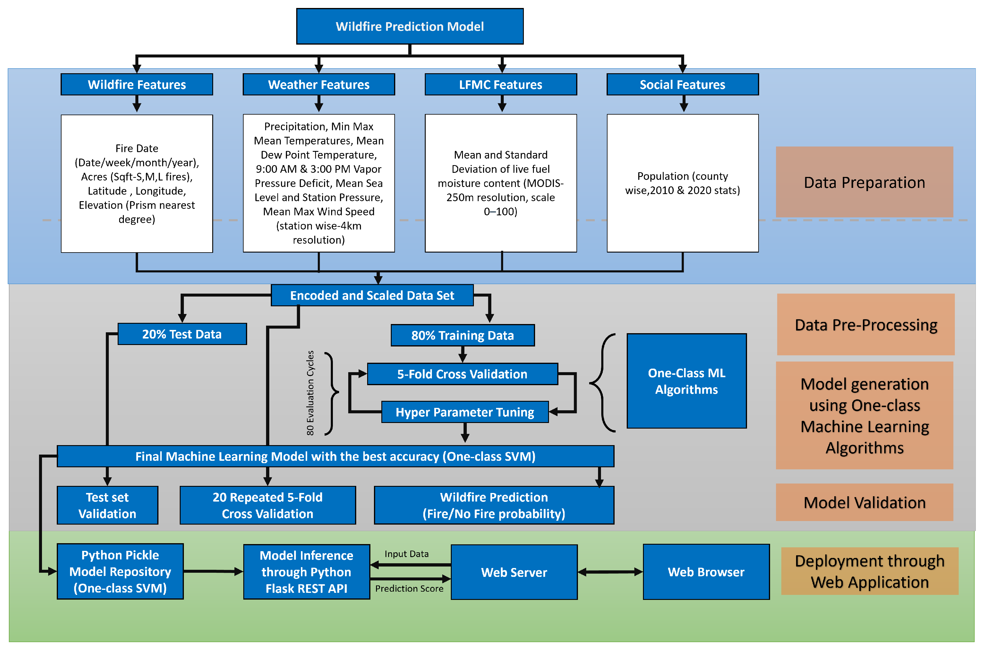
3. Methodology

As demonstrated in Figure 2, developing a decision support system for wildfire prediction involves several steps, including data preparation, processing, modeling, the validation of ML models, and the potential for deployment of ML models.

The input data are meticulously categorized into four groups: wildfire characteristics, weather-related attributes, Live Fuel Moisture Content (LFMC) indicators, and social factors. The dataset undergoes comprehensive pre-processing, including encoding and scaling, to ensure the robustness of the ML models using one-class classification. A detailed explanation of these thorough pre-processing steps follows, instilling confidence in the model’s robustness.

The appropriate classifier function calls were executed during model training to fit the models to the data. Hyper-parameter tuning was performed to optimize the function’s hyper-parameters, ultimately selecting the best-performing ML model for each classifier type. The tuning process involved adjusting model hyper-parameters to maximize accuracy, focusing on the most relevant features identified by the ML algorithm. This was achieved using the Python hyperopt package [33].

Specifically, the process begins with the iterative definition of relevant hyper-parameters and predefined value ranges. The models are then trained for 80 iterations, testing different hyper-parameter combinations. This iterative approach, along with the use of five-fold cross-validation (CV) in each iteration, reassures the audience about the thoroughness of the model’s optimization.

Once trained, the most effective ML model, selected after rigorous hyper-parameter tuning, is used to predict target values on the test and complete datasets. This use of the best-performing model, along with the generation of classification metrics such as mean Accuracy, Precision, Recall, and F1-Score, instills confidence in the model’s predictive power.

4. Case Studies

This study examines two case studies. The first focuses on California, USA, covering a land area of approximately 423,970 square km (Statistics on CA wildfires and CAL FIRE activity, accessed on 8 september 2024). Between 2012 and 2016, 7335 wildfire incidents were documented in California by various organizations, including US Federal land management agencies, NOAA, the American Scientific Agency, MODIS 500 m resolution satellite imagery, and the US Census Bureau. The variables associated with the Californian dataset were sourced from these agencies and are detailed in

Table 2. Variables used for ML models—Californian dataset (7335 events).

No.	Feature	Description	Prior Research
1	IDATE	Fire occurrence date (month and date as an integer)	[34]
2	LAT	Fire location latitude (degrees)	[34,35,36]
3	LON	Fire location longitude (degrees)	[34,35,36]
4	ELEVATION_m	Fire location elevation (in meters)	[34,36,37]
5	ACRES	Acres burnt (in acres)
6	PPT_mm	Precipitation (in mm for the fire incident date)	[34,36,38]
7	TMIN_c	Minimum temperature (in Celsius for the fire incident date)	[36,38]
8	TMEAN_c	Mean temperature (in Celsius for the fire incident date)	[36,38]
9	TMAX_c	Maximum temperature (in Celsius for the fire incident date)	[34,36,38]
10	TDMEAN_c	Mean dew point temperature (in Celsius for the fire incident date)	[36,38]
11	VPDMIN_hpa	Minimum vapor pressure (in hectopascals)	[37]
12	VPDMAX_hpa	Maximum vapor pressure (in hectopascals)	[37]
13	lfmc_mean	Mean fuel moisture for a particular day (numeric)	[36]
14	lfmc_stdv	Standard deviation of fuel moisture for a particular day (numeric)	[36]
15	Mean_Sea_Level _Pressure	Mean sea level pressure of the nearest weather station to the wildfire event (in hectopascals)—(Universal Kriging)	[39]
16	Mean_Station _Pressure	Nearest mean weather station pressure to the wildfire event (in hectopascasl)—(Universal Kriging)	[39]
17	Mean_Wind_Speed	Mean wind speed for a given location (numeric mph)—(Universal Kriging)	[34,36,37]
18	Maximum_Sustained _Wind_Speed	Maximum sustained wind speed for a given location (numeric MPH)—(Universal Kriging)	[36,37]
19	NAMELSAD	County name (string)	[38]
20	Population	Number of residents living in the respective county (numeric)	[38,40]

. The collected data were then integrated into a georeferenced dataset and formatted appropriately for further analysis.

For the second case study for Western Australia, the ground truth data source was the Department of Biodiversity, Conservation, and Attractions (Statistics on WA wildfires and WA fire activity, accessed on 8 september 2024), from which 33,300 wildfire incidents spanning from 2001 to 2020 were collected. Weather data about the wildfire locations were sourced from the same department.

Additionally, live fuel moisture content data were similarly procured from MODIS 500 m resolution satellite images for the closest wildfire event. In contrast, social data, including the latest population figures from 2001 to 2020, were obtained from the Australian Bureau of Statistics.

Table 3. Variables used for ML models—Western Australian dataset (33,300 events).

No.	Feature	Description	Prior Research
1	IDATE	Fire occurrence date (month and date as an integer)	[34]
2	LAT	Fire location latitude (degrees)	[34,35,36]
3	LON	Fire location longitude (degrees)	[34,35,36]
4	ELEVATION_m	Fire location elevation (in meters)	[34,36,37]
5	ACRES	Acres burnt (in acres)
6	PPT_mm	Precipitation (in mm for the fire incident date)	[34,36,38]
7	TMIN_c	Minimum temperature (in Celsius for the fire incident date)	[36,38]
8	TMEAN_c	Mean temperature (in Celsius for the fire incident date)	[36,38]
9	TMAX_c	Maximum temperature (in Celsius for the fire incident date)	[34,36,38]
10	TDMEAN_c	Mean dew point temperature (in Celsius for the fire incident date)	[36,38]
11	VPD9AM_hpa	Vapor pressure at 9AM (in hectopascals)	[37]
12	VPD3PM_hpa	Vapor pressure at 3PM (in hectopascals)	[37]
13	lfmc_mean	Mean fuel moisture for a particular day (numeric)	[36]
14	lfmc_stdv	Standard deviation of fuel moisture for a particular day (numeric)	[36]
15	Mean_Sea_Level _Pressure	Mean sea level pressure of the nearest weather station to the wildfire event (in hectopascals)—(Universal Kriging)	[39]
16	Mean_Station _Pressure	Nearest mean weather station pressure to the wildfire event (in hectopascasl)—(Universal Kriging)	[39]
17	Mean_Wind_Speed	Mean wind speed for a given location (numeric mph)—(Universal Kriging)	[34,36,37]
18	Maximum_Sustained _Wind_Speed	Maximum sustained wind speed for a given location (numeric MPH)—(Universal Kriging)	[36,37]
19	NAMELSAD	County name (string)	[38]
20	Population	Number of residents living in the respective county (numeric)	[38,40]

lists all the features used for this case study.

Although most of the features from the case study, particularly the first and third datasets, were constructed similarly, there were differences in features representing vapour pressure readings. For the Californian dataset, there was a minimum vapor pressure (VPDMIN_hpa) and maximum vapor pressure (VPDMAX_hpa) for a fire incident. In contrast, the Western Australian dataset contained a reading of the vapour pressure at 9 a.m. (VPD9AM_hpa) and at 3 p.m. (VPD3PM_hpa) on the day of the fire incident.

The data pre-processing steps involved eliminating noisy data that contained errors, imputing missing data, converting categorical data to numerical data, handling outliers, and scaling the data. More specifically, in both datasets, the Mean_Sea_Level_Pressure, Mean_Station_Pressure, Mean_Wind_Speed, and Maximum_Sustained_Wind_Speed features, which corresponded to historical fire locations, were interpolated using Universal Kriging-based interpolation [41]. All categorical variables were converted into numerical variables using the Python’s scikit-learn package’s LabelEncoder pre-processing function to produce valid numerical values for subsequent input to the ML algorithms, as recommended by [42], since the ML algorithms adopted in this work all accept only numerical values.

Finally, as the features contained different ranges of values, data scaling was used to normalize the dataset to enable comparisons between features. Again, the Python scikit-learn package was used, and the StandardScaler module was used to transform and scale the data to zero mean and unit variance to enhance the ML models’ overgeneralization to the testing data.

5. Results

5.1. One-Class Machine Learning Model Results

Table 4. California ML model results summary.

ML Technique	Dataset Type	Dataset Count	Inliers	Outliers	Mean Accuracy	Mean Precision	Mean Recall	Mean F1-Score	20 × Five-Fold CV
OCSVM (sklearn)	Train (80%)	5868	5806	62	0.989	1.000	0.989	0.994	0.990 ± 0.0030
	Test (20%)	1467	1443	24	0.983	1.000	0.983	0.991
OCSVM (PyOD)	Train (80%)	5868	5809	59	0.989	1.000	0.990	0.990	0.990 ± 0.0028
	Test (20%)	1467	1458	9	0.993	1.000	0.990	1.000
AE (PyOD)	Train (80%)	5868	5809	59	0.989	1.000	0.990	0.990	0.989 ± 0.0030
	Test (20%)	1467	1454	13	0.991	1.000	0.990	1.000
VAE (PyOD)	Train (80%)	5868	5809	59	0.989	1.000	0.990	0.990	0.989 ± 0.0028
	Test (20%)	1467	1454	13	0.991	1.000	0.990	1.000
IF (PyOD)	Train (80%)	5868	5809	59	0.989	1.000	0.990	0.990	0.989 ± 0.0028
	Test (20%)	1467	1458	9	0.993	1.000	0.990	1.000
DeepSVDD (PyOD)	Train (80%)	5868	5281	587	0.899	1.000	0.900	0.950	0.897 ± 0.0101
	Test (20%)	1467	1316	151	0.897	1.000	0.900	0.950
ALAD (PyOD)	Train (80%)	5868	5281	587	0.899	1.000	0.900	0.950	0.900 ± 0.0081
	Test (20%)	1467	1272	195	0.867	1.000	0.870	0.930

summarizes the performance of the one-class ML models applied to the Californian dataset. The evaluation of these models is based on the number of inlier (fire positive) predictions, representing actual wildfire occurrences, and the number of outlier (fire negative) predictions. The findings from Table 4 indicate that the OCSVM (PyOD) model demonstrated the highest classification performance, achieving a mean test Accuracy of 0.99, a mean Precision of 1.00, a mean Recall of 0.99, and a mean F1-Score of 0.99. Further validation using 20 × five-fold cross-validation (CV) confirmed that the OCSVM (PyOD) model outperformed the other ML models examined.

The IF model, with its exceptional performance, achieved a mean test Accuracy of 0.99, a Precision of 1.00, a Recall of 0.99, and an F1-Score of 1.00, underscoring its reliability. The AE and VAE models also performed well, with mean test Accuracy, Precision, Recall, and F1-Score values falling within the 0.99 to 1.00 range. In contrast, the DeepSVDD and ALAD models showed slightly lower mean test metric values, ranging between 0.87 and 1.00. Notably, despite the higher complexity of ALAD and DeepSVDD, both OCSVM models outperformed them across all test metrics, highlighting the effectiveness of simpler one-class ML models.

Compared with the results documented in Table 4, the performance of the ML models presented in

Table 5. Western Australia ML model results summary.

ML Technique	Dataset Type	Dataset Count	Inliers	Outliers	Mean Accuracy	Mean Precision	Mean Recall	Mean F1-Score	20 × Five-Fold CV
OCSVM (sklearn)	Train (80%)	26,640	26,336	304	0.988	1.000	0.988	0.994	0.998 ± 0.0015
	Test (20%)	6660	6580	80	0.987	1.000	0.987	0.993
OCSVM (PyOD)	Train (80%)	26,640	26,373	267	0.989	1.000	0.989	0.994	0.989 ± 0.0012
	Test (20%)	6660	6652	8	0.998	1.000	0.998	0.999
AE (PyOD)	Train (80%)	26,640	26,373	267	0.989	1.000	0.989	0.994	0.989 ± 0.0012
	Test (20%)	6660	6,611	49	0.992	1.000	0.992	0.996
VAE (PyOD)	Train (80%)	26,640	26,373	267	0.989	1.000	0.989	0.994	0.989 ± 0.0012
	Test (20%)	6660	6611	49	0.992	1.000	0.992	0.996
IF (PyOD)	Train (80%)	26,640	26,378	262	0.990	1.000	0.990	0.995	0.989 ± 0.0015
	Test (20%)	6660	6620	40	0.993	1.000	0.993	0.996
DeepSVDD (PyOD)	Train (80%)	26,640	23,976	2664	0.900	1.000	0.900	0.950	0.899 ± 0.0047
	Test (20%)	6660	5865	795	0.880	1.000	0.880	0.940
ALAD (PyOD)	Train (80%)	26,640	23,976	2664	0.900	1.000	0.900	0.950	0.900 ± 0.0039
	Test (20%)	6660	6379	281	0.957	1.000	0.960	0.980

revealed that the OCSVM (PyOD) model exhibited consistently high results across all the model evaluation metrics apart from when tested using 20 × five-fold CV. However, the better ML model that obtained the highest performance using this criterion was the OCSVM (sklearn) model. These results might, in part, be due to the increased size of the Western Australian dataset and the reduced number of outliers that the OCSVM (PyOD) algorithms were required to detect compared with the number of outliers that the OCSVM (sklearn) model was required to detect. This finding aside, the overall results from Table 5 indicate the one-class models still achieved a mean test Accuracy of 0.99, a mean Precision of 1.00, a mean Recall of 0.99, and a mean F1-Score of 0.99.

5.2. Two-Class Machine Learning Model Results

To evaluate the one-class ML approach, we utilized the same ground truth data alongside an equal amount of artificially generated false data [43]. This false dataset was created using two-class ML models trained on data from Californian regions. Sayad employed a similar methodology [44], which generated negative samples based on randomly selected timestamps and locations. Accordingly, we adopted the same technique for constructing the false dataset. Additionally, widely recognized wildfire prediction models that utilize two-class ML approaches were examined and selected for this study.

As illustrated in

Table 6. Performance of two-class ML models for California.

ML Technique	Dataset Type	Dataset Count	Mean Accuracy	Mean Precision	Mean Recall	Mean F1-Score	20 × Five-Fold CV
SVM [36,45,46]	Train (80%)	11,756	0.628	0.657	0.763	0.706	0.670 ± 0.0648
	Test (20%)	2939	0.674	0.645	0.773	0.703
RF [36,46,47]	Train (80%)	11,756	0.679	0.664	0.724	0.693	0.677 ± 0.0713
	Test (20%)	2939	0.670	0.639	0.779	0.703
Logistic Regression [45,48,49]	Train (80%)	11,756	0.676	0.651	0.756	0.697	0.676 ± 0.0743
	Test (20%)	2939	0.676	0.651	0.756	0.699
XGBoost Regression [47,50]	Train (80%)	11,756	0.675	0.660	0.717	0.688	0.675 ± 0.0665
	Test (20%)	2939	0.674	0.660	0.717	0.687
ANN [45,46,48]	Train (80%)	11,756	0.682	0.665	0.732	0.697	0.677 ± 0.0742
	Test (20%)	2939	0.674	0.650	0.751	0.694

, the two-class ML algorithms were implemented with references to the existing literature on wildfire prediction. Our findings reveal that two-class ML models, when compared, achieved a mean test Accuracy between 0.63 and 0.68. The mean test Precision values were found to be between 0.65 and 0.66, with mean Recall scores varying from 0.73 to 0.76. The mean test F1-Score values were recorded within the range of 0.69 to 0.72. These results have significant implications, suggesting that two-class models exhibit a lower predictive performance for the given dataset than one-class ML models trained on the same ground truth data.

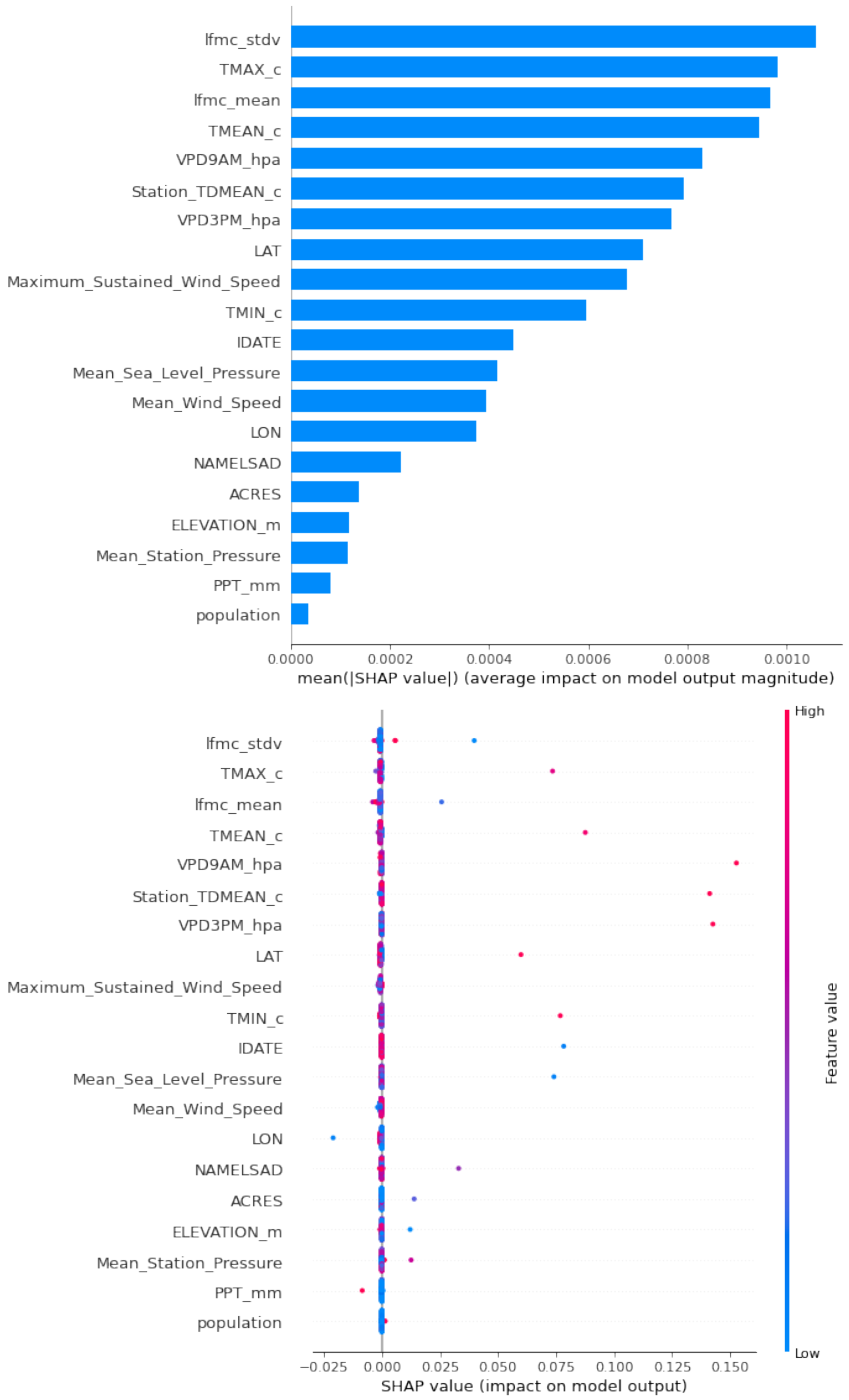
5.3. Feature Importance Derived Using Shapley Values

This section examines the results obtained by applying Shapley values, emphasizing the most crucial features and their impact on one-class ML models. These values are obtained using game theory principles and coefficients from the internal linear regression [8].

The Shapley value is a metric used to determine the average marginal contribution of each feature when considering all possible combinations (coalitions) of features [8]. For example, to calculate the Shapley value of the mean wind speed, one must evaluate all possible coalitions of features that include or exclude the mean wind speed. Each coalition’s marginal contribution of the mean wind speed to the target variable (e.g., ignition probability) is assessed. By aggregating these marginal contributions across all coalitions, the mean marginal contribution of the mean wind speed is obtained, representing its Shapley value.

Using Shapley values [8], features on the Shapley plots are arranged in descending order of importance. Hence, the feature at the top of the Shapley plot is the most important feature for predicting that activity (class). Dots on the Shapley plots correspond to an instance from the dataset. The dot’s color ranges from a low value (blue) to a high value (red). The dot’s position on the x-axis shows whether the feature for that data instance has a positive impact (to the right) or a negative impact (to the left) on the model’s prediction of a class, as measured by the Shapley value for that feature. The plot on the left in Figure 3 shows the average impact of the features on the one-class OCSVM (PyOD) ML model’s outputs for California.

Based on Figure 3, the most influential attributes include the maximum and average dew point temperatures associated with different seasons. Following this, Mean_Sea_Level_Pressure, PPT_mm, and lfmc_mean are the second set of essential features that influence wildfire prediction. For example, the temperature variables and lfmc_mean significantly impact the model output for the wildfire risk compared to the population. Also, high LFMC is more susceptible to ignition and can signal more fire spread [36]. Mean_Sea_Level_Pressure is the average level of one or more bodies of water on Earth from which elevation can be calculated. With increasing elevation, sea level pressure decreases. Wind speed and direction are both factors in the wind effect. The dry wind is one of the primary causes of wildfire spreading. The rate of wildfire spread has been estimated to be around 8% of wind speed, regardless of fuel type, especially in dry fuel moisture conditions [1].

Similar trends were found when investigating the importance of the Shapley values obtained from four of the remaining six ML models, as shown in

Table 7. Shapley value-based feature importance for the Californian dataset.

No.	Feature	One-Class SVM (scikit-learn)	One-Class SVM (PyOD)	AutoEncoder (PyOD)	Variational AutoEncoder (PyOD)	Isolation Forest (PyOD)
1	IDATE	6.36%	9.85%	1.84%	1.84%	10.26%
2	LAT	6.37%	5.90%	0.64%	0.51%	2.17%
3	LON	7.42%	3.74%	0.5%	0.59%	2.10%
4	ELEVATION_m	12.39%	0.28%	0.57%	0.41%	3.23%
5	ACRES	0.88%	4.70%	15.93%	15.94%	14.97%
6	PPT_mm	5.47%	7.13%	45.24%	45.40%	3.28%
7	TMIN_c	3.45%	7.55%	2.91%	2.99%	4.23%
8	TMEAN_c	4.45%	9.59%	4.01%	4.23%	3.21%
9	TMAX_c	6.32%	11.30%	3.64%	3.86%	10.13%
10	TDMEAN_c	5.34%	7.89%	0.84%	1.23%	2.61%
11	VPDMIN_hpa	6.77%	0.81%	2.12%	2.10%	3.86%
12	VPDMAX_hpa	6.58%	5.66%	2.94%	2.87%	7.31%
13	lfmc_mean	6.11%	6.67%	4.10%	4.05%	2.89%
14	lfmc_stdv	6.44%	4.70%	3.20%	2.69%	1.69%
15	Mean_Sea_Level_Pressure	3.62%	7.86%	1.02%	0.81%	4.91%
16	Mean_Station_Pressure	4.27%	3.32%	0.27%	0.28%	2.80%
17	Mean_Wind_Speed	2.33%	1.56%	3.00%	2.80%	3.07%
18	Maximum_Sustained_Wind_Speed	2.15%	0.91%	3.16%	3.44%	4.07%
19	NAMELSAD	1.45%	0.05%	0.29%	0.14%	1.96%
20	Population	1.86%	0.52%	3.77%	3.81%	11.26%

. The percentage value in each column of the table quantified the contribution of that feature for predicting a wildfire as measured by the Shapley value for that feature. For example, with the one-class SVM (PyOD), the contribution of TMAX_c to the prediction of a wildfire incident was 11.30% but for the same ML model Population had only a negligible contribution of 0.52%. Conversely, for the Variational AutoEncoder, the contribution of PPT_mm was 45.40%, suggesting that this feature is significant to VAE model prediction. In contrast, the Shapley value for Mean_Sea_Level_Pressure contributed only 0.28%, indicating that this feature had much lower importance for this model.

In conclusion, the results from Table 7 indicate that the features with high percentage values for each ML model should be more important in the modeling process. How exactly the features significantly influence other ML models’ outcomes should also be investigated, as demonstrated by the results of the Shapley value plot, which is presented in Figure 3.

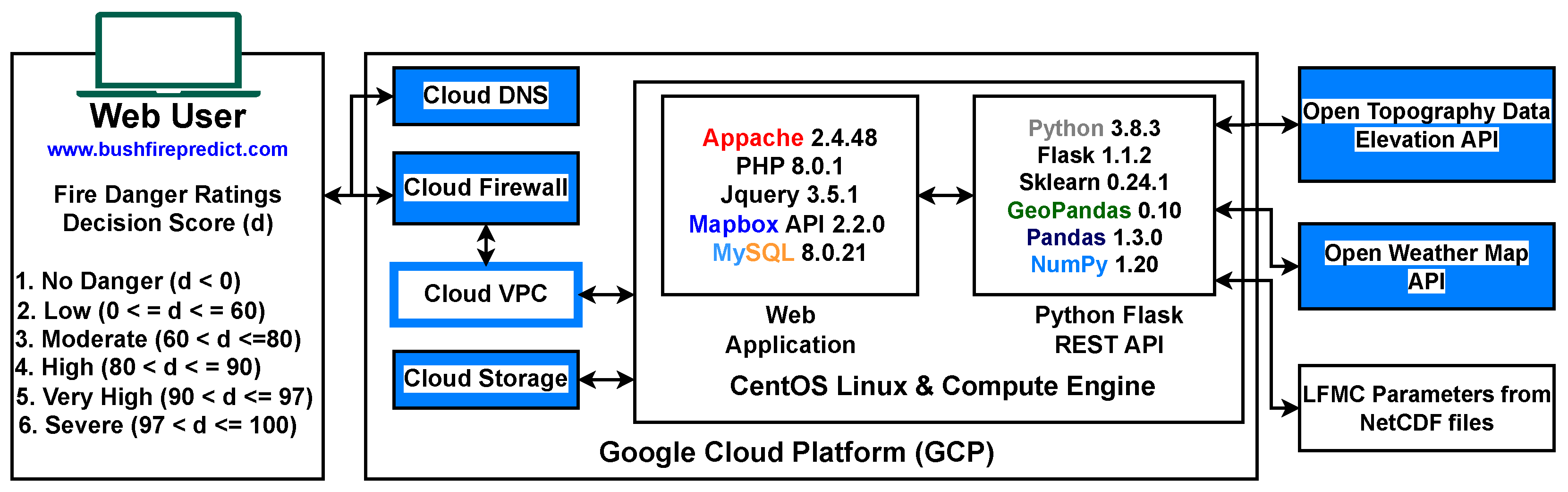
6. Deployment of Machine Learning Models

The insights gained from testing various features and models contributed to the development of a web-based application, which is described in the next section, to illustrate the effectiveness and applicability of one-class ML models. This online tool (https://www.bushfirepredict.com, accessed on 8 April 2025) serves as a novel contribution to the domain of ML-driven wildfire prediction (see Figure 4). The key objective of this research stage is to integrate the selected ML model with a REST API, which will be incorporated into the web application. This tool aims to generate long-term wildfire predictions utilizing one-class ML models, aiming to predict fire occurrences up to one week in advance for locations within California. Additionally, it offers wildfire management agencies across the globe an opportunity to evaluate wildfire prediction models in diverse regions. The tool is particularly beneficial for countries lacking dedicated wildfire forecasting systems, though it is not designed to replace existing regional wildfire prediction frameworks.

The ML model processes 20 input variables (refer to Section 4) from four key categories and six probability-based fire risk levels. These levels are defined by the decision scores (d) assigned by the one-class ML models. The six levels are as follows: No Danger (d ≤ 0), Low (0 < d ≤ 60), Moderate (60 < d ≤ 80), High (80 < d ≤ 90), Very High (90 < d ≤ 97), and Severe (97 < d ≤ 100). Each level represents a different degree of fire risk, with ‘No Danger’ indicating no immediate threat and ‘Severe’ indicating an imminent or ongoing fire. The classification of these fire risk levels aligns with the fire spread probability estimates used in the US Wildland Fire Decision Support System [51]. Historical wildfire risk assessments, as documented in [52], inform the chosen threshold values for the fire danger rating levels, which are significant as they determine the severity of the predicted fire risk. The Flask-based REST API for the web application interacts with three additional external REST APIs to facilitate wildfire prediction:

• The Open Topo Data API, a freely accessible service providing elevation data for any given latitude and longitude.
• The OpenWeather API, which offers past, present, and forecasted weather conditions globally through REST API calls.
• The USGS Earth Explorer platform, which supplies LFMC data through vegetation indices formatted for all Californian locations based on a MODIS grid.

The web-based tool is structured to provide the following core functionalities:

• The selection of historical wildfire events for model training and validate outputs. Users can also modify input parameters and analyze key contributing factors to wildfire risk as identified by the ML models.
• The ability to choose any location in California or Western Australia via an interactive map, manually input feature values, and generate wildfire risk probabilities.
• The retrieval of all predictive feature values for a seven-day period.
• The visualization of historical wildfire heatmaps based on training and testing datasets used in the ML model.

Recent technological advancements in wildfire management have been driven by the high costs and logistical challenges associated with fire suppression efforts. Among these advancements, technology-based training is pivotal in establishing standardized data-sharing frameworks and enhancing communication between fire response teams. The application of predictive modeling tools has allowed emergency responders to improve preparedness and implement preemptive measures. Equipping firefighters with the necessary training to handle wildfire emergencies remains crucial. A cost-effective and user-friendly prototype can be a valuable alternative to expensive training programs. Significant budget allocations can also be redirected toward public awareness initiatives focusing on wildfire prevention and natural fire hazards.

The Google Cloud Platform (GCP) infrastructure, which includes a virtual machine and domain hosting, is the primary cost component for maintaining the web-based tool. The required services and software are either open-source, free to use, or available under a free-tier usage policy. Deploying the tool within an on-premise local network could further reduce infrastructure expenses. The operational cost for hosting this tool is approximately NZD 42 per month, enabling wildfire forecasts up to seven days in advance (a detailed cost analysis is provided in [10] (pp. 167–168)). The system supports up to 1000 daily predictions, with each forecast extending a week ahead. The web-based tool can handle up to five prediction requests per second. Given its affordability and extensive capabilities, this deployment offers a cost-effective solution for researchers exploring wildfire prediction models. Furthermore, its adaptability allows fire management authorities to test and evaluate the system for broader public use at a minimal cost. A user-based survey was conducted to measure the tool’s effectiveness, and the corresponding findings are discussed in the next section.

7. Web-Based Prototype Evaluation

Users can access wildfire prediction capabilities through the website www.bushfire-predict.com, accessed on 8 April 2025. This online tool facilitates fire predictions in California and Western Australia for any specified location within these regions as shown in Figure 5. Users can select locations from a heatmap to forecast wildfires up to one week in advance. Furthermore, historical wildfire events can be examined using specific past incidents. ML models generate prediction results, offering both manual and automatic search options. Predictions are displayed with positive or negative labels indicating potential wildfire occurrences or the absence thereof. Additionally, potential wildfires are categorized into fire danger rating classes, ranging from No Danger to Severe levels.

The effectiveness of the web-based tool was evaluated through an 18-question survey administered to computing professionals in New Zealand. The survey covered overall design, system performance, and content clarity, among other aspects. A total of 11 participants completed the questionnaire, with an average completion time of approximately 15 min. The findings revealed that over 81% of participants primarily accessed the tool using Chrome, while some also utilized Firefox. Additionally, more than 63% of respondents expressed a high level of satisfaction, while the remaining participants rated their satisfaction as “moderate”.

When testing the mobile version across different browsers, feedback varied. While most participants found the mobile experience satisfactory, 18% were neutral, and 9% reported being highly dissatisfied. This indicates a need for the further optimization of the mobile interface. Regarding the tool’s overall design, feedback consistently rated it above average. Participants noted that data retrieval from input fields, ML-based predictions, and system response times had a high speed in terms of performance. Overall, 80% of respondents rated performance as excellent, while more than 63% provided positive feedback regarding the clarity of the input and output features and the accuracy of wildfire prediction results. These responses indicate a strong performance rating for the web-based tool (further details on the survey findings can be accessed from [10] (pp. 193–202)).

8. Threats to Validity and Limitations

We acknowledge that some uncontrolled factors might have impacted the results reported in our study. For example, the one-class ML models demonstrated high prediction accuracy for California and Western Australia instead of scaling these ML models to countrywide analyses. We underscore the crucial need for region-specific modeling due to the significant influence of varying climate and vegetation factors. This issue necessitates the frequent recalibration of the ML models to address these environmental changes. By doing this, the efficacy and reliability of these ML models in predicting wildfires would be maintained.

Next, accurate climate forecasting is critical for predicting wildfires, but climate change complicates this, limiting the ML models’ effectiveness. To mitigate this issue, we took steps to source appropriate climate data informed by relevant prior research to generate the datasets. However, we are optimistic about the potential of data produced by more recent climate forecasting models to mitigate this problem in the future.

Furthermore, location-specific granular data were interpolated from station-based weather data. However, including more specific location-based data acquired from hand-held sensors or wireless sensor networks might improve model accuracy. It is important to note that adopting higher-resolution satellite or drone-based images could also enhance LFMC values, but this enhancement comes with a higher financial cost that needs to be considered.

Another potential threat to the accuracy of our ML models was over-fitting. Over-fitting occurs when a model learns the training data too well, to the point that it negatively impacts its ability to predict new, unseen data. To mitigate this risk, our methodology included a five-fold CV when establishing the best hyper-parameters for a specific one-class ML model type. This approach allowed us to thoroughly assess the best one-class ML model performance using 20 times five-fold CV, thereby reducing the risk of over-fitting and increasing the model’s ability to generalize to unseen data. It is crucial to remember that the predictive models in question use a consistent algorithmic approach and methodological framework to guarantee consistency in their predictive processes. The fact that different geographic regions have varying feature sets presents a problem too, because some features are not always included in both models. This discrepancy can affect how broadly applicable the forecasts are, necessitating more refinement and adjustment. Additionally, implementing advanced deep learning models requires a significant amount of computing power and data availability, which may have practical restrictions. Additional experimental evaluations are required to increase the robustness and generalizability of these models’ effectiveness.

Finally, the one-class and two-class ML models were built using currently available Python libraries, implementing existing one-class and two-class learning algorithms. While these libraries limited the scope of applying other appropriate ML algorithms for wildfire prediction, they also did not consider non-ML-based approaches. Wildfire prediction using physical models [53] or statistical models [54] might yield slightly different results with the same dataset, pointing to a limitation in using ML for wildfire prediction. However, these non-ML-based approaches have their own strengths and could be valuable in certain contexts. Despite these considerations, our methodology was consistently applied across different geographic locations, supporting model re-usability. The future testing of our methodology in diverse environmental and geographical contexts can further validate our research approach.

9. Conclusions and Future Work

In conclusion, historical wildfire occurrences in California and Western Australia were represented using 20 distinct features. Seven one-class ML algorithms were utilized to train multiple models, and hyper-parameter tuning was performed to optimize their performance. Model validation was conducted using 20 × five-fold cross-validation (CV), a rigorous process that involves dividing the data into 20 sets, training the model on 19 sets, and testing it on the remaining set, repeated 20 times. The test Accuracy values ranged between 0.90 and 1.00, indicating the robustness of the models. These results indicate that the ML models achieved consistently high predictive performance across both datasets. Precision, Recall, and F1-Score metrics were used to assess their effectiveness.

Our study not only delves into the development of ML-based wildfire prediction models but also uncovers the key predictive features that fuel wildfire ignition. These findings, in line with previous research, shed light on the intricate relationship between these features and wildfire risk, sparking further interest in this field.

Moreover, we have introduced a web-based prototype that harnesses the power of the best-performing ML models to simplify wildfire occurrence mapping. This innovative tool, designed for both the general public and wildfire management authorities, holds promise for the future of wildfire management.

The enhanced OCSVM model, seamlessly integrated into the system via a Flask API, has been deployed on a web server at minimal cost, with the potential for future scalability. This reassures the audience about the long-term viability of the system. However, the methodology employed in this research may differ from other domains with unique characteristics and ML techniques, which will be explored in future work to address these variations. Additionally, the usability of the web-based tool was evaluated to assess its practical effectiveness.

Since this study was limited to two datasets, future research will focus on expanding wildfire datasets from other countries, incorporating potentially different features. The top-ranked features derived from these ML models using Shapley values may be compared with our existing findings to determine how feature contributions to wildfire risk vary by location. Similarly, investigating which hyper-parameters play a critical role in producing high-performing ML models is an avenue for further research, especially given recent advancements proposed by [55] for more computationally efficient hyper-parameter optimization.

For future directions, we plan to enhance the web-based prototype by integrating additional methodologies, such as Large Language Models (LLMs), to model wildfire event sequences and improve wildfire occurrence mapping. The intended audience for this tool remains both the general public and wildfire response agencies. Such a system has the potential to contribute to existing wildfire early detection strategies, aiding efforts to mitigate this global issue.

References

1. Jain, P.; Coogan, S.C.; Subramanian, S.G.; Crowley, M.; Taylor, S.; Flannigan, M.D. A review of machine learning applications in wildfire science and management. Environ. Rev. 2020, 28, 478–505. [Google Scholar] [CrossRef]
2. European Centre for Medium-Range Weather Forecasts. 2024 Was the Warmest Year on Record, Copernicus Data Show. Available online: https://www.ecmwf.int/en/about/media-centre/news/2025/2024-was-warmest-year-record-copernicus-data-show (accessed on 20 January 2025).
3. Miller, C.; Hilton, J.; Sullivan, A.; Prakash, M. SPARK—A Bushfire Spread Prediction Tool. In Environmental Software Systems. Infrastructures, Services and Applications; Denzer, R., Argent, R.M., Schimak, G., Hřebíček, J., Eds.; Springer International Publishing: Cham, Switzerland, 2015; pp. 262–271. [Google Scholar] [CrossRef]
4. Bowman, D.M.J.S.; Williamson, G.J.; Price, O.F.; Ndalila, M.N.; Bradstock, R.A. Australian forests, megafires and the risk of dwindling carbon stocks. Plant Cell Environ. 2021, 44, 347–355. [Google Scholar] [CrossRef]
5. Chandola, V.; Banerjee, A.; Kumar, V. Anomaly detection: A survey. ACM Comput. Surv. 2009, 41, 1–58. [Google Scholar] [CrossRef]
6. Khan, S.S.; Madden, M.G. One-Class Classification: Taxonomy of Study and Review of Techniques. Knowl. Eng. Rev. 2014, 29, 345–374. [Google Scholar] [CrossRef]
7. Nguyen, P.T.; Nguyen, T.T.; Nguyen, N.C.; Le, T.T. Multiclass breast cancer classification using convolutional neural network. In Proceedings of the 2019 International Symposium on Electrical and Electronics Engineering (ISEE), Ho Chi Minh City, Vietnam, 10–12 October 2019; IEEE: Piscataway, NJ, USA, 2019; pp. 130–134. [Google Scholar]
8. Lundberg, S.M.; Lee, S.I. A unified approach to interpreting model predictions. In Proceedings of the 31st International Conference on Neural Information Processing Systems, Red Hook, NY, USA, 4–9 December 2017; pp. 4768–4777. [Google Scholar]
9. Tyukavina, A.; Potapov, P.; Hansen, M.C.; Pickens, A.H.; Stehman, S.V.; Turubanova, S.; Parker, D.; Zalles, V.; Lima, A.; Kommareddy, I.; et al. Global Trends of Forest Loss Due to Fire from 2001 to 2019. Front. Remote Sens. 2022, 3, 825190. [Google Scholar] [CrossRef]
10. Ismail, F.N. Novel Machine Learning Approaches for Wildfire Prediction to Overcome the Drawbacks of Equation-Based Forecasting. Ph.D. Thesis, University of Otago, Dunedin, New Zealand, 2022. [Google Scholar]
11. Ismail, F.N.; Sengupta, A.; Woodford, B.J.; Licorish, S.A. A Comparison of One-Class Versus Two-Class Machine Learning Models for Wildfire Prediction in California. In Proceedings of the Australasian Conference on Data Science and Machine Learning—AusDM 2023, Auckland, New Zealand, 11–13 December 2023; pp. 239–253. [Google Scholar]
12. Ismail, F.N.; Woodford, B.J.; Licorish, S.A.; Miller, A.D. An assessment of existing wildfire danger indices in comparison to one-class machine learning models. Nat. Hazards 2024, 120, 14837–14868. [Google Scholar] [CrossRef]
13. Ismail, F.N.; Amarasoma, S. One-class Classification-Based Machine Learning Model for Estimating the Probability of Wildfire Risk. Procedia Comput. Sci. 2023, 222, 341–352. [Google Scholar] [CrossRef]
14. Cortes, C.; Vapnik, V. Support-Vector Networks. Mach. Learn. 1995, 20, 273–297. [Google Scholar] [CrossRef]
15. Tax, D.M.; Duin, R.P. Support vector domain description. Pattern Recognit. Lett. 1999, 20, 1191–1199. [Google Scholar] [CrossRef]
16. Liu, F.T.; Ting, K.M.; Zhou, Z. Isolation Forest. In Proceedings of the 2008 Eighth IEEE International Conference on Data Mining, Piscataway, NJ, USA, 15–19 December 2008; pp. 413–422. [Google Scholar] [CrossRef]
17. Alkhatib, R.; Sahwan, W.; Alkhatieb, A.; Schütt, B. A Brief Review of Machine Learning Algorithms in Forest Fires Science. Appl. Sci. 2023, 13, 8275. [Google Scholar] [CrossRef]
18. Ntinopoulos, N.; Sakellariou, S.; Christopoulou, O.; Sfougaris, A. Fusion of Remotely-Sensed Fire-Related Indices for Wildfire Prediction through the Contribution of Artificial Intelligence. Sustainability 2023, 15, 11527. [Google Scholar] [CrossRef]
19. Patterson, J.; Gibson, A. Deep Learning: A Practitioner’s Approach; O’Reilly Media, Inc.: Sebastopol, CA, USA, 2017. [Google Scholar]
20. Ruff, L.; Vandermeulen, R.; Goernitz, N.; Deecke, L.; Siddiqui, S.A.; Binder, A.; Müller, E.; Kloft, M. Deep One-Class Classification. In Proceedings of the 35th International Conference on Machine Learning, Stockholm, Sweden, 10–15 July 2018; pp. 4393–4402. [Google Scholar]
21. Kim, S.; Choi, Y.; Lee, M. Deep learning with support vector data description. Neurocomputing 2015, 165, 111–117. [Google Scholar] [CrossRef]
22. Zenati, H.; Romain, M.; Foo, C.S.; Lecouat, B.; Chandrasekhar, V. Adversarially learned anomaly detection. In Proceedings of the 2018 IEEE International Conference on Data Mining (ICDM), Singapore, 17–20 November 2018; IEEE Press: Piscataway, NJ, USA, 2018; pp. 727–736. [Google Scholar] [CrossRef]
23. Pedregosa, F.; Varoquaux, G.; Gramfort, A.; Michel, V.; Thirion, B.; Grisel, O.; Blondel, M.; Prettenhofer, P.; Weiss, R.; Dubourg, V.; et al. Scikit-learn: Machine Learning in Python. J. Mach. Learn. Res. 2011, 12, 2825–2830. [Google Scholar]
24. Zhao, Y.; Nasrullah, Z.; Li, Z. PyOD: A Python Toolbox for Scalable Outlier Detection. J. Mach. Learn. Res. 2019, 20, 1–7. [Google Scholar]
25. Seliya, N.; Zadeh, A.A.; Khoshgoftaar, T.M. A literature review on one-class classification and its potential applications in big data. J. Big Data 2021, 8, 1–31. [Google Scholar] [CrossRef]
26. Schölkopf, B.; Platt, J.C.; Shawe-Taylor, J.; Smola, A.J.; Williamson, R.C. Estimating the support of a high-dimensional distribution. Neural Comput. 2001, 13, 1443–1471. [Google Scholar] [CrossRef]
27. Bishop, C. Neural Networks for Pattern Recognition; Oxford University Press: Cary, NC, USA, 1995. [Google Scholar]
28. Jiang, M.F.; Tseng, S.; Su, C. Two-phase clustering process for outliers detection. Pattern Recognit. Lett. 2001, 22, 691–700. [Google Scholar] [CrossRef]
29. Salekshahrezaee, Z.; Leevy, J.L.; Khoshgoftaar, T.M. A reconstruction error-based framework for label noise detection. J. Big Data 2021, 8, 1–16. [Google Scholar] [CrossRef]
30. Japkowicz, N.; Myers, C.; Gluck, M. A novelty detection approach to classification. In IJCAI; Citeseer: Princeton, NJ, USA, 1995; Volume 1, pp. 518–523. [Google Scholar]
31. Désir, C.; Bernard, S.; Petitjean, C.; Heutte, L. One class random forests. Pattern Recognit. 2013, 46, 3490–3506. [Google Scholar] [CrossRef]
32. Krawczyk, B.; Wozniak, M.; Cyganek, B. Clustering-based ensembles for one-class classification. Inf. Sci. 2013, 264, 182–195. [Google Scholar] [CrossRef]
33. Bergstra, J.; Yamins, D.; Cox, D.D. Making a Science of Model Search: Hyperparameter Optimization in Hundreds of Dimensions for Vision Architectures. In Proceedings of the 30th International Conference on International Conference on Machine Learning, Atlanta, GA, USA, 16–21 June 2013; Volume 28, pp. I-115–I-123. [Google Scholar]
34. Abdollahi, A.; Pradhan, B. Explainable artificial intelligence (XAI) for interpreting the contributing factors feed into the wildfire susceptibility prediction model. Sci. Total Environ. 2023, 879, 163004. [Google Scholar] [CrossRef]
35. Tonini, M.; D’Andrea, M.; Biondi, G.; Degli Esposti, S.; Trucchia, A.; Fiorucci, P. A Machine Learning-Based Approach for Wildfire Susceptibility Mapping. The Case Study of the Liguria Region in Italy. Geosciences 2020, 10, 105. [Google Scholar] [CrossRef]
36. Jaafari, A.; Pourghasemi, H.R. 28—Factors Influencing Regional-Scale Wildfire Probability in Iran: An Application of Random Forest and Support Vector Machine. In Spatial Modeling in GIS and R for Earth and Environmental Sciences; Pourghasemi, H.R., Gokceoglu, C., Eds.; Elsevier: Amsterdam, The Netherlands, 2019; pp. 607–619. [Google Scholar] [CrossRef]
37. Donovan, G.H.; Prestemon, J.P.; Gebert, K. The Effect of Newspaper Coverage and Political Pressure on Wildfire Suppression Costs. Soc. Nat. Resour. 2011, 24, 785–798. [Google Scholar] [CrossRef]
38. Jiménez-Ruano, A.; Mimbrero, M.R.; de la Riva Fernández, J. Understanding wildfires in mainland Spain. A comprehensive analysis of fire regime features in a climate-human context. Appl. Geogr. 2017, 89, 100–111. [Google Scholar] [CrossRef]
39. Papadopoulos, A.; Paschalidou, A.; Kassomenos, P.; McGregor, G. On the association between synoptic circulation and wildfires in the Eastern Mediterranean. Theor. Appl. Climatol. 2014, 115, 483–501. [Google Scholar] [CrossRef]
40. Nunes, A.; Lourenço, L.; Meira Castro, A.C. Exploring spatial patterns and drivers of forest fires in Portugal (1980–2014). Sci. Total Environ. 2016, 573, 1190–1202. [Google Scholar] [CrossRef]
41. Stein, M.L. Interpolation of Spatial Data: Some Theory for Kriging; Springer Series in Statistics; Springer: New York, NY, USA, 1999. [Google Scholar] [CrossRef]
42. Tadić, J.M.; Ilić, V.; Biraud, S. Examination of geostatistical and machine-learning techniques as interpolators in anisotropic atmospheric environments. Atmos. Environ. 2015, 111, 28–38. [Google Scholar] [CrossRef]
43. Tien Bui, D.; Bui, Q.T.; Nguyen, Q.P.; Pradhan, B.; Nampak, H.; Trinh, P.T. A hybrid artificial intelligence approach using GIS-based neural-fuzzy inference system and particle swarm optimization for forest fire susceptibility modeling at a tropical area. Agric. For. Meteorol. 2017, 233, 32–44. [Google Scholar] [CrossRef]
44. Sayad, Y.O.; Mousannif, H.; Al Moatassime, H. Predictive modeling of wildfires: A new dataset and machine learning approach. Fire Saf. J. 2019, 104, 130–146. [Google Scholar] [CrossRef]
45. Nhu, V.H.; Shirzadi, A.; Shahabi, H.; Singh, S.K.; Al-Ansari, N.; Clague, J.J.; Jaafari, A.; Chen, W.; Miraki, S.; Dou, J.; et al. Shallow Landslide Susceptibility Mapping: A Comparison between Logistic Model Tree, Logistic Regression, Naïve Bayes Tree, Artificial Neural Network, and Support Vector Machine Algorithms. Int. J. Environ. Res. Public Health 2020, 17, 2749. [Google Scholar] [CrossRef]
46. Ghorbanzadeh, O.; Valizadeh Kamran, K.; Blaschke, T.; Aryal, J.; Naboureh, A.; Einali, J.; Bian, J. Spatial Prediction of Wildfire Susceptibility Using Field Survey GPS Data and Machine Learning Approaches. Fire 2019, 2, 43. [Google Scholar] [CrossRef]
47. Michael, Y.; Helman, D.; Glickman, O.; Gabay, D.; Brenner, S.; Lensky, I.M. Forecasting fire risk with machine learning and dynamic information derived from satellite vegetation index time-series. Sci. Total Environ. 2021, 764, 142844. [Google Scholar] [CrossRef] [PubMed]
48. Goldarag, Y.; Mohammadzadeh, A.; Ardakani, A. Fire Risk Assessment Using Neural Network and Logistic Regression. J. Indian Soc. Remote Sens. 2016, 44, 1–10. [Google Scholar] [CrossRef]
49. de Bem, P.; de Carvalho Júnior, O.; Matricardi, E.; Guimarães, R.; Gomes, R. Predicting wildfire vulnerability using logistic regression and artificial neural networks: A case study in Brazil. Int. J. Wildland Fire 2018, 28, 35–45. [Google Scholar] [CrossRef]
50. Ma, J.; Cheng, J.; Jiang, F.; Gan, V.; Wang, M.; Zhai, C. Real-time detection of wildfire risk caused by powerline vegetation faults using advanced machine learning techniques. Adv. Eng. Inform. 2020, 44, 101070. [Google Scholar] [CrossRef]
51. Jolly, W.M.; Freeborn, P.H.; Page, W.G.; Butler, B.W. Severe Fire Danger Index: A Forecastable Metric to Inform Firefighter and Community Wildfire Risk Management. Fire 2019, 2, 47. [Google Scholar] [CrossRef]
52. National Interagency Fire Center; National Wildfire Coordinating Group (NWCG). Interagency Standards for Fire and Fire Aviation Operations; Createspace Independent Publishing Platform, Great Basin Cache Supply Office: Boise, ID, USA, 2019.
53. Sullivan, A.L. Physical Modelling of Wildland Fires. In Encyclopedia of Wildfires and Wildland-Urban Interface (WUI) Fires; Springer International Publishing: Cham, Switzerlands, 2019; pp. 1–8. ISBN 978-3-319-51727-8. [Google Scholar] [CrossRef]
54. Taylor, S.W.; Woolford, D.G.; Dean, C.B.; Martell, D.L. Wildfire Prediction to Inform Fire Management: Statistical Science Challenges. Stat. Sci. 2013, 28, 586–615. [Google Scholar] [CrossRef]
55. Watanabe, S.; Bansal, A.; Hutter, F. PED-ANOVA: Efficiently Quantifying Hyperparameter Importance in Arbitrary Subspaces. In Proceedings of the Thirty-Second International Joint Conference on Artificial Intelligence, IJCAI-23, Macao, China, 19–25 August 2023; pp. 4389–4396. [Google Scholar] [CrossRef]
Figure 1. Comparison between one-class classification (a) and two-class classification (b). Unlike one-class classification models, two-class classification models incorporate both inlier (positive) and outlier labels, explicitly distinguishing between the two classes.
Atmosphere 16 00441 g001
Figure 2. The process of building a wildfire prediction model involves various steps from data preparation, data pre-processing, model generation using one-class ML, model validation, and deploying ML models through a web-based tool.
Atmosphere 16 00441 g002
Figure 3. Feature importance ranked by mean absolute SHAP values generated from the OCSVM PyOD model (top) and corresponding SHAP summary plot illustrating individual data points with respective feature values ranging from low to high (bottom).
Atmosphere 16 00441 g003
Figure 4. The architecture of the deployed ML model, generating wildfire risk predictions across six fire danger categories.
Atmosphere 16 00441 g004
Figure 5. Inyo 30 June 2012 fire event with main input features.
Atmosphere 16 00441 g005