Abstract
Efficiently mapping hourly air quality at a fine scale (25 m) remains a computational challenge. This difficulty is heightened when aiming to accurately capture industrial plumes and time-varying traffic emissions. This paper presents a method for generating hourly pollutant concentration maps across an entire region for operational applications. Our approach assumes that concentration maps can be decomposed into three components: traffic concentrations, industrial concentrations and a residual “background” concentrations component. The background concentration is estimated using established fine-scale mapping methods involving ADMS-Urban dispersion simulations. Meanwhile, the traffic and industrial layers are derived using a KNN-based approach applied to a sample of hourly ADMS-Urban simulations. This method enhances the representation of industrial plumes and the temporal variability in traffic emissions while maintaining computational efficiency, making it suitable for the operational production of hourly air quality maps in the Hauts-de-France region (France).
1. Introduction
The global strategy for air quality monitoring relies on monitoring stations to collect data in real time and implement policies to protect both human health and the environment. To ensure citizens are informed about the air quality they breathe, especially in areas outside traditional monitoring networks, air quality modeling techniques have been developed over the past decade. These spatial and temporal models offer valuable insights into the progression of air quality, enabling stakeholders to make informed decisions and encouraging individuals to modify their behaviors accordingly. This is why the revised Ambient Air Quality Directive [1] highlights the critical role of both monitoring and modeling in ensuring adherence to stricter air quality standards. By reinforcing requirements for air quality monitoring and modeling, the directive enhances the ability to evaluate compliance with the new standards and supports more effective actions to address violations. These strengthened regulations aim to provide a clearer understanding of air quality, guiding authorities in their efforts to meet the 2030 air quality targets. With these tools in hand, authorities can better assess pollution levels, respond promptly and work towards the EU’s goal of zero pollution by 2050.
Air quality models employ mathematical and numerical methods to simulate the physical and chemical processes that influence the behavior of air pollutants in the atmosphere. These models rely on meteorological data and other sources of information, such as emission rates and stack heights, to predict how pollutants disperse and interact with each other in the environment. Thus, air pollution modeling depends on understanding the interactions between emissions, meteorology and atmospheric concentrations to predict pollutant dispersion and assess their effects on the population’s health and the environment. Various models are used, such as Gaussian models for the dispersion of emissions [2], Lagrangian models with particles’ trajectories tracking [3], Eulerian models to analyze pollution on fixed numerical grids [4] and chemical transport models (CTMs) that combine transport mechanisms with atmospheric chemistry [5]. In their study, Jacquinot et al. [6] introduce a method for efficiently generating fine-scale daily mappings of pollutant concentrations. This method has shown promise in providing detailed information on air quality variations at a local level. However, upon closer examination, we observe that the approach encounters difficulties in accurately representing certain key sources of pollution in the Hauts-de-France region, specifically industrial plumes and the temporal fluctuations associated with traffic emissions. This may be explained by the low number of traffic stations in our region and the significant presence of potential industrial sources, which are more strongly influenced by prevailing weather conditions compared to the South of France. By more effectively accounting for local industrial, agricultural and climatic factors, this model could provide policymakers with data that are more representative and globally applicable. This kind of approach would better address the complex spatial and temporal patterns of these sources, which often pose challenges to traditional modeling techniques [7]. Industrial plumes, for example, often involve concentrated emissions that can vary in intensity and direction depending on weather conditions, while traffic emissions display marked daily and weekly cycles, linked to rush hours and commuting patterns. It was already noted that the traditional models often struggle with complex terrains and may not accurately capture the nonlinear relationships between pollutant concentrations and their sources. Some recent studies have shown that, even when highly precise data, such as satellite observations, are integrated, it remains difficult to accurately reproduce the diffusion of pollutants due to biases related to wind speed and direction [8]. Modeling at a fine spatial and temporal resolution often requires larger volumes of data to process and consequently also significantly higher computational resources. The complexity of atmospheric processes, including turbulence, chemical reactions and interactions with topography, further amplifies the computational burden. As a result, achieving high precision while maintaining reasonable simulation times remains a major challenge. To address this gap, we propose an alternative approach that combines statistical and machine learning methods with the existing fine-scale mapping framework. Recent studies suggest that machine learning tools can significantly improve the accuracy of predictions [9,10]. Our proposed statistical technique is designed to enhance the representation of both industrial emissions and traffic-related pollution. By integrating data on industrial activity and traffic patterns, along with statistical corrections for known emission profiles, our method can more effectively capture the variations in pollutant concentrations caused by these specific sources. This approach not only improves the precision of concentration mappings, but also provides a more nuanced understanding of air quality dynamics at the local scale, particularly in areas where industrial or traffic emissions are significant contributors. The core of the method is based on the k-nearest neighbor algorithm (KNN), which was already successfully applied for the predictions of air quality [11,12]. To the best of our knowledge, the method we propose is the first to introduce a metamodel based on the ADMS-Urban model, focusing on the two most variable proximity sectors, namely traffic and industry. This approach allows for the efficient use of computational resources to generate high-resolution maps.
2. Materials and Methods
2.1. Site Description
The study area is located in northern France, covering an area of around 31,800 km² in the Hauts-de-France (HDF) region (Figure 1). The area is populated with nearly 6 million people. The largest cities include Lille (over 230,000 inhabitants), Amiens (around 135,000 inhabitants) and Dunkirk (approximately 86,000 inhabitants). The northern part of the study area borders the North Sea, characterized by a maritime climate and strong industrial activity, particularly around Dunkirk’s and Calais port area. In contrast, the southern part consists of agricultural plains and rolling landscapes, with lower population density and less industrial influence. Nevertheless, this part may be affected by pollution coming from the Paris region. Urban and industrial zones within the study area often face poor air quality, mostly due to elevated concentrations of , , and .
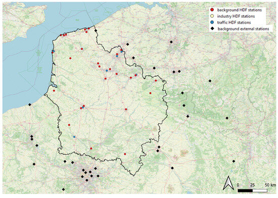
Figure 1.
Regional monitoring stations used to collect background, traffic and industrial concentration data for and in the Hauts-de-France (HDF) region. These stations might have different implantations, namely urban, suburban and rural.
2.2. Air Quality Monitoring in the Hauts-De-France Region
In the Hauts-de-France region, air quality is originally monitored using an ensemble of 45 monitoring stations distributed across the five departments Nord, Pas-de-Calais, Somme, Aisne and Oise, that collect concentration data for several air pollutants among which Ozone (), nitrogen dioxide () and particulate matter ( and ). These pollutants are used to calculate the hourly air quality index (ICAIRh), a simplified indicator of global air quality [13]. This index provides continuous air quality estimations throughout the day, allowing citizens to better anticipate changes in air quality, adjust their outdoor activities and outings and limit their exposure to pollution to protect their health.
Each monitoring station is assigned a specific site category, which refers to the environment of the station (rural, suburban or urban) based on the surrounding population and building density. Additionally, the corresponding measurements are categorized by their "influence" (background, industrial or traffic), depending on the likelihood of being affected by industrial or traffic emissions. These criteria are based on those introduced by the European Environment Agency in their classification and criteria for the inclusion of air quality monitoring stations in their assessment products (https://www.eea.europa.eu/en/topics/in-depth/air-pollution/monitoring-station-classifications-and-criteria, (accessed on 25 March 2025)).
In the present paper, we present the method for constructing hourly fine-scale concentration maps using concentration data measured at background monitoring stations, and for the sake of clarity we focus on two pollutants to illustrate the procedure, namely and . Figure 1 shows the geographical distribution of the regional monitoring stations where concentration measurements for and are collected.
2.3. Fine-Scale Regional Concentration Maps Construction
The different steps in the following subsections outline the methodology used to develop fine-scale pollution mapping. The method can be summarized in the following steps: first, the ADMS-Urban model is used to construct annual maps with separate outputs for traffic and industrial sectors’ contributions (Section 2.3.2). Then, hourly maps are constructed using, on one hand, the AZUR method [6] for the background concentration (Section 2.3.3), and on the other hand, a k-nearest-neighbor (KNN) statistical approach to add traffic and industrial contributions (Section 2.3.4). Last, the resulting maps are evaluated in the next section by comparing predictions with measures at the stations (Section 3.4).
2.3.1. Additivity Hypothesis and Methodology
The strategy we adopt is based on the following key additivity hypothesis: we assume that the pollutant concentration at a given location in space and a given time t, denoted and expressed in μg/, can be decomposed as
where we identify the following:
- The concentration linked to a contribution of road traffic emissions, denoted ;
- The concentration linked to a contribution of industrial emissions, denoted ;
- A part , which corresponds to the residual concentration that does not come from traffic or industrial sectors.
We assume that these three parts can be added with each other to account for the total observed concentration. Note that many sources of emissions other than traffic or industrial—such as emissions from heating, the agricultural sector, as well as natural emissions associated to dust or forest fires—are included in the background layer.
The above decomposition translates into a methodology divided into the following two main steps. For each hour of the day, we perform the following:
- 1.
- The construction of a background concentration map , resulting from a spatialization of the background concentrations measured at the monitoring stations depicted on Figure 1 (Section 2.3.2 and Section 2.3.3);
- 2.
- The estimation of the traffic and industrial layers and , using a KNN statistical approach applied to the outputs of numerical simulations of regional dispersion with the software ADMS-Urban (Section 2.3.4).
2.3.2. Annual Concentration Maps with ADMS-Urban
ADMS-Urban (https://www.cerc.co.uk/environmental-software/ADMS-Urban-model.html, (accessed on 15 January 2025)) is a numerical model originally developed in the UK by the Cambridge Environmental Research Consultants (CERCs) and is dedicated to the simulation of pollutant dispersion at the urban scale [14,15]. It belongs to the family of so-called Gaussian models, which are based on a statistical representation of scalar plumes and dispersion processes [16] and may efficiently provide estimates of pollution impacts in emergency situations. Among its many features, ADMS-Urban deals with hourly sequential or statistical meteorological data, allows for the representation of point-wise, linear and volumetric emissions sources, incorporates many physical features such as the advanced representation of canyon dynamics, photochemistry, a vertical representation of the atmospheric boundary layer, and accounts for the influence of three-dimensional buildings on the dispersion of industrial plumes.
Yearly dispersion simulations on a 25 m resolution grid are performed with ADMS-Urban (version 5.0) on the Hauts-de-France region (France) using annual emissions inventories (made by Atmo Hauts-de-France) along with meteorological data gathered from the monitoring stations of Meteo-France and completed with data from meteorological models AROME (https://www.umr-cnrm.fr/spip.php?article120&lang=en, (accessed on 15 January 2025)) and WRF (https://www.mmm.ucar.edu/models/wrf, (accessed on 15 January 2025)). Two adjustment steps are conducted on the yearly averaged maps obtained with ADMS-Urban: first, a linear bias correction informed by the concentration measures at background stations along with other geographical variables is applied, and second, yearly averaged concentration measured values are enforced at the stations using either kriging with external drift [17] or inverse distance interpolation [18].
The KNN strategy mentioned at the beginning of the section relies on a collection of data to predict hourly traffic and industrial contributions (see the dedicated Section 2.3.4). These data consist in a sample of historical data for the traffic and industrial layers and are constructed using an additional ADMS-Urban run covering the year 2022. To save some computational time, only 6 months of the year 2022 are simulated (with regular date spacing over the year), while capturing various and most representative meteorological conditions. Briefly, the most representative periods were selected using an analysis conducted on a weekly basis, identifying the most representative weeks for each season. Representativeness was quantified by comparing the hourly value distributions of wind speed, wind direction, relative humidity, precipitation and temperature. Two representativeness criteria were compared: the Kolmogorov–Smirnov test statistic and the Anderson–Darling test statistic. An example of such traffic and industrial layers is show in Figure 2 to evidence the contribution of each sector to the background concentration map constructed with the AZUR framework.
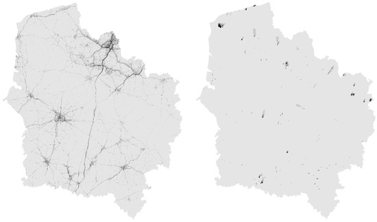
Figure 2.
Examples of traffic (left) and industrial (right) layers extracted from the sample of historical data for the prevision of the hourly concentration over the Hauts-de-France region for the targeted date of 4 February 2025 at 11:00 a.m. This figure is not meant to provide quantitative information about the concentrations but only qualitative information about the geographical distribution of traffic and industrial contributions.
2.3.3. Hourly Background Concentration Maps with AZUR
For a given hour of the day, a fine-scale map is constructed for the hourly average background concentration , using the annual map (cf. Section 2.3.2) along with the method proposed by Jacquinot et al. [6]. This method was designed to facilitate the estimation of fine-scale daily concentration map, and only requires an annual average map at the targeted spatial resolution, as well as yearly measurement data at the stations.
To understand the essence of the approach, first note that daily concentration values—defined as daily maximum or daily averaged depending on the considered pollutant—follow a statistical distribution and each daily value available in measured datasets can be seen as a decile of the underlying distribution. Denote such a decile, where p is its rank, defined as the proportion of daily values below . Jacquinot et al. [6] compared the ratios of yearly averages —where is the yearly average of the concentration values at the station s—with those of daily values for every pair of stations . They observed that the daily ratios are a function of the yearly ratio and the rank p, which is estimated using a polynomial model:
where N is the degree of the polynomial and the ’s are coefficients to be fitted using historical measurement data. Equation (2) can be used to estimate the value of a decile at an arbitrary location from the value at a neighboring station s, denoted , as follows:
where the rank p should be estimated using data at the station s, and and are obtained from the annual average map mentioned above and from the measurements, respectively. Note that, for this formula to work, the estimated concentration and the reference measure— and , respectively—should have the same rank p in the distribution of daily values. The AZUR method assumes that this is true close to the stations, and proposes the following global estimate for the daily concentration values:
with i ranging over the available measuring stations, and the weights ’s calculated as the inverse distance of s to each .
Further details can be found in the article by Jacquinot et al. [6], where the authors demonstrate that their interpolation method performs as well as kriging for the prediction of daily maxima on Provence-Alpes-Côte d’Azur region, France.
We use the AZUR method in our study to compute hourly concentration values instead of daily values, and in order to prevent possible issues associated to missing data among regional monitoring stations, we use external background measures from neighboring regions (Ile-de-France, Grand Est, Normandy as well as Belgium, see black dots on Figure 1).
2.3.4. Hourly Traffic and Industrial Contributions with KNN
Prediction from a Sample of Historical Data
After the calculation of the background component of the hourly pollutant concentration map, appropriate industrial and traffic layers defined in Equation (1) should be estimated. The idea of our approach is to exploit an additional run of ADMS-Urban to compute concentration maps with a time step of one hour over the year with a sectorial decomposition of the outputs. This yields a sample of hourly averaged maps of and and is referred to as “historical data” in the following. We denote the number of observed couples , and the set of observation dates.
Pollution resulting from road traffic at a given time in the year is highly dependent on the meteorological conditions—the amount of wind and rain for instance—and on the flow of vehicles, which depends on calendar parameters—hour, day, month, etc. Industrial emissions also driven by calendar and meteorological parameters, in particular the atmospheric stability, significantly impacts scalar plume dynamics. Consequently, calendar parameters and physical quantities associated to the meteorological conditions are the main factors that are assumed to determine traffic and industrial concentration layers.
From the above considerations, we assume that each element of the sample of historical data can be associated to a set of coordinates in the space of calendar and meteorological parameters. Denoting q the number of these parameters, each observation of the sample of historical data corresponds to a point where each is a calendar or meteorological parameter, that depends on the date of the observation t.
To compute a fine-scale concentration map for a given hour of the year, knowing the meteorological conditions, we do not need to run an additional ADMS-Urban simulation, which is time-consuming. Instead, we can select layers from historical data where the calendar and meteorological parameters are the most similar to those of the target date. To do so, we compare the meteorological forecasts of the target prediction date (derived from WRF data) and the meteorological conditions of the historical data (meteorological data registered by ADMS-Urban additional run) and measure the similarity between these two data sources.
This approach corresponds to a k-nearest neighbors (KNN [19]) regression strategy with , and provides an estimate of the and layers for a target date from the meteorological and calendar variables. Denoting the targeted date at which we want to compute and , the KNN provides the following predictor of the traffic and industrial layers:
where is chosen so as to minimize the distance between the set and the targeted coordinates :
where denotes the Euclidean distance in :
Dealing with the Spatial Variability of the Regional Weather
The meteorological conditions significantly vary across the region during the year, which makes it debatable to select historical layers from a single date . Indeed, it is unlikely that the meteorological conditions observed at the targeted date across the whole region will be comparable to those observed at some past date everywhere. Even though the distance might be minimized, in the absolute the meteorological conditions might still be very different locally.
To minimize potential discrepancies, we divided the Hauts-de-France region into 10 geographical areas. These areas were defined to capture the regional variability of weather events through clustering and rationalization, based on information provided by Météo France. These zones are denoted and are displayed in Figure 3. In each zone, a couple of traffic and industrial layers representative of the local—i.e., relative to a zone—calendar parameters and WRF forecasts is selected from the historical data for the targeted date with the KNN approach:
where minimizes the distance between the set and the targeted local parameters , defined as the calendar and meteorological parameters computed at the centroid of each zone:
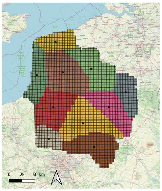
Figure 3.
Decomposition of the Hauts-de-France region in 10 zones for the selection of traffic and industrial layers by KNN with respect to the meteorological variables. The centroids of each zone are represented with black dots.
Note that, when predicting for time , a time is identified for each zone. A regional map of the traffic (respectively, industrial) layer is then reconstructed by projecting the zonal traffic (resp. industrial) maps onto a common 25 m resolution grid before combining them as follows:
Definition of the Calendar and Meteorological Parameters
The aforementioned calendar and meteorological parameters defining the coordinates of a couple of traffic and industrial layers observed at some date t are given in the Table 1. Several transformations are applied to the variables:

Table 1.
List of the calendar and meteorological parameters characterizing every observation of the historical data used for the KNN prediction of traffic and industrial layers.
- 1.
- To avoid potential confusion associated to the fact that the wind direction (denoted ) varies between 0 and 360 degrees, which both define the same angle, we calculate two new variables to replace the wind angle, defined as and , respectively.
- 2.
- For the sake of simplification, the precipitation rate is categorized into three categories, namely “low”, “medium” and “high” to facilitate the KNN selection. The variable thus takes three values, 1 (for rates between 0 and mm·), 2 (for rates between and 2 mm·) and 3 (for rates above 2 mm·).
- 3.
- To ensure that the coordinates of historical data (the meteorological parameters registered in ADMS-Urban) are comparable with those of the targeted date (the meteorological parameters from WRF data) when computing the Euclidean distance in the KNN procedure, we apply a min-max normalization as follows:Ensuring that all variables lie between 0 and 1 also ensures that the same importance is given to each of them.
These transformed parameters are given in Table 2.
Table 2.
List of the additional transformed meteorological variables defined from the original ones in order to simplify the KNN prediction of traffic and industrial layers.
3. Results and Discussion
Current research on air quality forecasting lacks a simple model that effectively combines both spatial and temporal dependencies. Many existing methods focus on either spatial or temporal aspects, failing to account for the complex interactions between geographic locations and pollutant concentrations over time [20]. Additionally, current models struggle to generalize across diverse urban environments due to variations in city structures and pollutant sources. With the increasing demand for real-time air quality forecasting, there is a clear need for models capable of rapid and accurate implementation that can quickly respond to dynamic air quality changes, surpassing traditional forecasting approaches. In recent years, numerous research papers have highlighted the potential applicability of various advanced statistical, machine learning and artificial intelligence methods to improve the spatial and temporal prediction of different pollutants using diverse data sources. For instance, Wang et al. [8] developed a unified and flexible composite modeling framework to accurately predict the concentration of six major air pollutants (, , , NO, and CO) in Shanghai. Their approach integrates both air monitoring and satellite-based data at a daily resolution. Based on a spatiotemporal trend model and spatiotemporal residuals, this method successfully estimates the concentrations of the aforementioned pollutants in urban areas at a fine spatial resolution of 100 m. Nevertheless, the authors noted that their method has certain limitations, particularly regarding wind speed and wind direction, which are not taken into account. As a result, there may be some bias related to the diffusion of pollutants. We have reached the same conclusion regarding the AZUR method, developed by our colleagues from the ATMO-Sud association, and applied to our data [6]. The AZUR method is based on the assumption that the daily concentrations between two measurement sites depend on the ratio of their annual value and their rank in their respective distribution. Thus, the daily (or hourly) maps can be constructed from annual maps corrected with the real-time or predicted data from monitoring stations. Consequently, the method can be applied with success for forecasting, as long as the modeled area is well-represented by monitoring stations. Jacquinot et al. [6] successfully applied the AZUR method in the Sud Provence-Alpes-Côte d’Azur region of France, and it was reproduced in our region from 2021 to 2024. However, in our case, while the method performs well in representing background pollution, certain issues related to the traffic and the industrial sectors have been identified. Firstly, the Hauts-de-France region has numerous significant point industrial sources, which may increase meteorology-dependent variability. Additionally, the number of monitoring stations, particularly those focused on traffic, is relatively low, making it impossible to adequately correct the map.
3.1. Industrial Plume Modeling
Modeling industrial plumes is challenging due to the intricate interplay of atmospheric conditions, source characteristics, terrain complexity and pollutant chemical transformations. Meteorological factors such as variable wind speed, direction, temperature and atmospheric stability significantly influence pollutant dispersion, while small-scale turbulence and thermal effects add further unpredictability. Source-specific parameters, including emission rates, pollutant composition and the geometry of chimneys or vents, must be precisely characterized, as they shape the initial behavior of the plume. The complexity increases in environments with uneven terrain, such as hills or valleys, or urban areas with buildings, which disrupt the airflow and create recirculation zones. In addition, pollutants often undergo chemical and physical changes, such as reactions leading to secondary pollutants or particle growth, which complicate predictions. Modeling approaches like Gaussian models, computational fluid dynamics (CFD) or mesoscale methods each have limitations, whether in computational efficiency, accuracy or their ability to account for localized phenomena, making plume modeling both a technically demanding and resource-intensive task.
Figure 4 presents an example of hourly concentration maps, with a focus on the northern coast of the Hauts-de-France region, obtained on 2 May 2024, at 2 p.m. using the method we propose. The issue of flat plumes, which previously did not adequately account for prevailing meteorological conditions, has been successfully resolved. The example clearly demonstrates that the industrial plume follows the wind direction and speed, making it a reliable tool for assessing air quality near industrial sources.
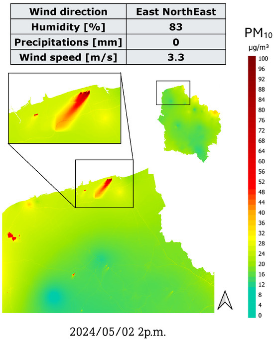
Figure 4.
Example of hourly concentration map over the northern part of the Hauts-de-France region (closer to cities of Calais and Dunkerque) for the targeted date of 2 May 2024 at 02:00 p.m. The meteorological data are provided on the top of the figure.
3.2. Temporal Variability in PM10 and NO2 Concentrations from Traffic Emissions
The temporal variability in and concentrations from traffic emissions is driven by a combination of emission patterns, meteorological conditions and atmospheric processes. Traffic emissions fluctuate throughout the day, with peaks typically coinciding with rush hours due to increased vehicle activity. Meteorological factors, such as wind speed and direction, atmospheric stability and temperature, further influence the dispersion and accumulation of pollutants, leading to variations between daytime and nighttime levels. Additionally, concentrations are affected by chemical reactions, such as the oxidation of NO emitted from vehicles, which depends on the availability of ozone and sunlight [21]. Seasonal differences also play a role, as lower temperatures and more stable atmospheric conditions in winter can lead to higher pollutant concentrations, while increased mixing in summer tends to disperse emissions more effectively. This dynamic interplay of factors results in a highly variable temporal pattern for and concentrations. There remains a significant need for precise estimation of spatial and temporal variations in air pollution. For example, Van den Hooven et al. [22] have highlighted the importance of examining the effects of exposure to both short- and long-term air pollution on various maternal and childhood outcomes, as well as identifying potential critical windows of exposure.
Figure 5 displays an example of concentration maps (sum of all contributions) close to an area where traffic emissions are high, at several hours of a specific day for . It can be observed that the KNN captures the traffic variability, with higher pollution levels during the day, especially in the beginning of the afternoon. This stays in agreement with other studies that have shown similar diurnal cycles of air pollutant concentrations. For instance, Krecl et al. [23] have shown that , NOx and CO show generally consistent pattern, peaking twice on weekdays and Saturdays (08:00 a.m.–10:00 a.m. and 06:00 p.m.–08:00 p.m.), which is typical of traffic environments.
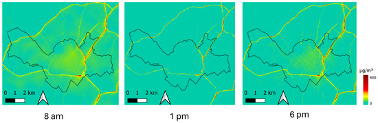
Figure 5.
Total concentration maps (background + industrial and traffic layers) at different hours of the date of 14 February 2025, in the area of Lille city in the Hauts-de-France region.
Figure 6 shows an example of time series of concentration extracted for the month of August 2024 at a monitoring station close to a road, that usually measures concentration values influenced by traffic emissions. The concentration time series extracted from the concentration map obtained after adding the KNN layers to the background layer is compared to the time series obtained from the background layer only. We observe that the KNN reconstruction exhibits a regular pattern with concentration peaks every day, whereas the background layer alone does not contain the information about the daily traffic-related concentration periodicity. This is expected because only background measures were used to construct the background layer, yet the periodicity of the KNN reconstruction shows a satisfying degree of realism.
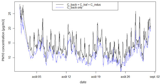
Figure 6.
Time series of concentration extracted close to a high traffic road in Beauvais (Hauts-de-France) from 1 to 31 August 2024, comparing the total concentration obtained with the KNN method with the background only.
3.3. High-Resolution Pollution Mapping
Hourly or daily pollution mapping provides high-resolution insights into the spatial and temporal distribution of air pollutants, enabling the identification of short-term patterns and hotspots. Urban air pollutant concentrations can vary significantly over short distances due to unevenly distributed emission sources and the dilution and transformation of pollutants. This fine-scale variation (10 m to 1 km) is crucial for understanding atmospheric chemistry, exposure assessment and environmental health. It also has societal implications, as urban planning, public health and environmental policies aim to address the often inequitable distribution of air pollution exposure [24].
Metamodels in air quality are simplified models designed to approximate the behavior of complex air quality models, offering a more computationally efficient alternative to resource-intensive simulations. Traditional air quality models, such as CFD or CTM, can be slow and costly to run, especially when evaluating multiple scenarios or optimizing pollution control measures across large areas. This becomes a significant problem for policymakers, urban planners and environmental researchers who need to make quick and informed decisions based on air quality predictions [25], as well as for citizens who require almost real-time information, hour by hour, to adapt their activities accordingly. Metamodels address this issue by enabling rapid scenario analysis, uncertainty quantification and high-resolution exposure assessments without computational burden. They use techniques such as statistical regression, machine learning, surrogate modeling or emulators such as Gaussian processes and neural networks to predict pollutant concentrations based on inputs such as emissions and meteorological data. Although metamodels are invaluable for tasks like policy evaluation and exposure mapping, their accuracy depends on the quality of the training data and their ability to generalize across different regions or scenarios. Despite these limitations, metamodels are increasingly being adopted in air quality research due to their ability to strike a balance between efficiency and precision [26].
In the present study, we used a KNN strategy, assuming that it can be an effective tool for metamodeling in air quality applications. KNN is a machine learning algorithm that predicts pollutant concentrations based on the nearest data points in a feature space, making it suitable for approximating complex air quality models. Using training data, including inputs such as meteorological conditions and emission rates, the KNN algorithm can predict pollutant levels for new scenarios. The method is non-parametric, meaning it does not assume a specific functional relationship between inputs and outputs, which is useful for capturing the complex, non-linear dynamics typical of air quality models. The simplicity of the KNN and ability to model local patterns make it an attractive option for tasks like exposure mapping and scenario analysis. KNN has already been used in air quality research due to its flexibility and ability to balance efficiency with predictive power. For instance, Chaeo et al. [11] developed a fuzzy evaluation approach to assess air pollution, combining an improved evidence theory, comprehensive weighting and the K-nearest neighbor interval distance within the matter–element extension model. The method demonstrated superior performance in capturing spatiotemporal variations and pollutant concentrations, reducing error rates by 38% compared to existing approaches. Other authors used the KNN for prediction of air quality index. Baran et al. [12] predicted Air Quality Index (AQI) values using Artificial Neural Networks (ANNs) and KNN algorithms. These predictions were based on key parameters, including , , CO, , temperature, humidity, pressure and wind speed. Similarly, in our case, the obtained results are interesting not only from the perspective of the quality of the provided information but also in terms of computational time, which could have been significantly optimized. Figure 7 displays an example of a regional hourly concentration map obtained by augmenting the background concentration map—obtained with the AZUR method—with the traffic and industrial KNN contributions.
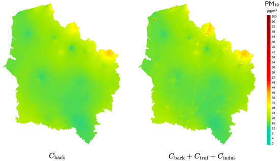
Figure 7.
Example of hourly concentration map computed over the Hauts-de-France region for the targeted date of 4 February 2025 at 11:00 a.m., with (right) and without (left) traffic and industrial layers.
3.4. Evaluation
In order to quantitatively validate our method, we carried out an evaluation of the KNN output using real pollutant measurements at the stations. This allowed for a quantitative evaluation of the ability of our method to accurately predict hourly concentration levels across the region. Two pollutants were considered in the present evaluation, namely and .
A first global evaluation was carried out using the KNN hourly output maps between 6 January and 13 March 2025, from which we extracted hourly predicted concentration data at the locations of the stations and compared them with the measurements. The available measurements of the stations and on this period are categorized depending on the influence of their measurements. Indeed, a measurement can be influenced by traffic or industrial emissions sources in which case we can categorize them as traffic measurements and industrial measurements. When it is not under such influence, it is said to be a background measurement. We compute statistical scores, namely linear bias, root mean squared error (RMSE) and Pearson linear correlation coefficient using samples of predictions and measurements, either combining all measurement influences (background, traffic and industrial) or isolating each type of influence. The results of this first evaluation are displayed in Table 3 with the corresponding sample sizes and number of available stations for each influence dataset.
Table 3.
Statistical scores computed comparing hourly KNN outputs with measurements from 6 January–13 March 2025, using different sets of stations depending on the influence of the corresponding measures—traffic, industrial and background. “Sample size” refers to the size of the data sample gathering all hours and stations available for a given influence and is the corresponding number of stations with available data.
From the statistical scores, we can understand that the model performs better on predictions than on predictions, and that there is a drop in accuracy when considering only stations at which the measurements are influenced by industrial and traffic sources. This is related to the fact that there are very few stations at which we have industrial and/or traffic measurements to compare with (only three stations for industrial measurements and four for traffic measurements, for instance). The prediction of seems to be damaged when isolating traffic measures because this pollutant has very localized dynamics and is thus more difficult to predict at an hourly fine-scale. The scores for when considering only industrial measurements happen to be better than those obtained with all measurements or only background measurements, which could come from the fact that, in proportion, most of the industrial measurements are collected when there is no large plume over the stations under industrial influence. A similar conclusion holds for industrial measurements, for which the scores are comparable to those obtained with all measures, and might be due to the fact that is mostly emitted by traffic and not industrial sources. Overall, the accuracy of our model on this two-month period is satisfactory, with correlations above 60% for measurements on all stations and on background stations only, and above 70% for .
A second evaluation was carried out using only traffic concentration measurements at a specific monitoring station in the city of Valenciennes, France. The KNN outputs were extracted at the station and we computed annual averages of predicted and measured hourly concentration values for both pollutants. Results are shown in Figure 8.
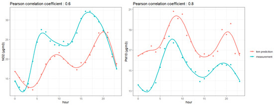
Figure 8.
Comparison of KNN predictions with measures at a traffic station in the city of Valenciennes in the Hauts-de-France region for (left) and (right). The dots represent yearly averaged values for each hour of the day, and the solid lines represent trends obtained with smoothing cubic spline functions.
As shown in the figure above, the concentration values obtained with our model are underestimating concentrations and overestimating concentrations, although with good correlations—the Pearson linear correlation coefficient is about 0.6 for and 0.8 for . Our predictions, evaluated on annual hourly averages retrieve the two daily peaks of measured concentrations in the morning and the evening, corresponding to traffic peak hours. This highlights the ability of our approach to capture the yearly-averaged daily concentration trends associated to traffic emissions The systematic bias between the annual hourly KNN prediction and reference measurements could come from the fact that the KNN estimate is chosen by minimizing a Euclidean distance in the space of calendar and meteorological parameters, but there is no guarantee that the hour and day of the selected traffic layer in the historical sample exactly match those of the targeted date. This could be improved by constraining the KNN algorithm to select layers in the historical data sample that correspond to the same hour and weekday as the targeted date. This could, however, demand a larger historical dataset. Moreover, the accuracy of this dataset could be improved by refining the ADMS-Urban simulations to better capture traffic concentrations (for example, by improving the temporal representation of traffic emissions).
Results from this evaluation study show the potential and limits of the method. Note that many factors can influence the performance of the model, such as the choice of the parameters, the uncertainty from the estimation of the background layer or the capacity of ADMS-Urban to estimate high concentration levels during high pollution periods. Despite the limited accuracy of the estimates at the stations where measures are influenced by traffic sources, our approach provides an efficient technique to capture the pollutant concentrations variability over time and to produce regional maps with satisfying global accuracy.
4. Conclusions
In the present research, we used a KNN-based strategy to predict air pollution levels based on real-time data from monitoring stations, meteorological variables (e.g., temperature, wind speed) and emission data. By applying the KNN approach to estimate traffic and industrial contributions, we were able to generate high-resolution air quality maps, providing pollutant concentration estimates at un-monitored locations. However, the method has certain limitations that could be addressed to improve its accuracy and applicability. Expanding the historical dataset could provide greater diversity in ADMS-Urban outputs, potentially enhancing precision. To overcome these limitations, future work could also focus on integrating real-time data from additional air quality monitoring stations and sensors to refine the model accuracy. One promising direction is the integration of data from so-called microsensors, which, while more cost-effective than traditional monitoring stations, present challenges related to a lower accuracy. Optimizing data assimilation techniques seems essential to ensure a seamless and reliable integration of these data sources into the modeling framework. Furthermore, to enhance the assessment of traffic-related emissions, we are exploring the incorporation of data from automatic vehicle counting stations. By combining real-time traffic flow data with air quality measurements, this approach could significantly improve the spatial resolution and reliability of traffic emission estimates, contributing to a more precise representation of urban air pollution dynamics. By using the KNN method, we have significantly reduced the computational time compared to the ADMS-Urban model while maintaining reliable results. The computational time was divided by 100, and using the traditional method would have required six servers instead of one. ADMS-Urban relies on complex numerical calculations and differential equations to simulate pollutant dispersion, requiring high computational power and long processing times, especially for high spatial and temporal resolutions. In contrast, KNN, with its instance-based learning approach, performs faster predictions by leveraging pre-computed data and efficient search structures like KD-trees or Ball-trees. This optimization reduces the time complexity and allows for rapid decision-making. While ADMS-Urban provides detailed physical modeling, KNN offers a faster alternative for applications where real-time or near-real-time predictions are essential. By choosing KNN, we have not only improved computational efficiency but also achieved significant energy savings, making it a practical choice for large-scale or time-sensitive analyses.
Author Contributions
Conceptualization, A.R. and N.P.-S.; methodology, L.B., A.R. and M.P.; validation, N.P.-S. and B.R.; writing—original draft preparation, L.B., A.R. and M.P.; writing—review and editing, H.C., N.P.-S. and B.R.; visualization, L.B., A.R. and M.P.; supervision, N.P.-S. and B.R. All authors have read and agreed to the published version of the manuscript.
Funding
This research was funded by Region Hauts-de-France and Agence Régionale de Santé Hauts-de-France.
Data Availability Statement
The data presented in this study are available upon request from the corresponding author due to privacy reasons.
Acknowledgments
We would like to thank François Legland for sharing his ideas, opinions and knowledge with us, which indirectly led to the creation of this article.
Conflicts of Interest
The authors declare no conflicts of interest.
Abbreviations
The following abbreviations are used in this manuscript:
| ADMS | Atmospheric Dispersion Modeling System |
| CERC | Cambridge Environmental Research Consultants |
| CFD | computational fluid dynamics |
| CTM | chemical transport models |
| HDF | Hauts-de-France |
| KNNs | k-nearest neighbors |
| particulate matter of size less than 10 μm | |
| particulate matter of size less than 2.5 μm | |
| RMSE | root mean squared error |
| WRF | Weather Research Forecast |
References
- Directive (EU) 2024/2881; Ambient Air Quality and Cleaner Air for Europe (Recast). European Parliament, Council of the European Union: Brussels, Belgium, 2024.
- Patel, Z.B.; Purohit, P.; Patel, H.M.; Sahni, S.; Batra, N. Accurate and Scalable Gaussian Processes for Fine-Grained Air Quality Inference. Proc. AAAI Conf. Artif. Intell. 2022, 36, 12080–12088. [Google Scholar] [CrossRef]
- Casallas, A.; Cabrera, A.; Guevara-Luna, M.A.; Tompkins, A.; González, Y.; Aranda, J.; Belalcazar, L.C.; Mogollon-Sotelo, C.; Celis, N.; Lopez-Barrera, E.; et al. Air pollution analysis in Northwestern South America: A new Lagrangian framework. Sci. Total Environ. 2024, 906, 167350. [Google Scholar] [CrossRef]
- William, R. Stockwell, Emily Saunders, W.S.G.; Fitzgerald, R.M. A perspective on the development of gas-phase chemical mechanisms for Eulerian air quality models. J. Air Waste Manag. Assoc. 2020, 70, 44–70. [Google Scholar] [CrossRef]
- Menut, L.; Cholakian, A.; Pennel, R.; Siour, G.; Mailler, S.; Valari, M.; Lugon, L.; Meurdesoif, Y. The CHIMERE chemistry-transport model v2023r1. Geosci. Model Dev. Discuss. 2024, 17, 5431–5457. [Google Scholar] [CrossRef]
- Jacquinot, M.; Derain, R.; Armengaud, A.; Oppo, S. Spatial model for daily air quality high resolution estimation. Air Qual. Atmos. Health 2024, 17, 2141–2150. [Google Scholar] [CrossRef]
- Badawy, H. Recent trends in spatial modeling studies of air quality (2010–2023). Earth Sci. Inform. 2025, 18, 193. [Google Scholar] [CrossRef]
- Wang, Y.; Huang, L.; Huang, C.; Hu, J.; Wang, M. High-resolution modeling for criteria air pollutants and the associated air quality index in a metropolitan city. Environ. Int. 2023, 172, 107752. [Google Scholar] [CrossRef]
- Rybarczyk, Y.; Zalakeviciute, R. Machine Learning Approaches for Outdoor Air Quality Modelling: A Systematic Review. Appl. Sci. 2018, 8, 2570. [Google Scholar] [CrossRef]
- Tang, D.; Zhan, Y.; Yang, F. A review of machine learning for modeling air quality: Overlooked but important issues. Atmos. Res. 2024, 300, 107261. [Google Scholar] [CrossRef]
- Chao, B.; Guang Qiu, H. Air pollution concentration fuzzy evaluation based on evidence theory and the K-nearest neighbor algorithm. Front. Environ. Sci. 2024, 12, 1243962. [Google Scholar] [CrossRef]
- Baran, B. Air Quality Index Prediction in Besiktas District by Artificial Neural Networks and K Nearest Neighbors. MüHendislik Bilim. Ve Tasarım Derg. 2021, 9, 52–63. [Google Scholar] [CrossRef]
- Atmo Sud. Why Do We Need to Change the Air Quality Information Indexes to a HD Mapping Approach? Technical Report; Atmo Sud: Marseille, France, 2024. [Google Scholar]
- Carruthers, D.J.; Edmunds, H.A.; McHugh, C.A.; Singles, R.J. Development of Adms-Urban and Comparison with Data for Urban Areas in the UK. In Air Pollution Modeling and Its Application XII; Springer: Boston, MA, USA, 1998; pp. 467–475. [Google Scholar] [CrossRef]
- Stocker, J.; Hood, C.; Carruthers, D.; Mchugh, C. ADMS-Urban: Developments in modelling dispersion from the city scale to the local scale. Int. J. Environ. Pollut. 2012, 50, 308–316. [Google Scholar] [CrossRef]
- Snoun, H.; Krichen, M.; Chérif, H. A comprehensive review of Gaussian atmospheric dispersion models: Current usage and future perspectives. Euro-Mediterr. J. Environ. Integr. 2023, 8, 219–242. [Google Scholar] [CrossRef]
- Beauchamp, M.; de Fouquet, C.; Malherbe, L. Dealing with non-stationarity through explanatory variables in kriging-based air quality maps. Spat. Stat. 2017, 22, 18–46. [Google Scholar] [CrossRef]
- Babak, O.; Deutsch, C. Statistical approach to inverse distance interpolation. Stoch. Environ. Res. Risk Assess. 2008, 23, 543–553. [Google Scholar] [CrossRef]
- Cover, T.; Hart, P. Nearest neighbor pattern classification. IEEE Trans. Inf. Theory 1967, 13, 21–27. [Google Scholar] [CrossRef]
- Jayaraman, S. Enhancing urban air quality prediction using time-based-spatial forecasting framework. Sci. Rep. 2025, 15, 4139. [Google Scholar] [CrossRef]
- Liu, M.; Lin, J.; Wang, Y.; Sun, Y.; Zheng, B.; Shao, J.; Chen, L.; Zheng, Y.; Chen, J.; Fu, T.M.; et al. Spatiotemporal variability of NO2 and PM2.5 over Eastern China: Observational and model analyses with a novel statistical method. Atmos. Chem. Phys. 2018, 18, 12933–12952. [Google Scholar] [CrossRef]
- Van den Hooven, E.H.; Pierik, F.H.; Van Ratingen, S.W.; Zandveld, P.Y.; Meijer, E.W.; Hofman, A.; Miedema, H.M.; Jaddoe, V.W.; De Kluizenaar, Y. Air pollution exposure estimation using dispersion modelling and continuous monitoring data in a prospective birth cohort study in the Netherlands. Environ. Health 2012, 11, 9. [Google Scholar] [CrossRef]
- Krecl, P.; Castro, L.B.; Targino, A.C.; Oukawa, G.Y. Spatio-temporal variability and trends of air pollutants in the Metropolitan Area of Curitiba. Heliyon 2024, 10, e40651. [Google Scholar] [CrossRef]
- Apte, J.S.; Manchanda, C. High-resolution urban air pollution mapping. Science 2024, 385, 380–385. [Google Scholar] [CrossRef] [PubMed]
- Hammond, J.K.; Chen, R.; Mallet, V. Meta-modeling of a simulation chain for urban air quality. Adv. Model. Simul. Eng. Sci. 2020, 7, 37. [Google Scholar] [CrossRef]
- Pisoni, E.; De Marchi, D.; di Taranto, A.; Bessagnet, B.; Sajani, S.Z.; De Meij, A.; Thunis, P. SHERPA-Cloud: An open-source online model to simulate air quality management policies in Europe. Environ. Model. Softw. 2024, 176, 106031. [Google Scholar] [CrossRef]
Disclaimer/Publisher’s Note: The statements, opinions and data contained in all publications are solely those of the individual author(s) and contributor(s) and not of MDPI and/or the editor(s). MDPI and/or the editor(s) disclaim responsibility for any injury to people or property resulting from any ideas, methods, instructions or products referred to in the content. |
© 2025 by the authors. Licensee MDPI, Basel, Switzerland. This article is an open access article distributed under the terms and conditions of the Creative Commons Attribution (CC BY) license (https://creativecommons.org/licenses/by/4.0/).