Article

A Hybrid Transformer-CNN Model for Interpolating Meteorological Data on the Tibetan Plateau

1
School of Atmospheric Physics, Nanjing University of Information Science & Technology, Nanjing 210044, China
2
Institute of Atmospheric Physics, Chinese Academy of Sciences, Beijing 100029, China
3
MeteoNex Technology Co., Ltd., Xiongan 071800, China
*
Author to whom correspondence should be addressed.
Atmosphere 2025, 16(4), 431; https://doi.org/10.3390/atmos16040431
Submission received: 10 March 2025 / Revised: 30 March 2025 / Accepted: 2 April 2025 / Published: 8 April 2025
(This article belongs to the Section Atmospheric Techniques, Instruments, and Modeling)

Abstract

:
High-quality observational data play a crucial role in deepening the investigation of the Tibetan Plateau’s influence on the Asian climate. This study employs eight machine learning models (support vector regression (SVR), k-nearest neighbors (KNN), extreme gradient boosting (XGBoost), random forest (RF), long short-term memory (LSTM), gated recurrent unit (GRU), Transformer, and Transformer–convolutional neural network (Transformer-CNN)) to interpolate missing observational data on surface net radiation (Rn), soil surface temperature (Ts), soil water content (SWC), air temperature (Ta), relative humidity (RH), and wind speed (WS) from the QOMS observation site. The data covers the period from 1 January 2007 through to 31 December 2016. A comparative evaluation of these models shows that the Transformer-CNN model consistently outperforms the other models in terms of prediction accuracy. On the test dataset, the coefficients of determination for the interpolated results of Ta, RH, WS, SWC, Ts, and Rn were 0.97, 0.92, 0.97, 0.79, 0.93, and 0.98, respectively. Secondly, the Transformer-CNN model was then applied to generate a complete meteorological dataset for the full period. A time series analysis of this dataset reveals statistically significant trends over the past decade: air temperature (Ta) increased by 0.60 °C (p = 0.022) and soil temperature (Ts) by 1.85 °C (p = 1.37 × 10⁵). Meanwhile, wind speed (WS), soil water content (SWC), and net radiation (Rn) declined by 0.42 m/s (p = 1.18 × 10¹²), 1.24% (p < 0.001), and 9.21 W/m2 (p = 8.81 × 10⁶), respectively.

1. Introduction

The Tibetan Plateau, known as the “Roof of the World,” covers an area of approximately 2.5 million square kilometers and is the highest and most extensive plateau globally [1,2]. Studies have shown that it is one of the most sensitive regions to global warming, with its climate changes significantly impacting global climate patterns [3]. High-quality meteorological data are fundamental for meteorological analysis and understanding climate dynamics [4]. However, due to technical, human, and natural factors, meteorological data are often missing, especially in remote and harsh environments like the Tibetan Plateau [5]. These data gaps hinder the accurate identification of climatic changes and trends, thereby affecting the validity of climate research in this critical region. Given the Plateau’s significant role in global climate patterns, addressing these data deficiencies is particularly important. Accurate and effective interpolation methods help maintain the continuity of time series data, allowing for a more comprehensive utilization of available observational data in scientific research [6]. This facilitates a better understanding and prediction of climate changes in the region [7]. Therefore, the development of effective interpolation methods is crucial for overcoming these challenges and ensuring the continuity and accuracy of meteorological data [8,9,10,11].
Common interpolation methods for meteorological data can be broadly categorized into spatial interpolation, temporal interpolation, statistical interpolation, and hybrid interpolation. In spatial interpolation, Yu et al. [12] utilized the standard sequence method for interpolating daily average temperatures, finding that selecting neighboring stations based on the “best correlation” yielded better results than using the “closest distance” criterion. In temporal interpolation, Li et al. [13] introduced a reverse-order interpolation method based on conventional sequential interpolation, achieving higher accuracy in filling missing data segments. Sun et al. [14] compared inverse distance weighting, ordinary Kriging, and multiple linear regression methods in the temporal interpolation of daily average, maximum, and minimum temperatures in Hubei Province. They discovered that multiple linear regression was the most effective for filling missing daily temperature data, making it suitable for establishing long-term continuous temperature datasets at meteorological stations. For statistical and hybrid interpolation methods, early work by Gandin and Kagan laid the foundation for optimum interpolation techniques based on correlation analysis [15]. Subsequent studies have shown [16] that arithmetic mean, multiple linear regression, and nonlinear iterative partial least squares methods perform best in filling missing precipitation data. Among these, the multiple regression method successfully estimated missing precipitation data, while multiple imputation methods produced the most accurate results. Additionally, other studies [17] have employed similarity interpolation, two-step interpolation, and hybrid methods that integrate spatial, temporal, and similarity interpolations to minimize errors.
While traditional interpolation techniques have provided valuable solutions for addressing missing meteorological data, they often struggle with capturing complex patterns in large datasets [18,19]. Recent advances in computational power and machine learning algorithms have opened new avenues for more accurate and efficient data interpolation [20,2122]. Advances in neural network technologies have made it possible to efficiently process large-scale meteorological data, leading to their gradual application in meteorological data interpolation research [23]. Han et al. [24] used reanalysis gridded data to interpolate abnormal wind tower data using methods such as equal-weight averaging, weighted averaging, optimal nearest grid point, bilinear interpolation, inverse distance weighting, and artificial neural network (ANN) interpolation. The results showed that backpropagation (BP) neural network interpolation provided the best fit among these methods. Combining rough set theory with radial basis function (RBF) neural networks. Tang et al. [25] established a model for interpolating missing data, which more effectively and accurately interpolated single-station meteorological data than general linear interpolation methods. Zheng et al. [26] managed to precisely interpolate missing half-hour temperature observation data by employing a sequence-to-sequence deep learning structure (BiLSTM-I) based on an encoder–decoder architecture. The results indicated that the BiLSTM-I deep learning method outperformed other methods, meeting the needs for high-precision interpolation of temperature data. Mital et al. [27] proposed filling missing precipitation data based on random forest technology, which showed excellent performance, and thus could also be applicable to other meteorological elements.
Deep learning models like the Transformer and convolutional neural networks (CNN) have shown remarkable performance in handling time series data, making them ideal for processing the complex meteorological data from the Tibetan Plateau [28,29]. The Transformer model, proposed by Google in 2017 [30], incorporates a self-attention mechanism that effectively captures long-term dependencies in time series data. This is particularly beneficial for meteorological datasets from the Tibetan Plateau, where environmental factors create intricate temporal patterns. CNNs, which have been successfully applied to time series analysis and prediction, are adept at recognizing patterns over varying time scales, capturing the periodic variations in meteorological elements. The newly developed Transformer-CNN model combines these two approaches: CNN captures the periodic characteristics at different time scales, while the Transformer captures long-distance dependencies [31]. This combination allows for a more accurate representation of the complex variation patterns in meteorological data influenced by environmental elements. Given the unique geographical and climatic conditions of the Tibetan Plateau, traditional methods often struggle to model these complexities. Therefore, employing advanced deep learning models like the Transformer and CNN is particularly suitable for addressing the challenges in this region. However, the application of deep learning in meteorological data analysis for the Tibetan Plateau is still in its infancy, with relatively little research utilizing these advanced models in this context.
In order to obtain a complete meteorological dataset for the QOMS station from 2007 to 2016, so as to provide a powerful tool for assessing climate on the Tibetan Plateau, this study aims to explore the feasibility of using the Transformer-CNN model to interpolate key meteorological elements collected at the QOMS station during the Third Tibetan Plateau Scientific Expedition from 1 January 2007 to 31 December 2016. These elements include surface net radiation (Rn), soil temperature (Ts), surface soil water content (SWC), air temperature (Ta), relative humidity (RH), and wind speed (WS). Additionally, we will quantitatively evaluate the accuracy of the Transformer-CNN model by comparing its performance with other artificial intelligence models in interpolating these elements.

2. Materials and Methods
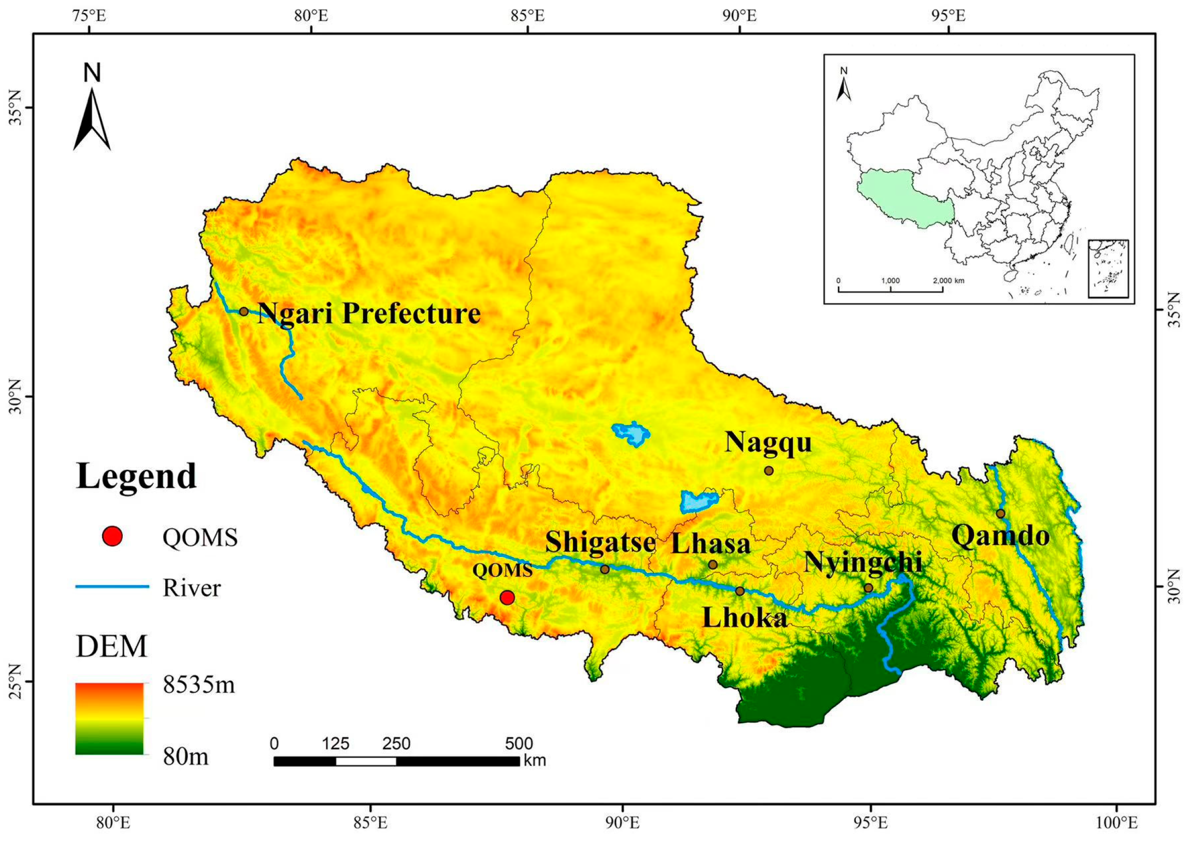
2.1. Study Area

The data used in this study were sourced from the QOMS station (28.36° N, 86.95° E) located on the northern slope of the Tibetan Plateau, as shown in Figure 1. The observation site is situated at the Ruobula Pass, with the surface covered by gravel and sparse vegetation [32], as it is able to provide extensive coverage for monitoring heterogeneous mountainous environments and climates, thus aiding in the evaluation and improvement of artificial intelligence models.

2.2. Data

The observational data collected from the QOMS site for the period from 1 January 2007 to 31 December 2016 were analyzed using the elements including sensible heat flux (H), latent heat flux (LE), soil heat flux (G0), wind direction at five levels (Wd), surface net radiation (Rn), surface temperature (Ts), and surface soil volumetric water content (SWC) collected at the site, as well as air temperature (Ta), relative humidity (RH) and wind speed collected 1.5 m above the site. Details of the observed variables and the corresponding instruments are provided in Table 1. The observational data used in this study are at an hourly frequency.
The time series data for air temperature, relative humidity, wind speed, air pressure, soil temperature, soil moisture, and net radiation were also subjected to quality control. Using a four standard deviation threshold to identify and remove noise may lead to fewer data points being discarded as outliers, thereby reducing the overall missing data rate. In the unique high-altitude climate conditions of the QOMS station, this approach not only enhances dataset integrity but also mitigates the uncertainty introduced into subsequent interpolation models by excessively high missing data rates [33]. Noise data were eliminated on the criteria X(h) < (X − 4σ) or X(h) > (X + 4σ), where X(h) represents component time series, X is the mean deviation during the interval, and σ is the standard deviation [34]. The missing rates of the meteorological elements after quality control are shown in Table 2.

2.3. Data Processing

To ensure the completeness of environment-driven elements when machine learning algorithms were used for flux data interpolation, the k-nearest neighbors(K-NN) interpolation method was employed in the data preprocessing stage to handle missing environment-driven elements [35]. KNN interpolation is a non-parametric method that does not require assumptions about the distribution of meteorological elements. It involves finding the nearest neighbor observations of missing values in the time dimension and using a “distance weighted” approach for interpolation. The local characteristics of this method ensure that interpolation relies only on local data similar to missing values. Data consistency is guaranteed, especially in environment-driven elements, where temporal proximity often indicates the similarity of elements [36]. Moreover, environmental driving elements such as temperature and humidity may have complex nonlinear relationships, and the KNN interpolation method can be directly applied without explicit model assumptions [37]. The number of neighbors was set to three, and “distance” was used for the weight calculation method to ensure that the closer the observations, the higher the weights [38]. The specific calculation formula is expressed as:
G a p f i l l i n g   v a l u e = i = 1 3 y i d i i = 1 3 i d i
where y i represents the observed value of the i-th nearest neighbor; di denotes the distance between the missing value and the i-th nearest neighbor; the summation in the numerator is the weighted sum of the observed values and the reciprocals of the distances of the three nearest neighbors; the summation in the denominator is the sum of the reciprocals of the distances of the three nearest neighbors.
Air temperature (Ta) was selected as the primary target element for interpolation in the present study as this dataset was the most complete. The remaining environment-driven elements were then interpolated using the K-NN method, which in turn drove the artificial intelligence model. Upon the completion of Ta interpolation, the complete Ta dataset was then used as an environment-driven element to interpolate the next target element, and this process was repeated iteratively. Ultimately, a complete meteorological element dataset at the QOMS site was obtained. In this study, the elements were interpolated in the order of Ta, RH, WS, SWC, Ts, and Rn based on their degree of completeness.

2.4. Experiments

This study aims to fit the missing values of basic meteorological elements using ten years of observational data collected from the QOMS meteorological station on the Tibetan Plateau, spanning from 2007 to 2016. By analyzing the interannual variations in basic meteorological elements and treating the missing parts as quantitative predictive elements, this study attempts to construct a complete dataset of basic meteorological elements.
Proper allocation of the training, validation, and test sets is crucial for the application of the model. The training set (2007–2012, 2014–2016) is used for learning patterns and structures in the data, the validation set (10% of the samples randomly drawn from the training set) for model selection and hyperparameter tuning, and the test set (2013 data) for independently evaluating the model’s performance on new data. The entire dataset used in this study comprises 87,673 samples, with approximately 80% used for training, 10% for validation, and the remaining 10% for test. This approach takes into account the complexity of time series analysis, ensuring rigorous model validation and testing, and providing a reliable method for interpolating meteorological elements at the station.

2.4.1. OOB (Out-of-Bag)

Out-of-bag (OOB) error is a method used in the random forest algorithm to estimate the model’s performance. It cannot be calculated merely by a separate test set or validation set. In the training process of a random forest, each tree is trained on a subset of the samples, while the samples not involved in training that particular tree (i.e., OOB samples) are used to evaluate the model’s performance, implying that the importance of features can be effectively assessed even with a limited amount of data [39].
Assuming N is the total number of samples, Oi is the out-of-bag prediction for the i-th sample, and y i is the actual value, the OOB error can be calculated by:
O B B s c o r e = 1 N i = 1 N L ( y i , O i )
where L is the loss function. In this study, the root mean square error (RMSE) was utilized as the loss function.
The importance of features was evaluated by observing the change in OOB error after the removal or alteration of a specific feature. In this case, a significant increase in OOB error indicates that the feature plays a significant role in the model’s performance.

2.4.2. Machine Learning Models

In the field of machine learning, various algorithms have been widely applied to data fitting and prediction. RF (random forest) [40] is employed by constructing multiple decision trees and iteratively uses existing variables to predict missing values if there are any. This algorithm performs well in high-dimensional spaces and is suitable for nonlinear relationships. SVR [41] can achieve excellent results when handling missing values under the premise that the relationships between data points can be effectively separated by a hyperplane. KNN [42] predicts missing values by finding the k-nearest neighbors based on a certain distance metric, where missing values are replaced by the average or majority vote of their k-nearest neighbors, but exhibits poor performance on large-scale datasets. XGBoost [43], a gradient boosting-based ensemble learning algorithm, addresses missing values by iteratively constructing decision trees while considering the direction of missing values at each step of selecting the split points.

2.4.3. Deep Learning Models

In the realm of data imputation, LSTMs [44] (long short-term memory networks), GRUs (gated recurrent units), and Transformer are commonly used deep learning methods. Among them, LSTM, a special type of recurrent neural network (RNN), is capable of learning long-term dependencies in sequence data. In data imputation, LSTM can be employed to learn patterns within a time series to predict or estimate missing values. GRU [45], a variant of RNN, is similar to LSTM but has a simpler structure. It controls the flow of information through reset and update gates, making it suitable for imputing time series data. The Transformer model [30] based on a self-attention mechanism, handles long-distance dependencies in sequence data, and it is also able to input and process the entire sequence in parallel, thereby effectively imputing missing values.

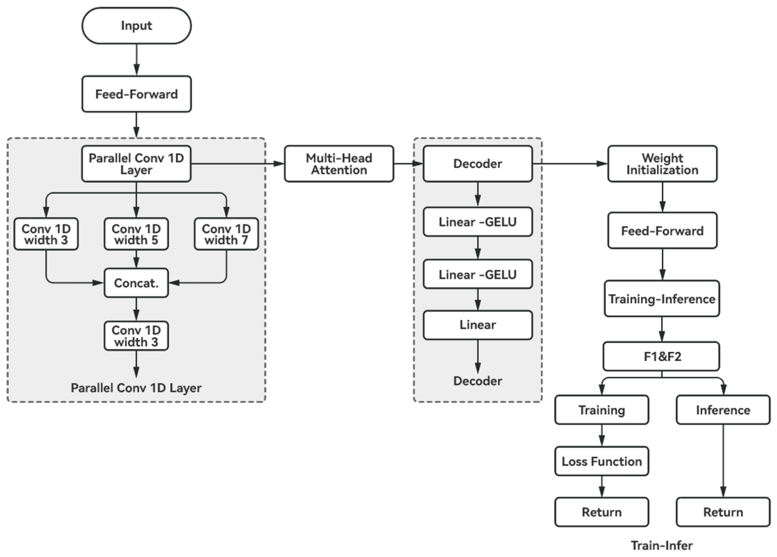
2.4.4. Transformer-CNN

In addressing the complexity of data from the Tibetan Plateau, this study employed a deep neural network model based on the PyTorch (version 1.15) framework (as shown in Figure 2), using environmental drivers as features and interpolated meteorological elements as targets to input into the model. In the initialization phase, a layer normalization component was integrated to normalize the input along the embedding dimension, enhancing the stability and convergence efficiency of the training process. The model consisted of a feedforward network comprising three fully connected layers that capture nonlinear features by integrating ReLU activation functions. Additionally, three one-dimensional convolutional layers with different kernel sizes were embedded into the model to extract local features across various time scales, such as the periodic variations in turbulent heat flux. Another one-dimensional convolutional layer was used to integrate the outputs of the aforementioned convolutional layers to form a comprehensive feature representation.
The model utilized a multi-head self-attention mechanism with four attention heads (multi-head attention component) to capture long-range dependencies within the input sequence. The encoded features in the decoder section were mapped to the target space. Furthermore, a weight initialization component was employed to scientifically initialize the weights and biases, thereby ensuring the stability of the model.
The forward propagation process of the model was defined by the feed-forward function. The model generated two data views during its application, namely F1 (primary view) and F2 (contrast view). Despite the application of dropout techniques, there were still potential differences between these two views. Smooth L1 loss served as the loss function, which was composed of three parts, namely the error between F1 and the true value, the error between F2 and the true value, and the distance between F1 and F2 as a regularization term, the latter multiplied by a coefficient of 0.1. In the interference phase, the final prediction results of the model were presented by averaging F1 and F2. This result is the final output value of the model, which is the interpolation value of the meteorological element by the model.
In summary, the model effectively addresses data complexity through the combination of layer normalization, a multilayer fully connected network, multi-scale convolutions, and a multi-head self-attention mechanism, ensuring its stability and efficacy. This structural design enables the model to comprehensively utilize various feature extraction and long-range dependency capture techniques to more accurately predict and analyze the complex environmental data of the Tibetan Plateau.

2.4.5. Assessment of Model Performance

Numerous model performance metrics were used in the subsequent assessment of model performance, including:
Root mean square error (RMSE): RMSE represents the square root of the mean value of the squared errors; that is, the average of the differences between the simulated and observed values. The lower the RMSE value, the better the model’s fit.
R M S E = 1 n   i = 1 n ( y i y ^ i ) 2  
Mean absolute error (MAE): MAE calculates the average of the absolute differences between the observed and predicted values. The lower the MAE value, the better the model’s fit.
M A E = 1 n i = 1 n | y i y ^ i |
Coefficient of determination (R2): coefficient of determination measures the proportion of the variance in the dependent variable that is predictable from the independent variables. This metric indicates how close the data are to the fitted regression line. The closer its value is to 1, the more effectively the model explains the variability of the data.
R 2 = 1 i = 1 n ( y i y ^ i ) 2 i = 1 n ( y i y ¯ i ) 2
where n is the total sample size, y i is the observed value, y ^ is the model predicted value, and y ¯ is the sample mean.

3. Results

3.1. Feature Importance and OOB Score

As show in Figure 3, a total of 12 feature factors were analyzed using the random forest method to evaluate their relative importance for different meteorological elements. Air temperature (Ta) and soil temperature (Ts) were both primarily influenced by each other, with soil temperature showing the highest importance for Ta, and vice versa, each exceeding 80% in importance. Relative humidity (RH) was most strongly associated with wind speed. Wind speed (WS) was mainly influenced by air humidity and pressure, which together accounted for over 50% of the total importance. For soil water content (SWC), precipitation was the dominant factor. Surface net radiation (Rn) showed the highest association with sensible heat flux, with an importance value exceeding 80%.
By calculating out-of-bag (OOB) scores under varying input feature dimensions and adding elements in descending order of their importance, we identified the optimal feature combinations for each target meteorological element. As shown in Figure 4, for air temperature (Ta), the highest OOB score was obtained by including the top ten features ranked by importance, and adding more than ten features did not yield further performance improvements. In contrast, for relative humidity (RH), wind speed (WS), and soil water content (SWC), the simulation performance continued to improve as additional environment-driven elements were introduced, resulting in all twelve analyzed features being selected as the optimal combination. Soil temperature (Ts) exhibited a more constrained set of influential factors, with the top six features delivering the best OOB score and no performance gains observed beyond the sixth feature. Similarly, surface net radiation (Rn) achieved peak predictive accuracy with the top nine features, and adding further factors did not enhance the model. Collectively, these findings demonstrate that optimal feature subsets vary across meteorological parameters, reflecting the distinct physical processes governing each element’s behavior.

3.2. Inter-Comparison

Table 3 presents a comparative analysis of the Transformer-CNN model and several other artificial intelligence models in the test dataset, using the coefficient of determination (R2) and root mean square error (RMSE) as evaluation metrics. The results show that Transformer-CNN exhibits clear advantages in long-term prediction, consistently achieving lower RMSE and higher R2 values compared to other models. It is apparent from the table that the Transformer model is superior to other single modes in terms of fitting performance, which, therefore, is selected as the framework for the hybrid model. Additionally, Transformer-CNN outperforms the traditional Transformer model in data fitting performance.
First, the incorporation of convolutional neural networks (CNN) enhances the model’s capability for local feature extraction. A CNN, through its convolutional layers, is able to capture significant seasonal and periodic variations in turbulent heat flux. By identifying these local patterns, CNN can recognize daily, monthly, and seasonal changes in turbulent flux, making it advantageous for capturing complex patterns in the data.
Second, predicting turbulent heat flux involves complex physical processes and multi-scale interactions. The Transformer model’s advantage in capturing long-distance dependencies, combined with CNN’s local feature extraction capability, enhances the model’s flexibility and diversity. Moreover, high convolutional operation efficiency may contribute to improved model training speed and efficiency. By integrating CNN and Transformer into a hybrid model, both local and global features can be simultaneously captured, demonstrating its adaptability in predicting missing data.

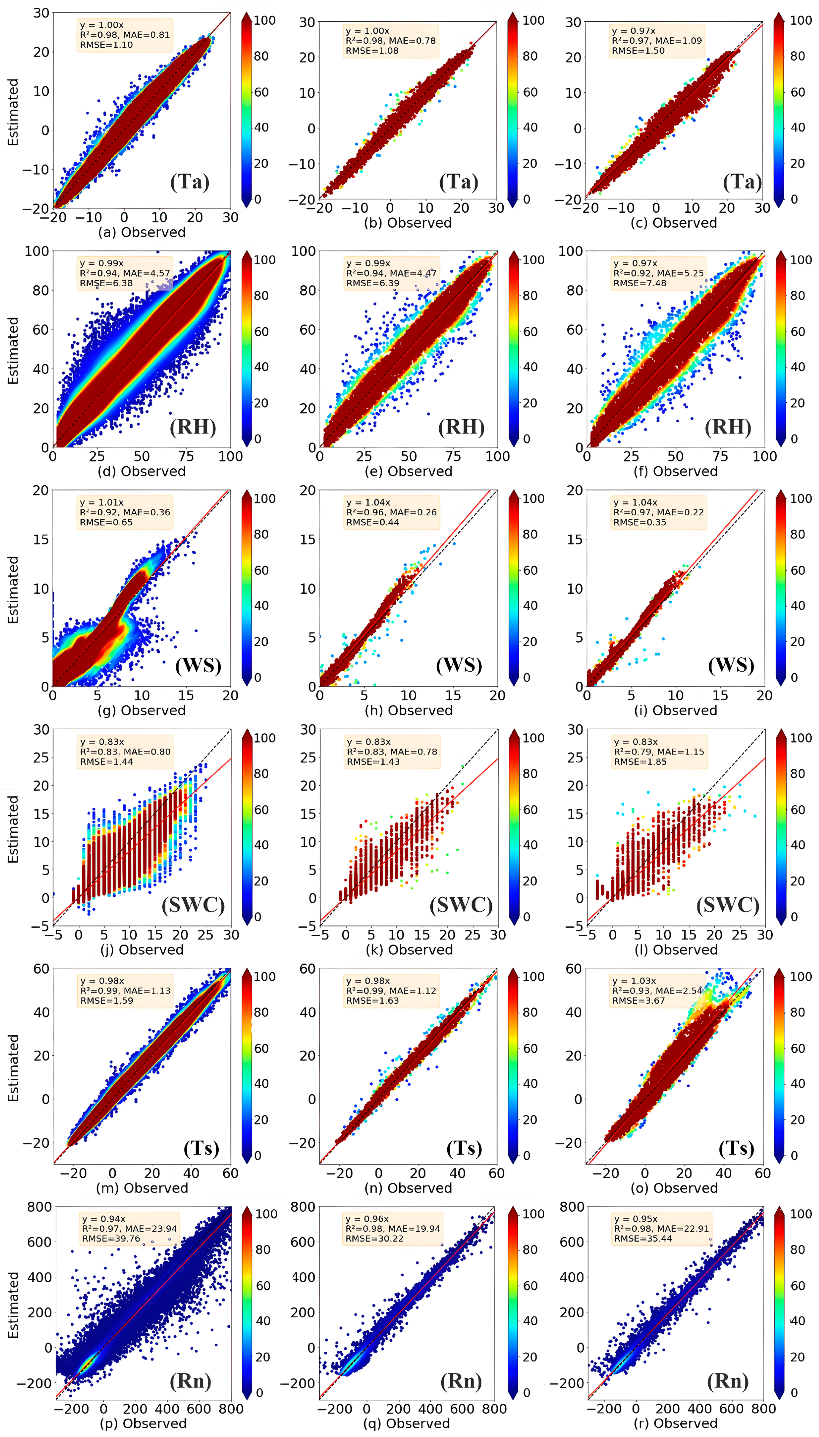
3.3. Scatter Plot of Transformer-CNN

Figure 5 presents scatter plots comparing the observed values with the actual values for each meteorological element. The intensity of the red coloration indicates the density of the data points, with deeper red hues representing higher concentrations. The solid line denotes the 1:1 identity line, while the dashed line represents the fitted regression curve. The distance between the data points and the identity line quantifies the prediction error. Across various meteorological elements, the Transformer-CNN model demonstrates robust predictive capabilities at the QOMS station on the Tibetan Plateau. For air temperature (Figure 5a–c), the predicted values closely match the actual measurements, with a near-unity curvature (y = 1.00x) and an R2 of 0.98 in training and validation, and an R2 of 0.97 in testing. Relative humidity (Figure 5d) also displays excellent agreement, achieving an R2 of 0.92 and low error metrics (MAE = 5.25, RMSE = 7.48), effectively capturing a broad distribution of humidity levels. Wind speed predictions exhibit similar success, with an R2 of 0.97 and slight systematic biases at low (WS ≤ 6) and high (WS ≥ 10) speeds. Although soil water content predictions (Figure 5k) slightly underestimate observed values due to the complexity of moisture dynamics, the model still obtains an R2 of 0.79 and acceptable error measures (MAE = 1.15, RMSE = 1.85). Soil temperature predictions (Figure 5o) are more accurate, with an R2 of 0.93, MAE of 2.54, and RMSE of 3.67, effectively capturing the thermal variations from −20 °C to 50 °C. Finally, for ground net radiation (Figure 5r), the model attains an R2 of 0.98 and relatively low error metrics (MAE = 22.91, RMSE = 35.44). Taken together, these results underscore the Transformer-CNN model’s strong performance and versatility in interpolating missing meteorological values across multiple elements.

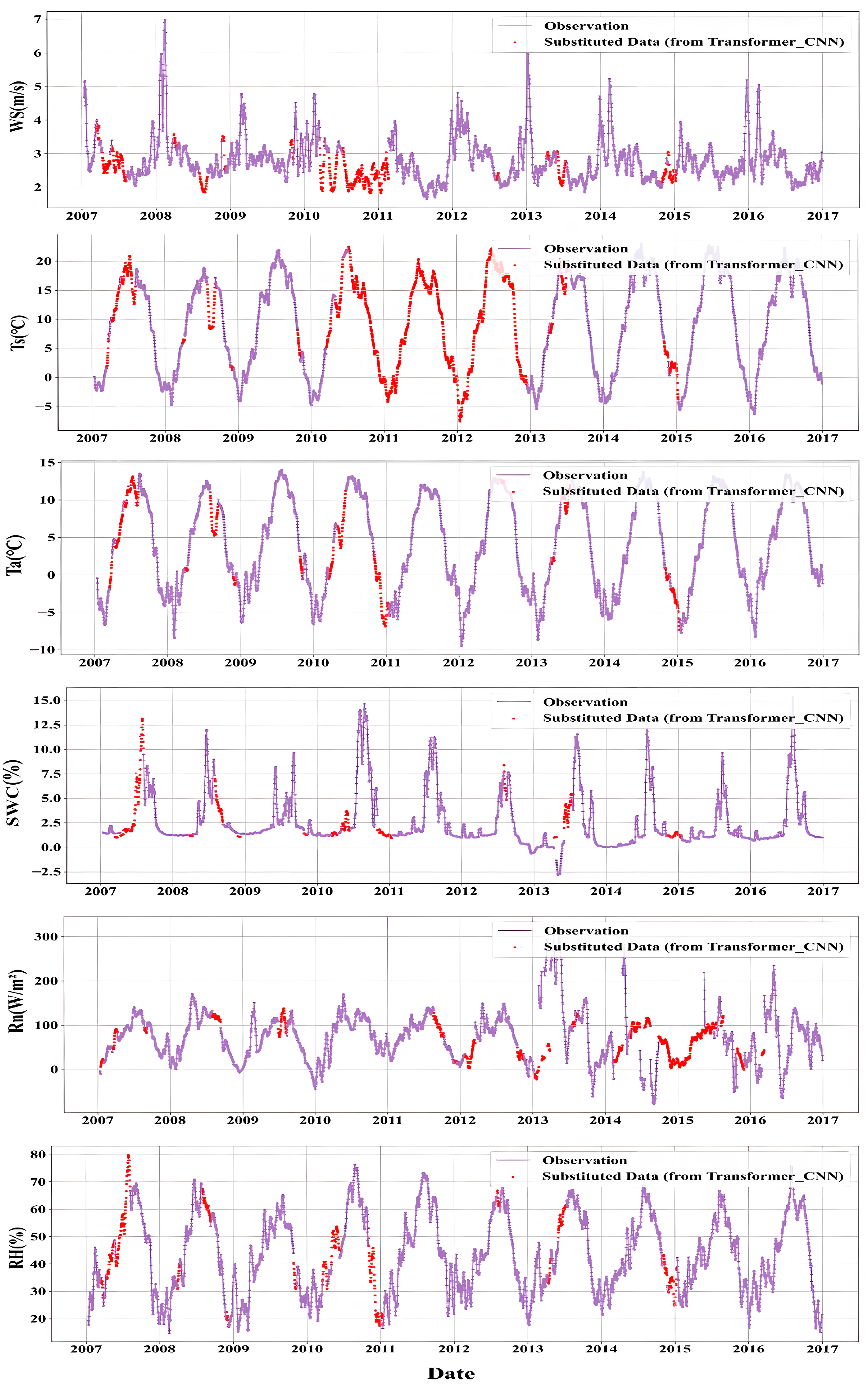
3.4. Complete Dataset

By utilizing the Transformer-CNN model to comprehensively impute the meteorological data of the QOMS site, we obtained a complete and continuous dataset of meteorological elements. As shown in Figure 6, the purple points represent the observed values, while the red points indicate the imputed values generated by the model. Over the ten-year analysis period at the QOMS station on the Tibetan Plateau, daily average variations in multiple meteorological elements, reconstructed through Transformer-CNN interpolation, reveal distinct seasonal patterns and strong consistency with observed data. For air temperature, pronounced seasonal differences are evident, with summer maxima reaching approximately 14 °C and winter minima dipping to around −10 °C. The Transformer-CNN model closely tracks these fluctuations, accurately capturing seasonal cooling transitions (e.g., in March–April) and effectively filling data gaps (e.g., in 2008, 2010, and 2013). Similarly, the daily average relative humidity (RH) exhibits clear seasonal cycles—higher in summer and lower in winter—consistent with the region’s climatic conditions. The model’s estimates align closely with observations, maintaining accuracy throughout the full decade and confirming its suitability for interpolating missing RH data. Wind speed displays interannual variability and a seasonal pattern characterized by relatively stable summer conditions and higher winter values, reflecting underlying pressure gradients and atmospheric circulation systems. Notably, the model accurately reconstructs peaks in wind speed during certain years (e.g., 2008 and 2013) and successfully fills observational gaps, thus providing reliable temporal continuity in the wind record. For soil water content, the Transformer-CNN results illustrate a strong seasonal signal with higher moisture levels during summer precipitation peaks. Although soil moisture dynamics are inherently complex, the model’s estimates remain in close agreement with measured values, successfully bridging data gaps observed in years such as 2007 and 2013. Soil temperature also shows pronounced seasonal fluctuations, increasing in summer and decreasing in winter, with the model adeptly capturing these transitions and even simulating coherent trends during years with severe observational gaps (e.g., 2011 and 2012). Finally, net radiation (Rn) measurements confirm that the model’s interpolations reproduce seasonal and annual variations, with lower values during winter and higher values in summer. Despite significant data shortages in some years (e.g., 2013–2017), the Transformer-CNN outputs closely follow the observed Rn records, indicating robust predictive capabilities across different environmental conditions. Taken together, these findings underscore the model’s strong capacity to reproduce long-term and seasonal dynamics of multiple meteorological factors, facilitating comprehensive climatological assessments and reliable data supplementation where observations are incomplete.

4. Discussion

4.1. Discussion on the Results of Transformer-CNN Model

When the Transformer-CNN framework is applied to various meteorological elements on the Qinghai-Tibet Plateau, its performance is influenced by both the quality and nature of the input data, as well as the intrinsic complexity of the target elements. For instance, success in air temperature interpolation has been achieved by combining the global dependency capture of the Transformer with the spatial feature extraction capabilities of CNNs, facilitated by the stable and continuous influence of soil temperature data [46,47,48,49,50]. Similarly, the accurate reconstruction of temporal patterns in surface radiation, even under complex terrain conditions, has been enabled by the strong, well-understood correlations provided by sensible heat flux data.
However, challenges arise when the dataset is skewed toward low wind speeds, as a substantial proportion of low-value instances leads the model to learn environmental characteristics predominantly associated with low wind speeds [51,52,53]. This bias results in an underestimation of moderate wind speeds. Conversely, high wind speeds on the Qinghai-Tibet Plateau are often linked to extreme weather events, rapid climatic shifts, or terrain-induced local wind patterns that do not be adequately represented by the current input features or training methods, leading to overestimations in these conditions. Furthermore, while the model has performed well on the training and validation sets for soil temperature, overestimations have occurred during high soil temperature periods in the test set. This issue is attributable to discrepancies in data distributions between the test and training sets, particularly the sparsity or atypical nature of high-temperature scenarios, causing the model to overshoot these values [54,55,56,57].
The greatest challenge emerges in soil moisture interpolation. The heterogeneity, vertical stratification, and sensitivity of soil moisture to unstable precipitation patterns introduce complexities beyond the information conveyed by straightforward atmospheric and surface inputs [58,59,60]. Variations in soil pore structures, diverse soil textures, and irregular precipitation patterns produce transient and spatially uneven conditions. Although the Transformer-CNN framework excels at extracting spatiotemporal features, the intricate and nonlinear coupling among atmospheric drivers, soil properties, and hydrological processes may remain inadequately captured without additional data inputs or model constraints tailored to these complexities.
In summary, these observations highlight that while the Transformer-CNN framework holds significant promise for meteorological data interpolation in the Qinghai-Tibet Plateau, its ultimate effectiveness depends on the complexity of the target elements and the comprehensiveness and quality of the input data.

4.2. Climate Change Trends

The Mann-Kendall trend test is suitable for analyzing time series data exhibiting a consistent upward or downward trend (monotonic trend). It is a non-parametric test applicable to all distributions (i.e., data does not need to be normally distributed). The specific calculation steps can be referenced from the study by Phuong [61]. In this study, the Mann-Kendall trend test was performed on the complete meteorological dataset obtained through imputation using the Transformer-CNN model to investigate the changes in meteorological conditions at the QOMS station on the Tibetan Plateau over the past decade.
As show in Table 4, the Mann-Kendall (MK) test results indicate statistically significant upward trends in both air temperature (Ta) and soil temperature (Ts) at the QOMS site. Specifically, air temperature increased by 0.60 °C over the past decade (MK statistic = 2.30, p = 0.022), while soil temperature rose by 1.85 °C (MK statistic = 4.34, p = 1.37 × 10⁵), suggesting intensified surface warming. Among all variables, the increase in soil temperature is particularly notable, indicating enhanced ground heat accumulation. In contrast, wind speed (WS), soil water content (SWC), and surface net radiation (Rn) all exhibit statistically significant downward trends. Wind speed decreased by 0.4 m/s (MK statistic = –7.11, p = 1.18 × 10¹²), soil water content declined by 1.2% (MK statistic = –20.56, p < 0.001), and net radiation dropped by 9 W/m2 (MK statistic = –4.44, p = 8.81 × 10⁶). These findings are consistent with previous studies [62,63,64,65,66,67,68,69], highlighting the persistent drying and energy imbalance in the shallow soil layer over the past two decades. Relative humidity (RH) showed no significant trend. Overall, the observed warming and drying trends at the QOMS site reflect broader climatic shifts on the Tibetan Plateau under global warming. The completion of missing data using the Transformer-CNN model enhances the reliability of the dataset and provides robust support for long-term land–atmosphere interaction studies in this sensitive region.

5. Conclusions

In this study, we successfully reconstructed the missing meteorological data at the QOMS observation site for the period from 1 January 2007 to 31 December 2016, for key variables including ground net radiation (Rn), soil surface temperature (Ts), soil water content (SWC), air temperature (Ta), relative humidity (RH), and wind speed (WS) using advanced deep learning techniques. To ensure the completeness of environment-driven data, we initially applied the k-nearest neighbors method. We further enhanced the performance of deep learning models in meteorological data imputation by incorporating two data augmentation techniques, which broadened the model’s generalization ability. Additionally, the feature dimensions of the model were optimized through the ranking of feature importance and the calculation of out-of-bag (OOB) errors, ensuring the most relevant data were utilized for model training. Ultimately, the Transformer-CNN model was applied and successfully demonstrated its capability to accurately impute meteorological data at the QOMS site. The study yielded four main conclusions:
  • Compared with seven traditional single machine learning methods, we found that the hybrid model significantly outperforms the single machine learning methods in meteorological data imputation, demonstrating the model’s superiority.
  • The Transformer-CNN model performs best in simulating air temperature, relative humidity, wind speed, ground net radiation, and soil temperature. On the test dataset, the coefficients of determination for the interpolated results of Ta, RH, WS, SWC, Ts, and Rn were 0.97, 0.92, 0.97, 0.79, 0.93, and 0.98, respectively. These results underscore the model’s strong potential for meteorological data interpolation on the Qinghai-Tibet Plateau, though its effectiveness ultimately hinges on the complexity of the target elements and the quality and comprehensiveness of the input data.
  • Using the imputed data for linear regression and Mann-Kendall trend tests, air temperature and soil temperature shown an upward trend, while wind speed, soil moisture content, and ground net radiation show a downward trend against the backdrop of global warming. This finding provides more comprehensive and robust data support for the trend of climate change on the Tibetan Plateau in the context of global warming.
  • This study only utilized QOMS station data for the interpolation analysis, which may not fully represent the diverse environmental conditions across the Qinghai-Tibet Plateau. To improve the generalizability of the results, future work will include the use of data from multiple stations throughout the plateau. This will allow for a more comprehensive analysis and provide a better representation of the spatial variability within the region. Additionally, the integration of remote sensing data and climate model outputs could further enhance the accuracy of the interpolated meteorological elements. Expanding the dataset and employing these additional resources will improve the robustness of the findings, providing more reliable insights into the climate dynamics of the Qinghai-Tibet Plateau.

Author Contributions

Conceptualization, Q.H.; methodology, Q.H. and Z.G.; software, Q.H. and Z.G.; validation, Z.G.; formal analysis, Z.G.; investigation, Q.H.; resources, Z.G.; data curation, Q.H. and Z.G.; writing—original draft preparation, Q.H.; writing—review and editing, Z.G., M.L. and Y.Y.; visualization, Q.H.; supervision, Z.G.; project administration, Q.H. and Z.G.; funding acquisition, Z.G. All authors have read and agreed to the published version of the manuscript.

Funding

This research was funded by the Second Tibetan Plateau Scientific Expedition and Research Program (Grant 2019QZKK0102), the National Science Foundation of China (Grant 42175082), and the Postgraduate Research and Practice Innovation Program of Jiangsu Province (KYCX24_1460).

Institutional Review Board Statement

Not applicable. This study did not involve human or animal subjects.

Informed Consent Statement

Not applicable. This study did not involve human participants.

Data Availability Statement

Data source of QOMS stations on the Qinghai-Tibet Plateau is available at https://doi.org/10.11922/sciencedb.00103 (accessed on 10 June 2023), The latent heat flux and sensible heat flux data are available at https://doi.org/10.5281/zenodo.10005741 (accessed on 7 July 2024), The model code used in this research institute is saved in https://doi.org/10.5281/zenodo.14614000.

Acknowledgments

We are very grateful to three anonymous reviewers for their careful review and valuable comments, which led to substantial improvement of this manuscript.

Conflicts of Interest

Zhiqiu Gao is an employee of MeteoNex Technology Co., Ltd. The paper reflects the views of the scientists and not the company.

References

  1. Zhou, X.; Yang, K.; Prein, A.F. Added value of kilometer-scale modeling over the third pole region: A CORDEX-CPTP pilot study. Clim. Dynam. 2021, 57, 1673–1687. [Google Scholar]
  2. Qiu, J. The third pole. Nature 2008, 454, 393–396. [Google Scholar] [PubMed]
  3. Duan, A.M.; Wu, G.X. Role of the Tibetan Plateau thermal forcing in the summer climate patterns over subtropical Asia. Clim. Dyn. 2005, 24, 793–807. [Google Scholar]
  4. Haylock, M.R.; Hofstra, N.; Klein Tank, A.M.G.; Klok, E.J.; Jones, P.D.; New, M. A European Daily High-Resolution Gridded Data Set of Surface Temperature and Precipitation for 1950–2006. J. Geophys. Res. Atmos. 2008, 113, D20119. [Google Scholar]
  5. Kang, S.; Xu, Y.; You, Q.; Flügel, W.A.; Pepin, N.; Yao, T. Review of climate and cryospheric change in the Tibetan Plateau. Environ. Res. Lett. 2022, 5, 015101. [Google Scholar]
  6. Li, Z.; Yang, K.; Wang, W.; Guo, X.; Chen, Y. Method for Estimating Missing Meteorological Data over the Tibetan Plateau. J. Geophys. Res. Atmos. 2014, 119, 11509–11525. [Google Scholar]
  7. Sun, S.; Chen, Y.; Li, W.; Liu, M.; Li, Q. Spatial Interpolation of Meteorological Data Based on Thin Plate Spline Method in the Tibetan Plateau. Atmos. Ocean. Sci. Lett. 2016, 9, 133–138. [Google Scholar]
  8. Vekuri, H.; Tuovinen, J.-P.; Kulmala, L.; Papale, D.; Kolari, P.; Aurela, M.; Laurila, T.; Liski, J.; Lohila, A. A widely-used eddy covariance gap-filling method creates systematic bias in carbon balance estimates. Sci. Rep. 2023, 13, 1720. [Google Scholar]
  9. Zhu, S.; McCalmont, J.; Cardenas, L.M.; Cunliffe, A.M.; Olde, L.; Signori-Müller, C.; Litvak, M.E.; Hill, T. Gap-filling carbon dioxide, water, energy, and methane fluxes in challenging ecosystems: Comparing between methods, drivers, and gap-lengths. Agric. For. Meteorol. 2023, 332, 109365. [Google Scholar]
  10. Afrifa-Yamoah, E.; Mueller, U.A.; Taylor, S.M.; Fisher, A.J. Missing Data Imputation of High-Resolution Temporal Climate Time Series Data. Meteorol. Appl. 2020, 27, e1873. [Google Scholar]
  11. Lompar, M.; Lalić, B.; Dekić, L.; Petrić, M. Filling Gaps in Hourly Air Temperature Data Using Debiased ERA5 Data. Atmosphere 2019, 10, 13. [Google Scholar] [CrossRef]
  12. Yu, Y.; Li, J.; Ren, Z.H. Application of Standard Sequence Method in Interpolation of Missing Daily Average Temperature Data. In Proceedings of the 8th National Symposium on Outstanding Young Meteorological Scientists, Yixing, China, 28 October–1 November 2014; p. 11. (In Chinese). [Google Scholar]
  13. Li, Z.N.; Zheng, J.; Qin, F.Q. Research on Interpolation Methods for Missing Wind Field Data. J. Nat. Disasters 2014, 23, 58–65. [Google Scholar]
  14. Sun, Y.; Wang, H.J.; Zhou, Y.H. Applicability of Three Interpolation Methods for Daily Temperature Missing Data at Regional Automatic Weather Stations. Torrential. Rain. Disasters 2023, 42, 97–104. (In Chinese) [Google Scholar]
  15. Gandin, L.S.; Kagan, R.L. Statistical Methods for Interpretation of Meteorological Data; Gidrometeoizdat: Leningrad, Russia, 1976. [Google Scholar]
  16. Yan, L.L.; Wen, S.Y.; Gao, W.J. Research and Preliminary Application of Interpolation Methods for Missing Hourly Temperature Data. Technol. Seism. Disaster Prev. 2019, 14, 446–455. [Google Scholar]
  17. Yu, W. Construction of Meteorological Similarity Network and Interpolation of Missing Meteorological Elements Data. Master’s Thesis, Southwest University, Chongqing, China, 2015. (In Chinese). [Google Scholar]
  18. Chen, X.; Xu, C.-Y.; Guo, S. Comparison and Evaluation of Multiple Data-Driven Methods for Interpolating Monthly Mean Precipitation in China. J. Hydrol. 2016, 542, 711–727. [Google Scholar]
  19. Krasnopolsky, V.M.; Fox-Rabinovitz, M.S. Complex Hybrid Models Combining Neural Networks and Other Components for Atmospheric Applications. Neural Netw. 2006, 19, 122–134. [Google Scholar] [CrossRef]
  20. Di Piazza, A.; Lo Conti, F.; Noto, L.V.; Viola, F.; La Loggia, G. Comparative Analysis of Different Techniques for Spatial Interpolation of Rainfall Data to Create Rainfall Maps at the Regional Scale. J. Hydrol. 2011, 409, 118–133. [Google Scholar]
  21. Khan, M.S.; Coulibaly, P.; Dibike, Y. Uncertainty Analysis of Statistical Downscaling Methods. J. Hydrol. 2006, 319, 357–382. [Google Scholar] [CrossRef]
  22. Samal, K.K.R.; Panda, A.K.; Babu, K.S.; Rao, D.R.K. An Improved Pollution Forecasting Model with Meteorological Impact Using Multiple Imputation and Fine-Tuning Approach. Sustain. Cities Soc. 2021, 70, 102923. [Google Scholar] [CrossRef]
  23. Sun, W.; Yu, Z.; Wei, Y.; Sun, L. Statistical Downscaling of Meteorological Variables for Climate Change Impact Assessment in an Alpine Region. Stoch. Environ. Res. Risk Assess. 2016, 30, 131–146. [Google Scholar]
  24. Sattari, M.T.; Rezazadeh-Joudi, A.; Kusiak, A. Assessment of Different Methods for Estimation of Missing Data in Precipitation Studies. Hydrol. Res. 2017, 48, 1032–1044. [Google Scholar]
  25. Han, E.H.; Wen, X.L.; Wang, B.B. Application of Meteorological Reanalysis Data in Interpolation of Missing Data from Wind Measurement Towers in Complex Mountainous Wind Farms. Jiangxi Sci. 2017, 35, 200–205+234. (In Chinese) [Google Scholar]
  26. Tang, H.Q.; Li, Q.Y.; Liu, Z.J. Research on Meteorological Data Interpolation Method Based on Rough RBF Neural Network. Comput. Eng. Des. 2014, 35, 282–286. [Google Scholar]
  27. Zheng, X.T.; Bian, T.T.; Zhang, D.Q.; He, W. Interpolation of Long Time Missing Values of Temperature Based on Deep Learning. Comput. Syst. Appl. 2022, 31, 221–228. (In Chinese) [Google Scholar] [CrossRef]
  28. Reichstein, M.; Camps-Valls, G.; Stevens, B.; Jung, M.; Denzler, J.; Carvalhais, N.; Prabhat, F. Deep Learning and Process Understanding for Data-Driven Earth System Science. Nature 2019, 566, 195–204. [Google Scholar] [CrossRef] [PubMed]
  29. Sun, W.; Ma, Y.; Ma, W.; Hu, Z.; Su, Z. Application of Deep Learning for the Prediction of Rainfall in the Tibetan Plateau. Atmos. Res. 2018, 200, 50–60. [Google Scholar]
  30. Vaswani, A.; Shazeer, N.; Parmar, N.; Uszkoreit, J.; Jones, L.; Gomez, A.N.; Kaiser, Ł.; Polosukhin, I. Attention Is All You Need. Adv. Neural Inf. Process. Syst. 2017, 30, 5998–6008. [Google Scholar]
  31. Shi, X.; Gao, Z.; Lausen, L.; Wang, H.; Yeung, D.-Y.; Wong, W.-K.; Woo, W.-C. Deep Learning for Precipitation Nowcasting: A Benchmark and A New Model. Adv. Neural Inf. Process. Syst. 2017, 30, 5617–5627. [Google Scholar]
  32. Ma, Y.; Xie, Z.; Ma, W.; Han, C.; Sun, F.; Sun, G.; Liu, L.; Lai, Y.; Wang, B.; Liu, X.; et al. A Comprehensive Observation Station for Climate Change Research on the Top of Earth. Bull. Am. Meteorol. Soc. 2023, 104, E563–E584. [Google Scholar] [CrossRef]
  33. Cheng, G.; Li, H.; Liu, S. Data Quality Control in Meteorological Research: Case Studies from Tibetan Plateau Observations. Int. J. Climatol. 2017, 37, 103–115. [Google Scholar]
  34. Gao, Z.; Bian, L.; Zhou, X. Measurements of turbulent transfer in the near-surface layer over a rice paddy in China. J. Geophys. Res. 2003, 108, 4535. [Google Scholar]
  35. Wang, S.; Zhang, Y.; Lü, S.; Shang, L.; Liu, H. Estimation of Turbulent Fluxes Using the Flux-Variance Method over an Alpine Meadow Surface in the Eastern Tibetan Plateau. Adv. Atmos. Sci. 2009, 26, 717–726. [Google Scholar]
  36. Troyanskaya, O.; Cantor, M.; Sherlock, G.; Brown, P.; Hastie, T.; Tibshirani, R.; Botstein, D.; Altman, R.B. Missing Value Estimation Methods for DNA Microarrays. Bioinformatics 2001, 17, 520–525. [Google Scholar] [CrossRef]
  37. Batista, G.E.A.P.A.; Monard, M.C. A Study of K-Nearest Neighbour as an Imputation Method. Front. Artif. Intell. Appl. 2002, 87, 251–260. [Google Scholar]
  38. Friedman, J.; Hastie, T.; Tibshirani, R. The Elements of Statistical Learning; Springer: New York, NY, USA, 2009. [Google Scholar]
  39. Liaw, A.; Wiener, M. Classification and Regression by randomForest. R News 2002, 2, 18–22. [Google Scholar]
  40. Breiman, L. Random forests. Mach. Learn. 2001, 45, 5–32. [Google Scholar]
  41. Cortes, C.; Vapnik, V. Support-vector networks. Mach. Learn. 1995, 20, 273–297. [Google Scholar] [CrossRef]
  42. Cover, T.; Hart, P. Nearest neighbor pattern classification. IEEE T Inform. Theory 1967, 13, 21–27. [Google Scholar] [CrossRef]
  43. Chen, T.; Guestrin, C. XGBoost: A scalable tree boosting system. In Proceedings of the 22nd ACM SIGKDD International Conference on Knowledge Discovery and Data Mining, San Francisco, CA, USA, 13–17 August 2016; ACM: New York, NY, USA, 2016; pp. 785–794. [Google Scholar]
  44. Hochreiter, S.; Schmidhuber, J. Long short-term memory. Neural. Comput. 1997, 9, 1735–1780. [Google Scholar] [CrossRef]
  45. Cho, K.; Van Merriënboer, B.; Gulcehre, C.; Bahdanau, D.; Bougares, F.; Schwenk, H.; Bengio, Y. Learning phrase representations using RNN encoder-decoder for statistical machine translation. arXiv 2014, arXiv:1406.1078. [Google Scholar]
  46. Wu, R.; Liang, Y.; Lin, L.; Zhang, Z. Spatiotemporal Multivariate Weather Prediction Network Based on CNN-Transformer. Sensors 2024, 24, 7837. [Google Scholar] [CrossRef]
  47. Zhang, Y.; Long, M.; Chen, K.; Xing, L.; Jin, R.; Jordan, M.I.; Wang, J. Skilful Nowcasting of Extreme Precipitation with NowcastNet. Nature 2023, 619, 526–532. [Google Scholar] [CrossRef] [PubMed]
  48. Alerskans, E.; Nyborg, J.; Birk, M.; Kaas, E. A Transformer Neural Network for Predicting Near-Surface Temperature. Meteorol. Appl. 2022, 29, e2098. [Google Scholar] [CrossRef]
  49. Chen, R.; Wang, X.; Zhang, W.; Zhu, X.; Li, A.; Yang, C. A Hybrid CNN-LSTM Model for Typhoon Formation Forecasting. GeoInformatica 2019, 23, 375–396. [Google Scholar] [CrossRef]
  50. Dehghani, A.; Moazam, H.M.Z.H.; Mortazavizadeh, F.; Ranjbar, V.; Mirzaei, M.; Mortezavi, S.; Ng, J.L.; Dehghani, A. Comparative Evaluation of LSTM, CNN, and ConvLSTM for Hourly Short-Term Streamflow Forecasting Using Deep Learning Approaches. Ecol. Inform. 2023, 75, 102119. [Google Scholar] [CrossRef]
  51. Liu, S.; Liu, K.; Wang, Z.; Liu, Y.; Bai, B.; Zhao, R. Investigation of a Transformer-Based Hybrid Artificial Neural Network for Climate Data Prediction and Analysis. Front. Environ. Sci. 2025, 12, 1464241. [Google Scholar] [CrossRef]
  52. Charlton-Perez, A.J.; Dacre, H.F.; Driscoll, S.; Gray, S.L.; Harvey, B.; Harvey, N.J.; Hunt, K.M.; Lee, R.W.; Swaminathan, R.; Vandaele, R.; et al. Do AI Models Produce Better Weather Forecasts Than Physics-Based Models? A Quantitative Evaluation Case Study of Storm Ciarán. NPJ Clim. Atmos. Sci. 2024, 7, 93. [Google Scholar] [CrossRef]
  53. Liu, F.; Wang, X.; Sun, F.; Wang, H.; Wu, L.; Zhang, X.; Liu, W.; Che, H. Correction of Overestimation in Observed Land Surface Temperatures Based on Machine Learning Models. J. Clim. 2022, 35, 5359–5377. [Google Scholar] [CrossRef]
  54. Taheri, M.; Schreiner, H.K.; Mohammadian, A.; Shirkhani, H.; Payeur, P.; Imanian, H.; Cobo, J.H. A Review of Machine Learning Approaches to Soil Temperature Estimation. Sustainability 2023, 15, 7677. [Google Scholar] [CrossRef]
  55. Ali, I.; Greifeneder, F.; Stamenkovic, J.; Neumann, M.; Notarnicola, C. Review of Machine Learning Approaches for Biomass and Soil Moisture Retrievals from Remote Sensing Data. Remote Sens. 2015, 7, 16398–16421. [Google Scholar] [CrossRef]
  56. Feng, Y.; Cui, N.; Hao, W.; Gao, L.; Gong, D. Estimation of Soil Temperature from Meteorological Data Using Different Machine Learning Models. Geoderma 2019, 338, 67–77. [Google Scholar] [CrossRef]
  57. Zare Abyaneh, H.; Bayat Varkeshi, M.; Golmohammadi, G.; Mohammadi, K. Soil Temperature Estimation Using an Artificial Neural Network and Co-Active Neuro-Fuzzy Inference System in Two Different Climates. Arab. J. Geosci. 2016, 9, 377. [Google Scholar] [CrossRef]
  58. Zhang, D.; Zhou, G. Estimation of Soil Moisture from Optical and Thermal Remote Sensing: A Review. Sensors 2016, 16, 1308. [Google Scholar] [CrossRef]
  59. Li, P.; Zha, Y.; Shi, L.; Tso, C.-H.M.; Zhang, Y.; Zeng, W. Comparison of the Use of a Physical-Based Model with Data Assimilation and Machine Learning Methods for Simulating Soil Water Dynamics. J. Hydrol. 2020, 584, 124692. [Google Scholar] [CrossRef]
  60. Breen, K.H.; James, S.C.; White, J.D.; Allen, P.M.; Arnold, J.G. A Hybrid Artificial Neural Network to Estimate Soil Moisture Using SWAT+ and SMAP Data. Mach. Learn. Knowl. Extr. 2020, 2, 16. [Google Scholar] [CrossRef]
  61. Phuong, D.N.D.; Tram, V.N.Q.; Nhat, T.T.; Ly, T.D.; Loi, N.K. Hydro-meteorological trend analysis using the Mann-Kendall and innovative-Şen methodologies: A case study. Int. J. Glob. Warm. 2020, 20, 145–164. [Google Scholar] [CrossRef]
  62. Zhao, L.; Wu, T.; Marchenko, S.S.; Sharkhuu, N. Thermal state of permafrost and active layer in Central Asia during the international polar year. Permafrost. Periglac. 2010, 21, 198–207. [Google Scholar] [CrossRef]
  63. Yang, K.; Wu, H.; Qin, J.; Lin, C.; Tang, W.; Chen, Y. Recent climate changes over the Tibetan Plateau and their impacts on energy and water cycle: A review. Global. Planet. Chang. 2014, 112, 79–91. [Google Scholar] [CrossRef]
  64. Yang, K.; Guo, X.; Wu, B. Recent trends in surface wind speed over the Tibetan Plateau. J. Clim. 2011, 24, 6540–6552. [Google Scholar]
  65. Li, Y.; Ma, Y.; Wu, R.; Sun, G.; Hu, Z. Decline in wind speed explains more than 60% of the decrease in potential evaporation across the Tibetan Plateau during 1980–2015. J. Hydrol. 2019, 580, 124235. [Google Scholar]
  66. Wang, W.; Ma, Y.; Li, M.; Zhang, M.; Hu, Z.; Wang, Y. Characteristics of the surface radiation balance in the northeastern Tibetan Plateau. J. Geophys. Res.-Atmos. 2016, 121, 11018–11034. [Google Scholar]
  67. Liang, S.; Wang, D.; He, T.; Yu, Y. Remote sensing of earth’s energy budget: Synthesis and review. Int. J. Digit. Earth 2019, 12, 737–780. [Google Scholar]
  68. Duan, A.; Xiao, Z. Does the climate warming hiatus exist over the Tibetan Plateau? Sci. Rep. 2015, 5, 13711. [Google Scholar]
  69. Yang, M.; Nelson, F.E.; Shiklomanov, N.I.; Guo, D.; Wan, G. Permafrost degradation and its environmental effects on the Tibetan Plateau: A review of recent research. Earth-Sci. Rev. 2010, 103, 31–44. [Google Scholar]
Figure 1. Geographical location of the QOMS station.
Atmosphere 16 00431 g001
Figure 2. The structural diagram of Transformer-CNN.
Atmosphere 16 00431 g002
Figure 3. Random forest-based feature importance analysis for meteorological elements including (a) air temperature (Ta), (b) relative humidity (RH), (c) surface net radiation (Rn), (d) soil water content (SWC), (e) soil temperature (Ts), and (f) wind speed (WS).
Atmosphere 16 00431 g003
Figure 4. OOB score variation for meteorological elements with incrementally added features, highlighting optimal feature combinations (red dot indicates the maximum value). (a) air temperature (Ta), (b) relative humidity (RH), (c) surface net radiation (Rn), (d) soil water content (SWC), (e) soil temperature (Ts), and (f) wind speed (WS).
Atmosphere 16 00431 g004
Figure 5. Scatter density plots of observed and Transformer-CNN predicted values for six meteorological elements (air temperature, relative humidity, wind speed, soil water content, soil temperature, and net radiation) at the QOMS station, with panels (a,d,g,j,m,p) for training data, (b,e,h,k,n,q) for validation data, and (c,f,i,l,o,r) for test data. The color intensity reflects data point density, while the solid line shows the 1:1 identity line and the dashed line represents the regression fit.
Atmosphere 16 00431 g005
Figure 6. Variation curves of observed and imputed meteorological elements at the QOMS station (2007–2016): purple points represent observed values and red points represent imputed values generated by the Transformer-CNN model.
Atmosphere 16 00431 g006
Table 1. Summary of meteorological measurement instruments.
NotationElementSensor ModelManufacturerHeight/DepthUnit
TaAir temperatureHMP45C-GMVaisala1.5 m°C
WSWind speed034BMetOne1.5 mm/s
WDWind direction°
RHHumidityHMP45C-GMVaisala1.5 m%
PPressurePTB220AVaisala-hPa
RnRadiationsCNR1Kipp & Zonen-W/m2
PrecPrecipitationRG13HVaisala-mm
TsSoil temperatureModel107Campbell0 cm°C
SWCSoil water contentCS616Campbell0 cmv/v%
G0Soil heat fluxHFP01Hukseflflux0.05 mW/m2
HSensible heat fluxCSAT3Campbell3.25 mW/m2
LELatent heat fluxLI-7500Li-COR
Table 2. The missing rates of the meteorological elements.
ElementWSTaRHRnTsSWC
gap_value13%10.35%11.37%30.17%29.56%14.35%
Table 3. Model performance evaluation (RMSE and R2) for SVR, KNN, XGBoost, RF, LSTM, GRU, Transformer, and Transformer-CNN. Bold values highlight the best performance.
SetsTaRHWSSWCTsRn
RMSER2RMSER2RMSER2RMSER2RMSER2RMESR2
SVR2.730.9012.200.781.280.662.670615.710.83101.180.82
KNN3.700.8314.130.741.350.652.560.605.040.87112.750.78
XGBoost3.190.8712.790.761.260.682.590.595.150.86105.510.81
RF2.960.8911.360.801.080.824.890.515.020.87116.540.81
LSTM2.940.9014.360.711.140.744.440.525.460.85126.530.77
GRU2.750.9112.940.770.990.763.120.564.980.87108.640.80
Transformer2.470.9211.280.810.890.792.260.694.800.8899.940.83
Transformer-CNN 1.500.977.480.920.350.971.850.793.670.9335.440.98
Table 4. MK statistics and fitting equations.
IndicatorMK Statisticp-ValueFitting EquationTrend
Ta2.300.022Y = 1.95 × 10⁻⁴X + 3.70Increasing
RH///No trend
Ts4.341.37 × 10−5Y = 5.08 × 10⁻⁵X + 8.1123Increasing
WS−7.111.18 × 10−12Y = −9.5 × 10⁻⁶X +2.945Decreasing
SWC−20.560Y = 3.23 × 10⁻⁴X + 3.18Decreasing
Rn−4.448.81 × 10−6Y = −2.44 × 10⁻³X + 78.47Decreasing
Disclaimer/Publisher’s Note: The statements, opinions and data contained in all publications are solely those of the individual author(s) and contributor(s) and not of MDPI and/or the editor(s). MDPI and/or the editor(s) disclaim responsibility for any injury to people or property resulting from any ideas, methods, instructions or products referred to in the content.

