Global Ionospheric TEC Map Prediction Based on Multichannel ED-PredRNN

Abstract

High-precision total electron content (TEC) prediction can improve the accuracy of the Global Navigation Satellite System (GNSS)-based applications. The existing deep learning models for TEC prediction mainly include long short-term memory (LSTM), convolutional long short-term memory (ConvLSTM), and their variants, which contain only one temporal memory. These models may result in fuzzy prediction results due to neglecting spatial memory, as spatial memory is crucial for capturing the correlations of TEC within the TEC neighborhood. In this paper, we draw inspiration from the predictive recurrent neural network (PredRNN), which has dual memory states to construct a TEC prediction model named Multichannel ED-PredRNN. The highlights of our work include the following: (1) for the first time, a dual memory mechanism was utilized in TEC prediction, which can more fully capture the temporal and spatial features; (2) we modified the n vs. n structure of original PredRNN to an encoder–decoder structure, so as to handle the problem of unequal input and output lengths in TEC prediction; and (3) we expanded the feature channels by extending the Kp, Dst, and F10.7 to the same spatiotemporal resolution as global TEC maps, overlaying them together to form multichannel features, so as to fully utilize the influence of solar and geomagnetic activities on TEC. The proposed Multichannel ED-PredRNN was compared with COPG, ConvLSTM, and convolutional gated recurrent unit (ConvGRU) from multiple perspectives on a data set of 6 years, including comparisons at different solar activities, time periods, latitude regions, single stations, and geomagnetic storm periods. The results show that in almost all cases, the proposed Multichannel ED-PredRNN outperforms the three comparative models, indicating that it can more fully utilize temporal and spatial features to improve the accuracy of TEC prediction.

1. Introduction

Ionospheric delay is a major factor affecting the accuracy of the Global Navigation Satellite System (GNSS)-based applications [1]. Total electron content (TEC) is a significant ionospheric parameter widely used for ionospheric delay correction [2]. Therefore, high-precision TEC prediction can improve the accuracy of services that rely on the GNSS, such as positioning, navigation, timing, and others. Consequently, researchers are highly concerned about designing high-precision TEC prediction models.

The ionospheric TEC is influenced by many factors such as local time, season, longitude, latitude, solar activity, and geomagnetic storm events, which have both periodic variations and complex randomness [3,4]. Therefore, high-precision prediction of TEC is very challenging. Over the years, researchers have developed many TEC prediction models, which are mainly divided into three categories: (1) ionospheric empirical models; (2) traditional time series prediction methods; and (3) deep learning models.

Ionospheric empirical models mainly include the International Reference Ionosphere (IRI) [5], the NeQuick model [6,7], the Bent model [8], etc. These empirical models are usually recommended for long-term TEC estimation. However, the prediction accuracy of these models still needs to be further improved [9,10,11].

Traditional time series models for TEC prediction include the Autoregressive Moving Average Model (ARMA) [12,13], the Autoregressive Integrated Moving Average Model (ARIMA) [14], etc. These traditional time series models are linear methods, and they are not effective enough in complex nonlinear TEC prediction [15].

Since the establishment of the International GNSS Service (IGS) in 1998, numerous analysis centers have continuously provided abundant Global Ionospheric Map (GIM) data to users. These abundant GIMs have promoted the application of deep learning techniques in TEC prediction. Recently, deep learning has garnered widespread attention for ionospheric TEC modeling and forecasting due to its exceptional ability to represent nonlinear characteristics [16]. Notably, networks such as long short-term memory neural networks (LSTMs) [17] and gated recurrent units (GRUs), which process sequential data through chained recursive connections, have become mainstream methods for ionospheric TEC sequence prediction [18,19,20,21,22].

However, due to the network structures of LSTM and GRU being focused on capturing temporal sequence patterns, they only address the time-related characteristics of ionospheric TEC, overlooking the correlations of TEC changes between neighboring positions in spatial distribution. Shi proposed ConvLSTM by incorporating convolution operations into LSTM [23]. ConvLSTM can not only extract temporal features, but also extract spatial features of sequences with the help of convolution operations. In recent years, researchers have developed some TEC spatiotemporal prediction models based on ConvLSTM [2,24,25,26]. These studies indicate that ConvLSTM outperforms LSTM, GRU, and their variants in short-term TEC forecasting. Subsequently, inspired by ConvLSTM, researchers have developed a series of spatiotemporal prediction models, such as BiConvLSTM [27,28], ConvGRU [29,30], and BiConvGRU [31]. These spatiotemporal prediction models have also been gradually applied to TEC spatiotemporal prediction [32,33,34,35].

Up to the present, the mainstream TEC prediction models are mainly constructed based on units such as ConvLSTM, ConvGRU, BiConvLSTM, and BiConvGRU. However, models based on these units only contain one temporal memory cell being updated repeatedly over time, making them only focus on temporal dynamics in TEC sequences. However, spatial memory and temporal memory are equally important for generating future TEC maps. Considering only temporal memory without spatial memory may lead to fuzzy prediction results [36]. In other words, it can lead to the loss of local details in the predictions. Additionally, the mainstream TEC spatiotemporal predicting models are mainly structured by sequentially stacking ConvLSTM/BiConvLSTM/ConvGRU/BiConvGRU units. These stacked models extract TEC spatial features layer by layer from bottom to top. In this way, only the top-level feature map is used to generate the output map. The granularity changes in spatial features in the vertical direction (also known as spatial memory) have not been recorded and utilized in TEC prediction. High-precision TEC prediction requires making full use of historical information as much as possible, both in the time and spatial directions. That is to say, to improve the accuracy of TEC prediction, both spatial memory that flows vertically across layers and temporal memory that flows horizontally over time should be recorded and utilized.

PredRNN is a recently proposed deep learning model with a dual memory mechanism of time and space [36]. It is based on a unit named spatiotemporal LSTM (ST-LSTM), which can not only remember temporal memory but also spatial memory. In PredRNN, ST-LSTM units are connected in a zigzag pattern, which makes the spatial features of the top layer in the previous time step flow to the bottom layer in the current time step, solving the problem of fuzzy prediction results caused by the lack of spatial feature memory. Experiments have shown that PredRNN predicts clearer than ConvLSTM.

This paper has made the following two improvements to the original PredRNN network and applied them to TEC prediction. (1) Improvement of model design method: The original PredRNN consists only of ST-LSTM units, which are connected in a zigzag way. It is structured by the traditional n vs. n RNN method, that is, it requires the input length to be the same as the output length. This greatly limits its application. In this paper, an encoder–decoder structure is used to design a TEC prediction network. In the encoder section, ST-LSTM units are connected in a zigzag way, and then a unit called a generator is used to convert the output of the top-level ST-LSTM into a spatiotemporal feature vector. In the decoder section, the spatiotemporal feature vector is decoded by ST-LSTM units, and then a generator is used to generate predicted TEC maps. (2) Improvement of input feature channel: The original PredRNN network accepts single channel data, which predicts future map sequences using historical map sequences. In this paper, a multichannel prediction model is designed. It accepts TEC map sequences as well as Kp map sequences, Dst map sequences, and F10.7 map sequences. Existing research indicates that using multichannel features to predict TEC has higher accuracy [24,37,38]. The model proposed in this paper was ultimately named Multichannel ED-PredRNN.

This paper selected 6 years of global TEC maps to validate the performance of the proposed Multichannel ED-PredRNN, with 4 years used as a training set and 2 years as a test set. On these data sets, the proposed Multichannel ED-PredRNN was compared with three state-of-the-art models in TEC prediction, including COPG, ConvLSTM, and ConvGRU.

The comparative experiments include the following: (1) an overall comparison under different solar activities; (2) a comparison at different times; (3) a comparison at different spatial locations; (4) a single site prediction analysis; and (5) a comparison under extreme situations.

This paper is structured as follows: Section 2 provides a detailed description of data and data preprocessing process; Section 3 presents the methodology of the proposed Multichannel ED-PredRNN; Section 4 lists the experiments setting; Section 5 discusses the comparative experiments from different perspectives; and Section 6 summarizes the paper.

2. Data and Data Preprocessing

2.1. Data Description

The ionospheric TEC is susceptible to the influence of geomagnetic and solar activity [39,40,41]. Therefore, this paper uses the disturbance storm time index (Dst index) and Kp index, which reflect geomagnetic activity, and the F10.7 index, which reflects solar activity, as auxiliary features. That is, global TEC maps, the Dst index, the Kp index, and the F10.7 index are used as multichannel features to be inputted into the Multichannel ED-PredRNN to predict future TEC maps.

The global TEC maps are provided by the International GNSS Service (IGS), with a time resolution of 2 h, a longitude resolution of 5°, and a latitude resolution of 2.5°. Therefore, for a given day, there are 12 TEC maps with a size of 71 $\times$ 73 available.

The Dst index is provided by the World Data Center for Geomagnetism, Kyoto University. The download link is https://wdc.kugi.kyoto-u.ac.jp/dstae/index.html (accessed on 3 April 2025). The Dst index is a type of time series data with a time resolution of 1 h.

The Kp index is a measure of the intensity of geomagnetic activity at the planetary scale, representing the strength of geomagnetic disturbances on a global scale with a time resolution of 3 h.

The F10.7 index represents the radio radiation flux of the sun at a wavelength of 10.7 cm, with a time resolution of 1 day. It is an important indicator of solar activity levels, reflecting the impact of solar activity on the plasma density in the upper atmosphere [42,43].

The Kp index and F10.7 index can be downloaded from the Magnetic Observatory Potsdam, GFZ German Research Centre for Geosciences, at https://www-app3.gfz-potsdam.de/kp_index/Kp_ap_Ap_SN_F107_since_1932.txt (accessed on 3 April 2025).

2.2. Data Alignment

As described in Section 2.1, the input features include TEC, the Dst index, the Kp index, and the F10.7 index. Due to the inconsistent temporal and spatial resolutions of these features, it is necessary to align the temporal and spatial resolutions of different features, that is, to make each feature have the same temporal and spatial resolution, so as to superimpose them into multichannel features.

Firstly, align the time resolution. Dst, Kp, and F10.7 are one-dimensional time series data. The time resolutions of Dst, Kp, and F10.7 indices are 1 h, 3 h, and 24 h, respectively, while the time resolution of TEC is 2 h. In order to align with the temporal resolution of TEC, we downsampled Dst and upsampled Kp and F10.7 to unify their temporal resolutions to 2 h. Specifically, the original F10.7 had only one value per day, and in order to align with TEC time, this value was copied 12 times. Therefore, the modified F10.7 contains 12 identical values per day. As for the Kp index, this article uses nearest neighbor interpolation to convert it into a 2 h resolution.

Then, align the spatial resolution. Global TEC maps are two-dimensional map sequence data, while Dst, Kp, and F10.7 indices are one-dimensional time series data. Therefore, we expanded the Dst, Kp, and F10.7 into a map sequence of the same size as a TEC map, and constructed Dst maps, Kp maps, and F10.7 maps through this operation, each with a grid size of 71 $\times$ 73.

Finally, each feature map is extended to 71 $\times$ 73 $\times$ 1. All these feature maps are concatenated based on the last dimension to synthesize multichannel features. The final multichannel feature size, including the TEC map, Dst map, Kp map, and F10.7 map, is 71 $\times$ 73 $\times$ 4.

2.3. Data Normalization

The magnitude differences in different channel features are significant. To avoid the dominance of larger features in model training, the Min–Max method is used to normalize the multichannel features, limiting the numerical range of each channel to [0, 1] and eliminating the influence of feature magnitude. The equation for the Min–Max normalization is shown as follows:

$$X^{\prime }={\displaystyle \frac{X-X_{min}}{X_{max}-X_{min}}},$$

(1)

where $X$ denotes the original multichannel feature, $X_{max}$ and $X_{min}$ are the maximum and minimum of $X$, and $X^{\prime }$ represents the normalized multichannel feature.

2.4. Sample Production

To evaluate the predictive performance of different solar activities, we conducted experiments using data from a 3-year period of high solar activity (1 January 2013 to 31 December 2015) and a 3-year period of low solar activity (January 2017 to 1 December 2019). Among them, four years (2013, 2014, 2017, 2018) are used to train the model, and the rest, the two years of data (2015 and 2019), are used as the test set.

In this paper, 84 multichannel feature maps from 7 consecutive days will be inputted into the model to predict 12 TEC maps for the next day. To achieve this, we use a rolling window method to segment the samples, rolling for 1 day each time. The distribution of the final samples is shown in

Table 1. The distribution of the final samples.

Data Set	Training Set		Test Set
	High Solar Activity (2013, 2014)	Low Solar Activity (2017, 2018)	High Solar Activity (2015)	Low Solar Activity (2019)
Number of samples Total	723	723	365	365
	1446		730

.

3. Methodology

PredRNN is built using spatiotemporal LSTM (ST-LSTM) as the basic unit. ST-LSTM has a dual memory mechanism of time and space. This dual memory mechanism can effectively extract and remember temporal and spatial features from historical sequences.

We have made improvements based on the original PredRNN and proposed Multichannel ED-PredRNN. This section first introduces the principle of ST-LSTM, then the network structure of the original PredRNN, followed by the encoder–decoder structure, and, finally, the proposed Multichannel ED-PredRNN.

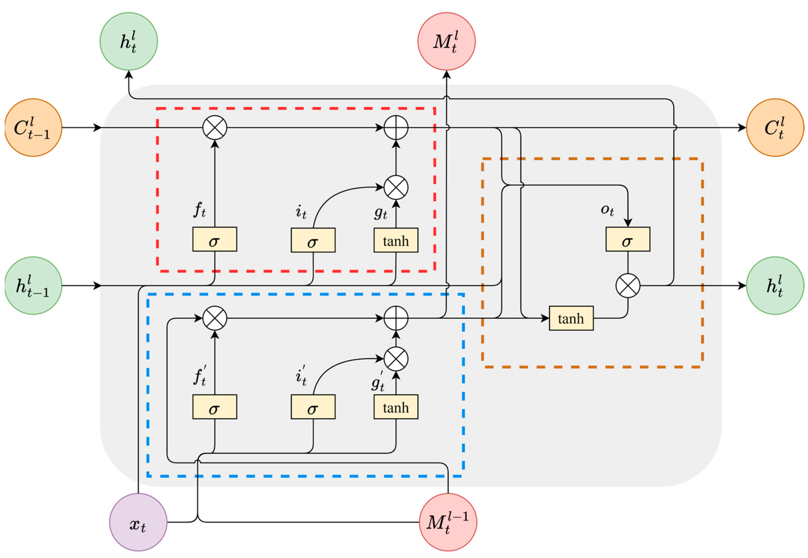
3.1. ST-LSTM

ST-LSTM is a variant of LSTM that adds spatial memory states. An ST-LSTM unit can be decomposed into three parts: the temporal memory state calculation part, the spatial memory state calculation part, and the hidden layer state calculation part. Figure 1 shows the internal structure of an ST-LSTM unit.

The temporal memory state (represented by ${\mathit{C}}_{\mathit{t}}^{\mathit{l}}$) calculation part is shown in the red box in Figure 1. In fact, it retains the structure of the input gate and the forget gate in LSTM, updating and transmitting in the time dimension. The computation of this part is shown as follows:

$$g_t=tanh(W_{xg}\ast x_t+W_{hg}\ast h_{t-1}^l+b_g),$$

(2)

$$i_t=\sigma \left(W_{xi}\ast x_t+W_{hi}\ast h_{t-1}^l+b_i\right),$$

(3)

$$f_t=\sigma \left(W_{xf}\ast x_t+W_{hf}\ast h_{t-1}^l+b_f\right),$$

(4)

$$C_t^l=f_t\odot C_{t-1}^l+i_t\odot g_t,$$

(5)

where $x_t$ is the input at time t, $C_t^l$ is the temporal memory state of layer $l$ at time $t$, and $h_{t-1}^l$ is the hidden state of the ST-LSTM unit of layer $l$ at time $t-1$. $g_t$, $i_t$, and $f_t$ are the input modulation gate, input gate, and forget gate of this part. * represents the convolution operation, and ⊙ is the Hadamard product.

In multichannel feature sequences, there are some features that are important for TEC prediction and need to be memorized and passed down. And there are also some that are not important and need to be discarded and forgotten. The forget gate $f_t$ is used to control the features that need to be discarded in the historical sequence. The input gate $i_{t }$ represents the multichannel features input at the current time. The memory state $C_t^l$ indicates how much of the past features are important to be remembered and passed down.

The spatial memory state (represented by ${\mathit{M}}_{\mathit{t}}^{\mathit{l}}$) calculation part is shown in the blue box in Figure 1. It also draws on the structure of the input gate and forget gate of LSTM. Unlike the temporal memory state that updates horizontally along the time direction, the spatial memory state updates and transfers vertically between layers. The calculations of this part are shown as follows:

$$g_t^{\prime }=tanh(W_{xg}^{\prime }\ast x_t+W_{mg}\ast M_t^{l-1}+b_g^{\prime }),$$

(6)

$$i_t^{\prime }=\sigma \left(W_{xi}^{\prime }\ast x_t+W_{mi}\ast M_t^{l-1}+b_i^{\prime }\right),$$

(7)

$$f_t^{\prime }=\sigma \left(W_{xf}^{\prime }\ast x_t+W_{mf}\ast M_t^{l-1}+b_f^{\prime }\right),$$

(8)

$$M_t^l=f_t^{\prime }\odot M_t^{l-1}+i_t^{\prime }\odot g_t^{\prime },$$

(9)

The hidden layer state (represented by ${\mathit{h}}_{\mathit{t}}^{\mathit{l}}$) calculation part is shown in the brown box in Figure 1. It is similar to the output gate in LSTM, responsible for integrating temporal and spatial memory and passing them on. The calculations of this part are shown as follows:

$$o_t=\sigma (W_{xo}\ast x_t+W_{ho}\ast h_{t-1}^l+W_{co}\ast C_t^l+W_{mo}\ast M_t^l+b_o),$$

(10)

$$h_t^l=o_t\odot \mathit{tanh}\left(W_{1\times 1}\ast \left[C_t^l,M_t^l\right]\right),$$

(11)

where $W_{1\times 1}$ represents a 1 × 1 weight matrix used for dimension reduction, and [] is a tensor concatenation.

3.2. PredRNN

PredRNN is a deep learning model structured by ST-LSTM units in a zigzag way. The zigzag connection is one of the innovations of the PredRNN network. Figure 2 shows the structures of PredRNN. Clearly, as shown in Figure 2, in PredRNN, in addition to temporal memory (C) being transmitted horizontally, there is also spatial memory (M) being transmitted in a zigzag pattern, which allows the spatial memory of the top-level from the previous time step to be transferred to the bottom layer at the next time step. In the previous time step, the spatial memory state is transmitted from bottom to top, recording changes in the spatial features of the data. Then, the spatial memory state from the top of the previous time step is transmitted to the bottom of the next time step and used for prediction. This dual-memory flow pattern helps PredRNN generate more accurate prediction results [36,44]. From Figure 2, it can also be seen that the PredRNN network adopts a standard n vs. n structure. It is also called a sequence–sequence structure. In this structure, the input data, the processed features of each layer, and the final output are all sequences of the same length. The structure of n vs. n limits the application of PredRNN.

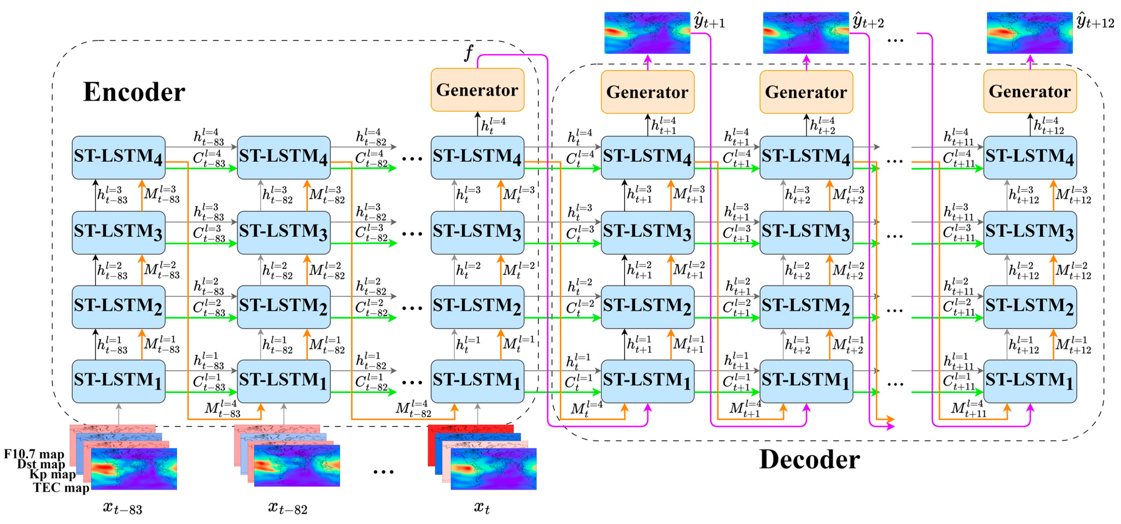
3.3. Encoder–Decoder Structure

The encoder–decoder structure is a fundamental approach in deep learning model design, which takes a sequence as input, converts the sequence into a feature vector, and then converts the feature vector into an output sequence. This sequence–vector–sequence structure is generally considered more effective than the sequence–sequence structure [45].

The deep learning model with encoder–decoder structure usually consists of two parts: the encoder part and the decoder part. The encoder part receives complex raw high-dimensional data and converts them into a low-dimensional feature vector, similar to feature extraction in traditional machine learning. The decoder part receives feature vectors and converts them back into high-dimensional outputs, which can typically be considered to be data recovery and reconstruction.

3.4. The Proposed Multichannel ED-PredRNN

This paper modifies the n vs. n structure in the original PredRNN to an encoder–decoder structure to address the issue of unequal input and output lengths in TEC prediction. Meanwhile, to improve the prediction performance, our proposed model allows multichannel features as input. The proposed Multichannel ED-PredRNN includes two parts, an encoder and a decoder, as shown in Figure 3.

The encoder receives multichannel data from the past 7 days (The length of the input is determined experimentally. We tried different input lengths and found that the prediction performance was best when the input length was 7 days.), calculates the spatial memory state $M_t^{l=4}$ and temporal memory state $C_t^l$, as well as the spatiotemporal feature vector $f$. This part consists of 4 layers of ST-LSTM units, which are used to extract the spatiotemporal features from multichannel data at each moment. These spatiotemporal features are not directly converted into predictions, but are merged into the final spatiotemporal feature vector (represented by $f$) through a generator unit composed of a two-dimensional convolutional layer (Conv2D) with a kernel size of 3 × 3 and sigmoid activation function. This spatiotemporal feature vector is then passed to the decoder part and converted into predictions.

The decoder receives temporal memory state, spatial memory state, and spatiotemporal feature vector, and uses a step-by-step prediction approach to predict the 12 TEC maps for the next day. This part also consists of 4 layers of ST-LSTM units and a generator, where the generator is the same as the one in the encoder part.

4. Experiments Setting

All models in this paper were built using Pytorch. The iteration number during training is set to 300, and the optimizer is set to Adaptive Motion Estimation (ADAM). The learning rate adopts a dynamic adjustment strategy, with an initial value of 0.003 and a decay rate of half every 50 times. The loss function of the model adopts the Structural Similarity Index Measure (SSIM). Research has shown that SSIM performs better in image prediction [46].

4.1. Evaluation Metrics

The evaluation metrics used in this paper are Root Mean Square Error (RMSE), Mean Absolute Percentage Error (MAPE), and coefficient of determination (${\mathrm{R}}^2$), which are calculated as follows:

$$RMSE=\sqrt{{\displaystyle \frac{1}{m}}{\sum }_{i=1}^m{(y_i-{\widehat{y}}_i)}^2},$$

(12)

$$MAPE={\displaystyle \frac{1}{m}}\sum _{i=1}^m\left|{\displaystyle \frac{y_i-{\widehat{y}}_i}{y_i}}\right|\times 100\%,$$

(13)

$$R^2=1-{\displaystyle \frac{\sum _{i=1}^m{\left({\widehat{y}}_i-y_i\right)}^2}{\sum _{i=1}^m{\left(y_i-\overline{y}\right)}^2}},$$

(14)

where $m\mathrm{ }$ is the total number of test samples, ${\widehat{y}}_i$ and $y_i$ represent the predicted value and ground truth of sample $i$, respectively, and $\overline{y}$ denotes the mean of all the ground truths.

4.2. Structure of Comparative Models

To verify the performance of the proposed model, this paper compared it with 3 state-of-the-art ionospheric TEC prediction models, including ConvLSTM, ConvGRU, and COPG. Among them, ConvLSTM and ConvGRU are mainstream deep learning models in TEC prediction, and COPG is a daily prediction product provided by CODE, which can be regarded as a benchmark. COPG can be downloaded from https://cddis.nasa.gov/archive/gnss/products/ionex/ (accessed on 3 April 2025). For a fair comparison, both ConvLSTM and ConvGRU adopt a similar encoder–decoder structure as the proposed Multichannel ED-PredRNN, as shown in Figure 4.

4.3. Model Optimization

In the proposed Multichannel ED-PredRNN, as well as the comparison models ConvLSTM and ConvGRU, there are hyper-parameters that have significant impacts on their performances. This paper uses the Bayesian optimization method to optimize the two most important hyper-parameters, the number of convolution kernels (represented by filter) and the size of convolution kernels (represented by kernel size). The optimal hyper-parameter combinations found by the Bayesian optimization algorithm for each model are shown in

Table 2. The best hyper-parameters found by Bayesian optimization.

Model	Hyper-Parameter Setting
	Filter	Kernel Size
Multichannel ED-PredRNN	9	9
ConvLSTM	16	3
ConvGRU	12	3

. In the subsequent experiments, the number and size of convolution kernels in each model were set to the values in Table 2.

5. Result and Discussion

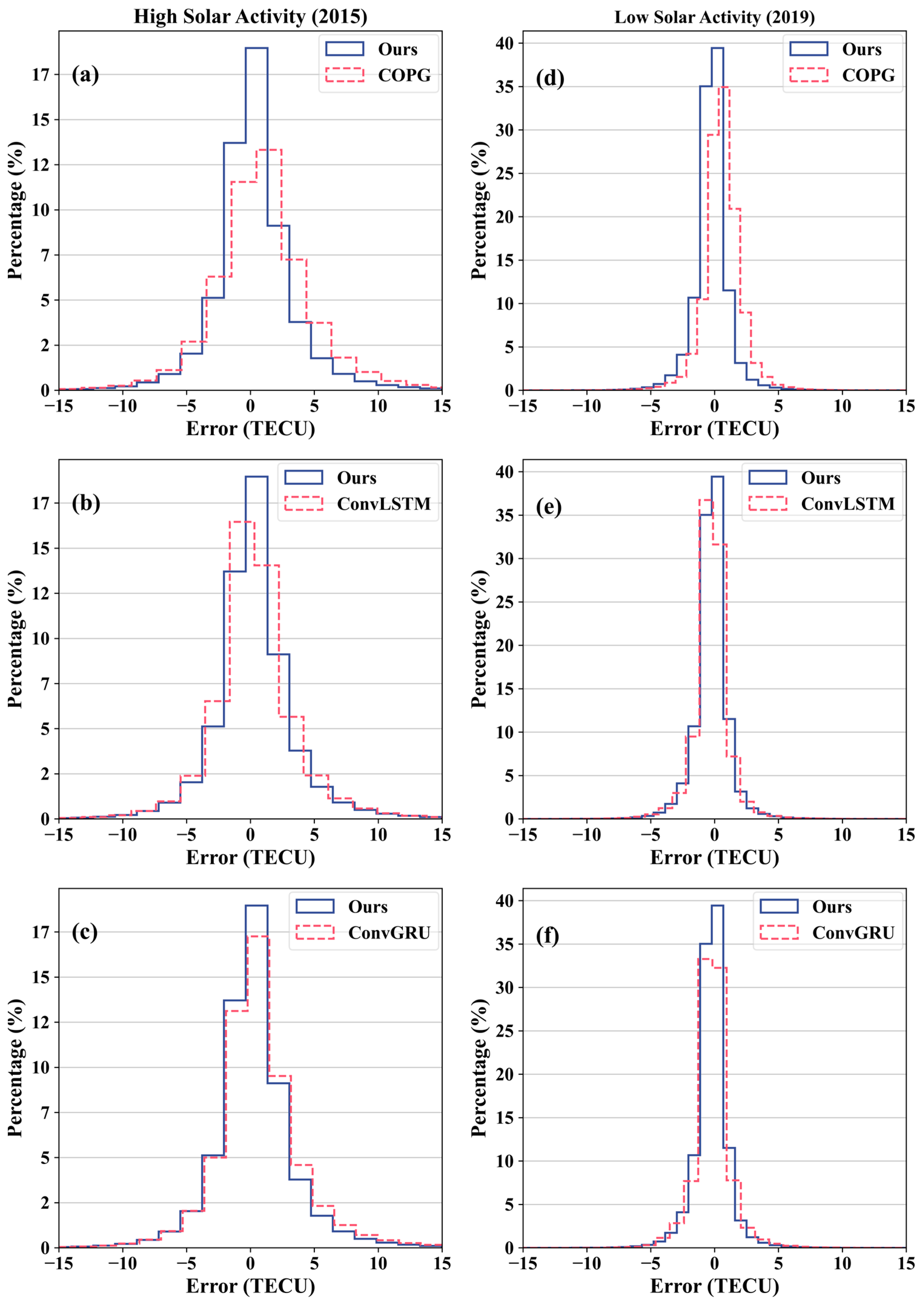
5.1. Overall Comparison Under Different Solar Activities

Table 3. Overall comparison under different solar activities.

Year and Solar Activity	Model	RMSE (TECU)	R2	MAPE (%)
2015, high solar activity	COPG	4.227	0.9321	19.89
	ConvLSTM	3.563	0.9518	15.32
	ConvGRU	3.757	0.9464	15.59
	Multichannel ED-PredRNN	3.374	0.9567	14.22
2019, low solar activity	COPG	1.618	0.9268	19.32
	ConvLSTM	1.559	0.9320	17.29
	ConvGRU	1.561	0.9319	17.96
	Multichannel ED-PredRNN	1.483	0.9385	15.76

presents the quantitative comparison results of four models, including $RMSE$, $MAPE$, and ${\mathrm{R}}^2$. Compared with COPG, ConvLSTM, and ConvGRU, the $RMSE$ of our proposed model decreased by 20.18%, 5.30%, and 10.19% in 2015 (high solar activity), and by 8.34%, 4.87%, and 5.00% in 2019 (low solar activity), respectively. According to the $MAPE$, our model decreased by 28.51%, 7.18%, and 8.79% in 2015, and by 18.43%, 8.85%, and 12.25% in 2019. Obviously, whether in years of high solar activity or low solar activity, compared with the three comparative models, our proposed model has significant advantages in $\mathrm{R}\mathrm{M}\mathrm{S}\mathrm{E}$ and $\mathrm{M}\mathrm{A}\mathrm{P}\mathrm{E}$. In terms of ${\mathrm{R}}^2$, our model is also superior to the comparative models.

Furthermore, for a more detailed comparison, Figure 5 provides the paired comparisons of error (denoted by Δ, $\Delta ={\widehat{y}}_i-y_i$) distribution on the test set. In addition, we calculated the RMSE difference (denoted as ΔRMSE) between the Multichannel ED-PredRNN and the three comparison models at 71 × 73 grid points worldwide, using the Multichannel ED-PredRNN as a benchmark. The formula is as follows:

$${\Delta RMSE}_{i,j}^{comparative model}={\Delta RMSE}_{i,j}^{comparative model}-{RMSE}_{i,j}^{Multichannel ED-PredRNN},$$

(15)

where ${\Delta RMSE}_{i,j}^{comparativemodel}$ presents the difference in RMSE between a comparative model and Multichannel ED-PredRNN at point $(i,j)$. At the same time, we provided the percentage of ΔRMSE > 0, as shown in

Table 4. Statistics of ΔRMSE > 0.

Solar Activity	${\Delta \mathbf{R}\mathbf{M}\mathbf{S}\mathbf{E}}^{\mathit{c}\mathit{o}\mathit{m}\mathit{p}\mathit{a}\mathit{r}\mathit{a}\mathit{t}\mathit{i}\mathit{v}\mathit{e} \mathit{m}\mathit{o}\mathit{d}\mathit{e}\mathit{l}}$	$\mathbf{Proportion} \mathbf{of} \Delta \mathbf{R}\mathbf{M}\mathbf{S}\mathbf{E}>0$
High (2015)	${\Delta \mathrm{R}\mathrm{M}\mathrm{S}\mathrm{E}}^{\mathrm{C}\mathrm{O}\mathrm{P}\mathrm{G}}$	96.06%
	${\Delta \mathrm{R}\mathrm{M}\mathrm{S}\mathrm{E}}^{\mathrm{C}\mathrm{o}\mathrm{n}\mathrm{v}\mathrm{G}\mathrm{R}\mathrm{U}}$	98.71%
	${\Delta \mathrm{R}\mathrm{M}\mathrm{S}\mathrm{E}}^{\mathrm{C}\mathrm{o}\mathrm{n}\mathrm{v}\mathrm{L}\mathrm{S}\mathrm{T}\mathrm{M}}$	90.18%
Low (2019)	${\Delta \mathrm{R}\mathrm{M}\mathrm{S}\mathrm{E}}^{\mathrm{C}\mathrm{O}\mathrm{P}\mathrm{G}}$	92.07%
	${\Delta \mathrm{R}\mathrm{M}\mathrm{S}\mathrm{E}}^{\mathrm{C}\mathrm{o}\mathrm{n}\mathrm{v}\mathrm{G}\mathrm{R}\mathrm{U}}$	80.28%
	${\Delta \mathrm{R}\mathrm{M}\mathrm{S}\mathrm{E}}^{\mathrm{C}\mathrm{o}\mathrm{n}\mathrm{v}\mathrm{L}\mathrm{S}\mathrm{T}\mathrm{M}}$	71.87%

. A positive RMSE indicates that the RMSE of the comparison model at $(i,j)$ is greater than that of Multichannel ED PredRNN, which means that at this point, the comparison model is inferior to Multichannel ED-PredRNN, and vice versa.

Obviously, compared to the other three models, the proposed Multichannel ED-PredRNN exhibits the highest proportion of errors near zero, both in years of high and low solar activities. This suggests that Multichannel ED-PredRNN surpasses the comparative models both in high and low solar activities.

To compare the four models more intuitively, this paper selects DOY102, 2015 (high solar activity year) and DOY26, 2019 (low solar activity year) to visually demonstrate the predictive effect of each model. Figure 6 and Figure 7 show the predictions of each model on the selected two days, while Figure 8 and Figure 9 show the absolute error of each model at each grid point. Based on these four figures, our proposed Multichannel ED-PredRNN has the smallest absolute error high-value region compared with the three comparative models, which means that Multichannel ED-PredRNN’s predicted maps are closest to the true TEC maps, indicating Multichannel ED-PredRNN has the best predictive performance among the four models.

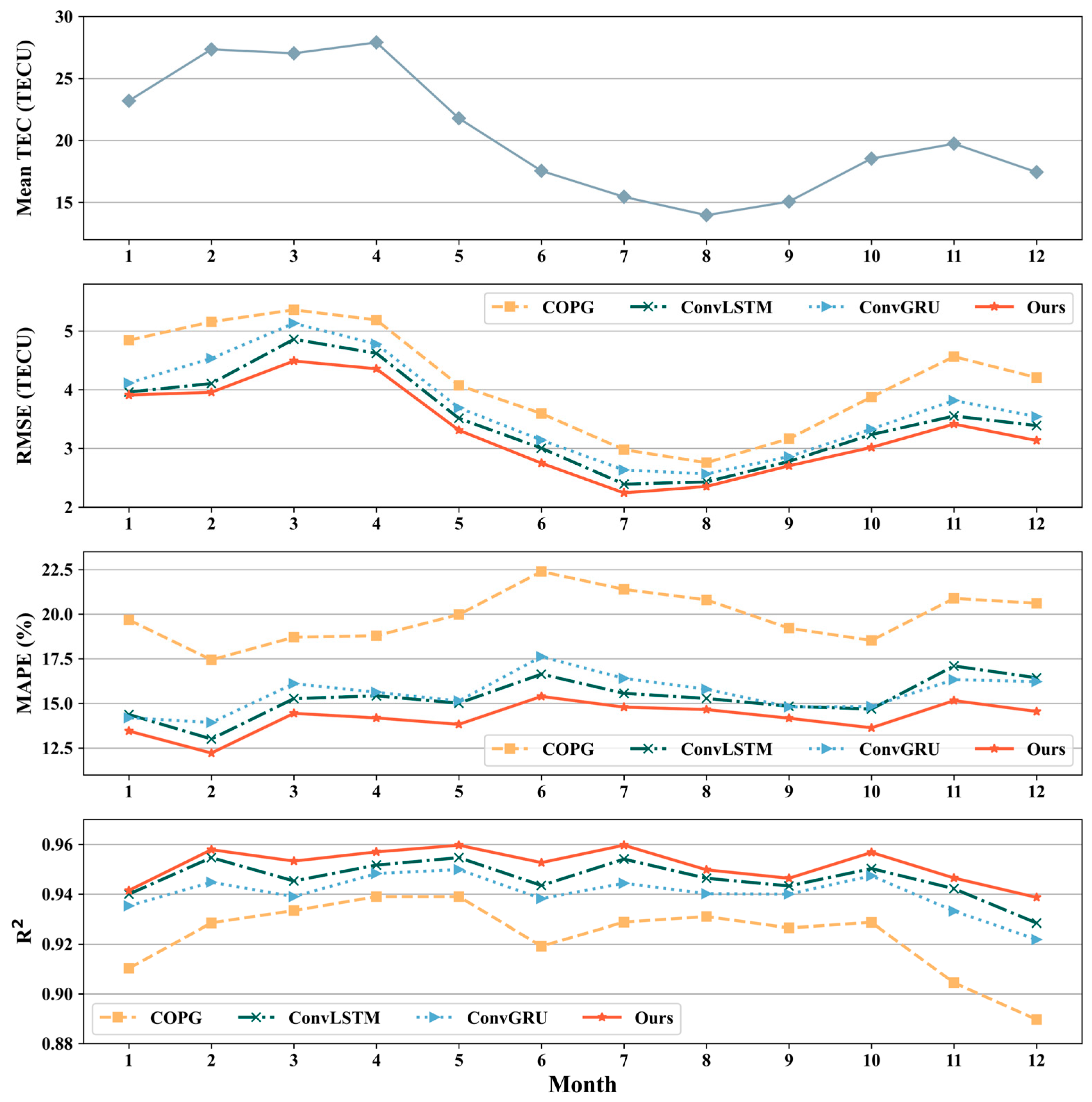
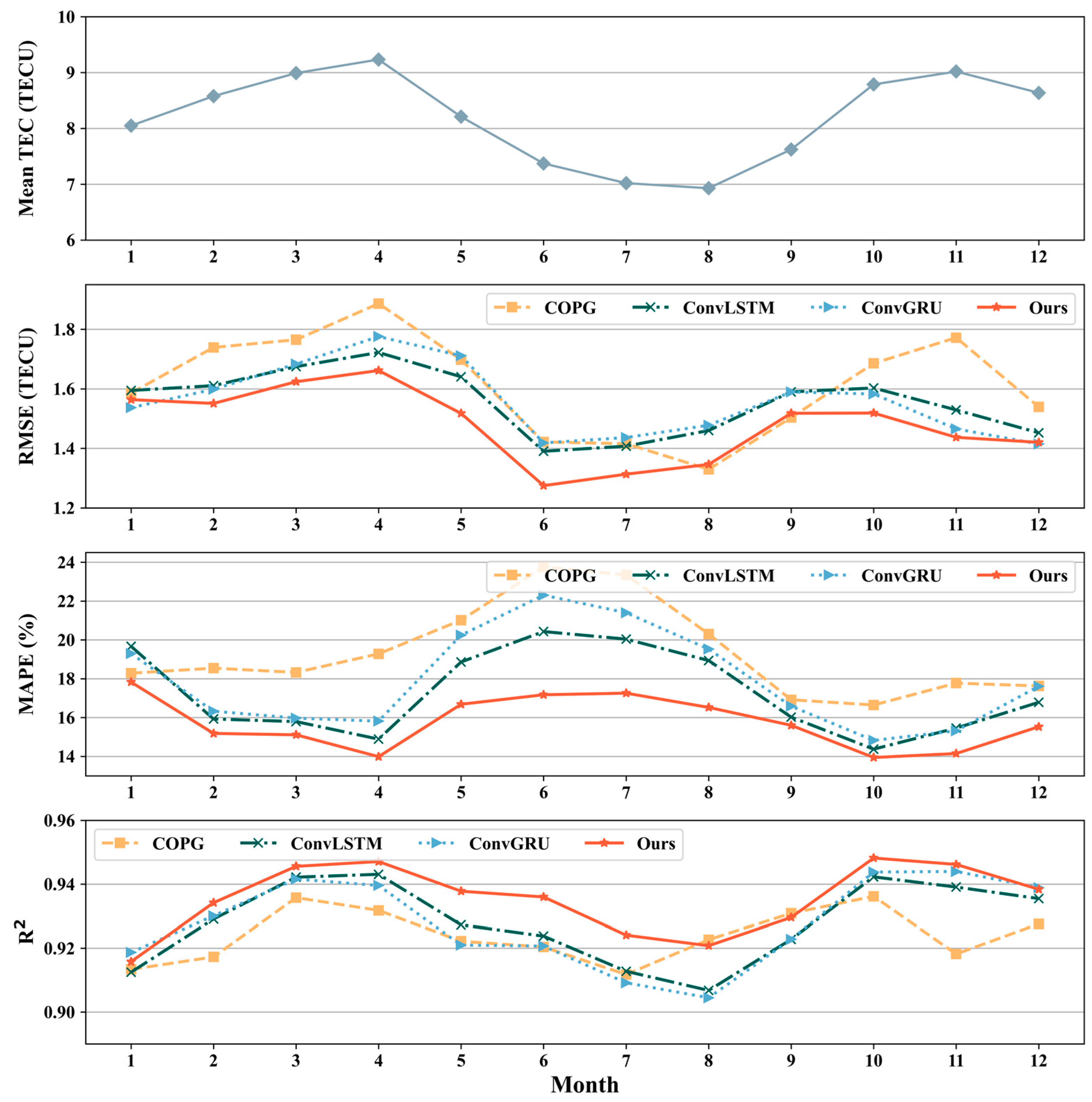
5.2. Comparison at Different Times

This section provides a monthly comparison of four models to compare the predictive performance of various models at different times, as shown in Figure 10 and Figure 11. Among them, the top row is the monthly mean values of the global TEC, and the other three rows are the monthly $\mathrm{R}\mathrm{M}\mathrm{S}\mathrm{E}$, $\mathrm{M}\mathrm{A}\mathrm{P}\mathrm{E}$, and ${\mathrm{R}}^2$, respectively.

In 2015, the monthly mean value of TEC first increased, reached its first peak in April, then decreased, and reached its lowest value in August. Then, it rose again, reaching its second peak in November, and then fell again. The $\mathrm{R}\mathrm{M}\mathrm{S}\mathrm{E}$ of each model has the same trend as that of the TEC mean; that is, when the monthly mean of TEC is large, the $\mathrm{R}\mathrm{M}\mathrm{S}\mathrm{E}$ of each model is also large, and vice versa. It means that the $\mathrm{R}\mathrm{M}\mathrm{S}\mathrm{E}$ of each model is linearly positively correlated with the monthly mean of TEC. The Pearson correlation coefficient is shown in

Table 5. Pearson correlation coefficient between RMSE and monthly average TEC of each model.

Pearson Correlation Coefficient	COPG	ConvLSTM	ConvGRU	Multichannel ED-PredRNN
2015	0.9397	0.9517	0.9651	0.9555
2019	0.9284	0.6921	0.5285	0.7363

.

In all 12 months of 2015, our Multichannel ED-PredRNN has the lowest $RMSE$. Among them, the superiority of the proposed Multichannel ED-PredRNN is most obvious in April when the monthly mean of TEC is the highest. At this point, the $RMSE$ of the Multichannel ED-PredRNN decreased by 16.02%, 5.69%, and 7.97% compared to COPG, ConvLSTM, and ConvGRU. From the perspective of $\mathrm{M}\mathrm{A}\mathrm{P}\mathrm{E}$, COPG’s $\mathrm{M}\mathrm{A}\mathrm{P}\mathrm{E}\mathrm{s}$ fluctuate around 20%, which is the worst. The $\mathrm{M}\mathrm{A}\mathrm{P}\mathrm{E}\mathrm{s}$ of Multichannel ED-PredRNN are below 15% in the vast majority of months and significantly lower than those of the three comparison models throughout the year. In addition, Multichannel ED-PredRNN has the highest ${\mathrm{R}}^2$ in every month of the year, also indicating its effectiveness compared to the three competitive models.

According to the monthly comparison in 2019 (low solar activity years), as shown in Figure 11, the $\mathrm{R}\mathrm{M}\mathrm{S}\mathrm{E}$ of each model is linearly positively correlated with the monthly mean of TEC, too. Our proposed Multichannel ED-PredRNN was slightly inferior to COPG in August and September, and slightly inferior to ConvGRU in January and December, ranking second. In the remaining 8 months, Multichannel ED-PredRNN is the best.

In summary, the monthly comparison indicates that Multichannel ED-PredRNN outperforms the 3 comparative models in the vast majority of months, whether in high or low solar activity years.

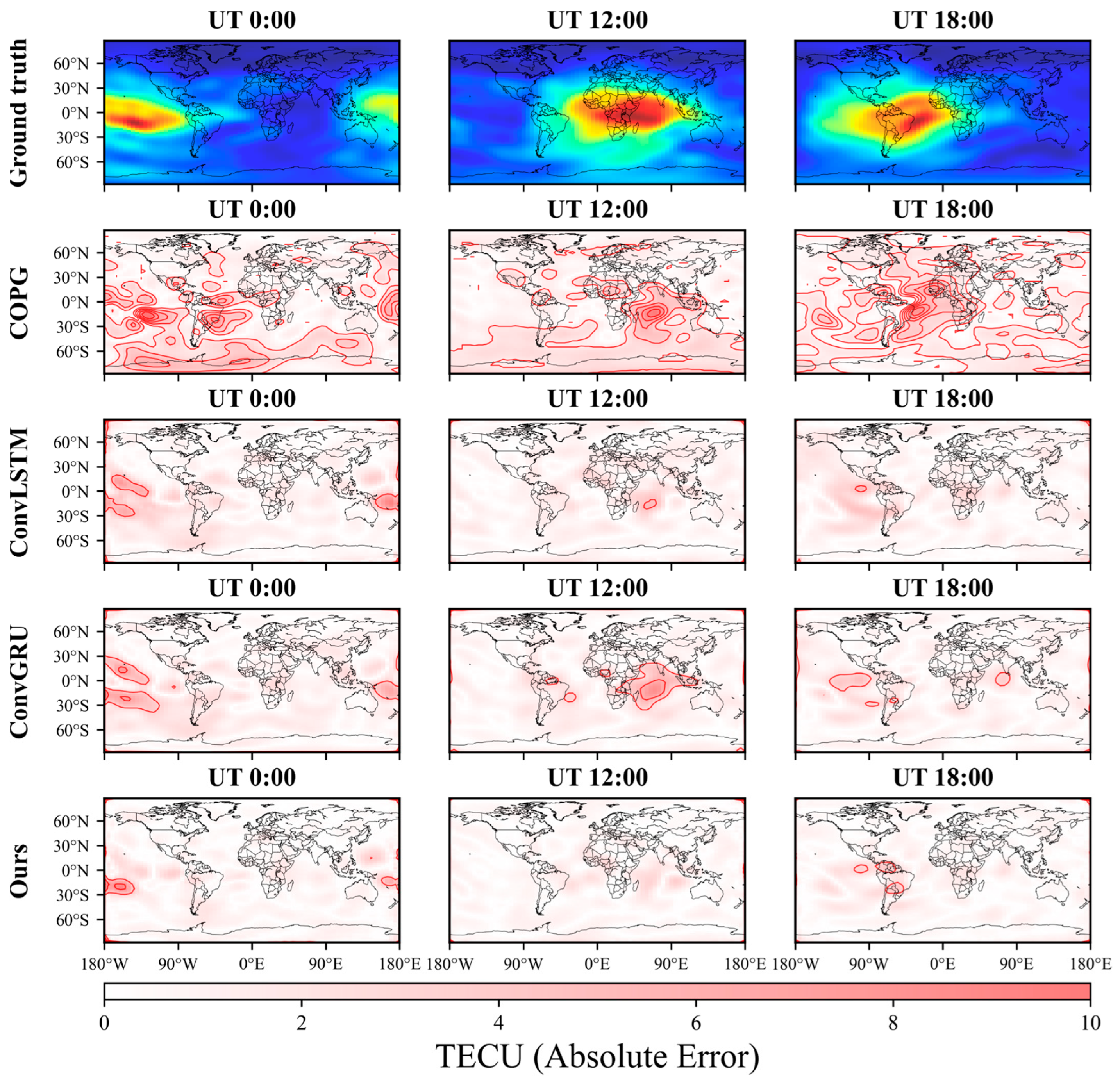
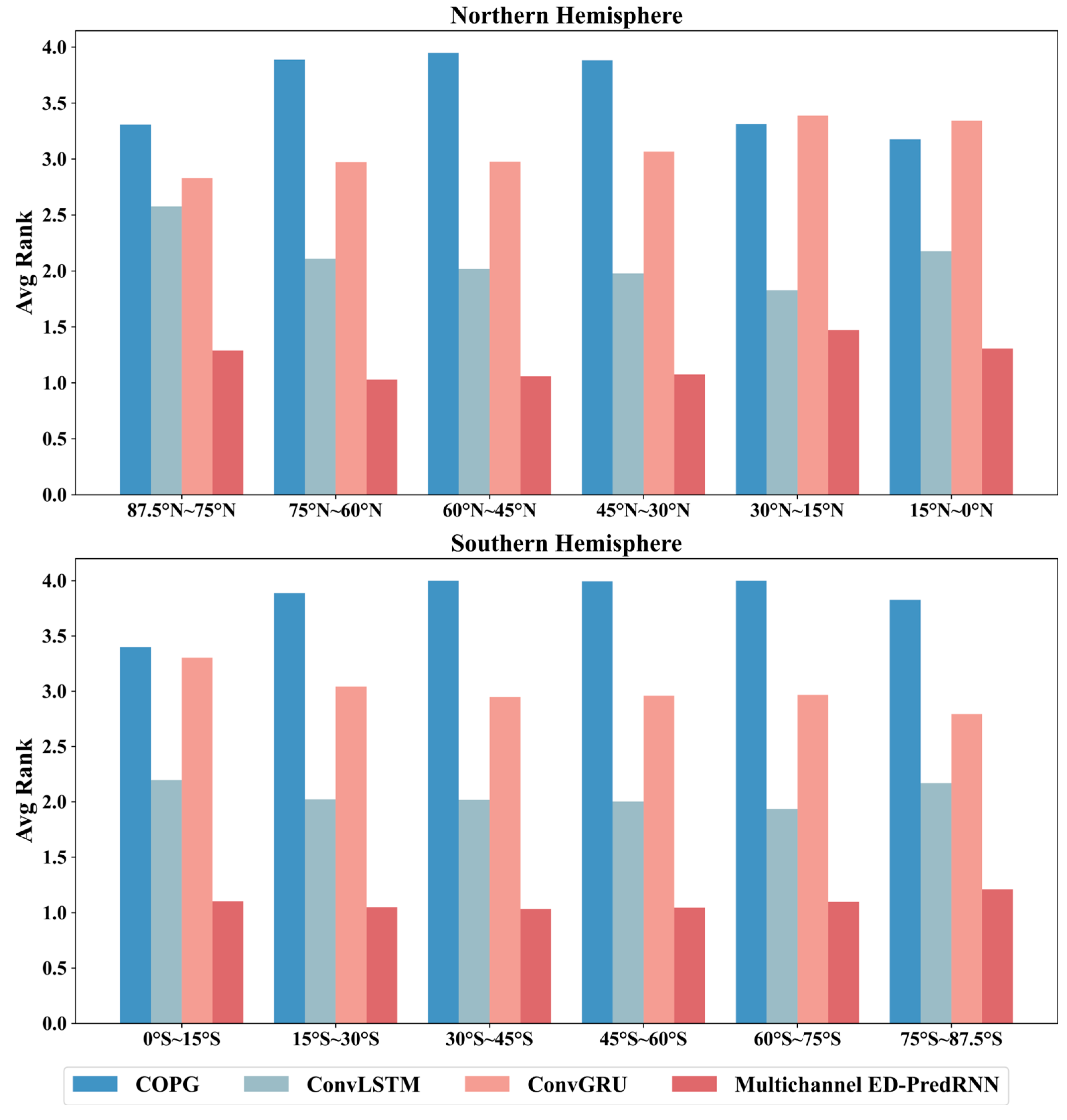
5.3. Comparison at Different Spatial Locations

This section divides the world into 12 subregions by latitude to compare the predictive performance of various models within different latitude regions. In each latitude region, the Friedman test method was carried out to rank the RMSEs of all the models. The average ranking of each model within each latitude region is shown in Figure 12, where a lower ranking indicates a better performance. It can be seen that Multichannel ED-PredRNN has the lowest average ranking in all 12 regions, indicating that Multichannel ED-PredRNN has the best average performance in all subregions.

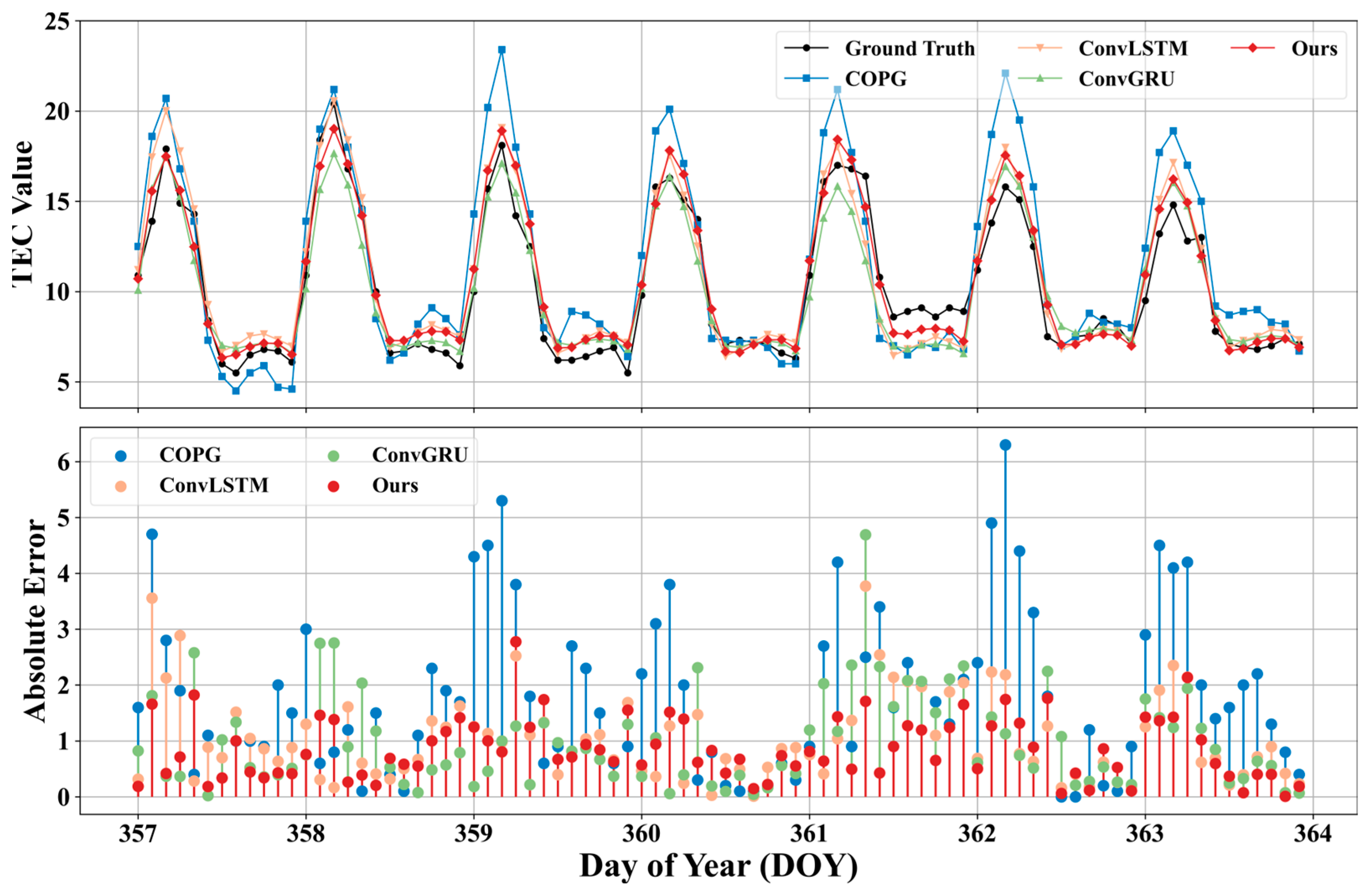
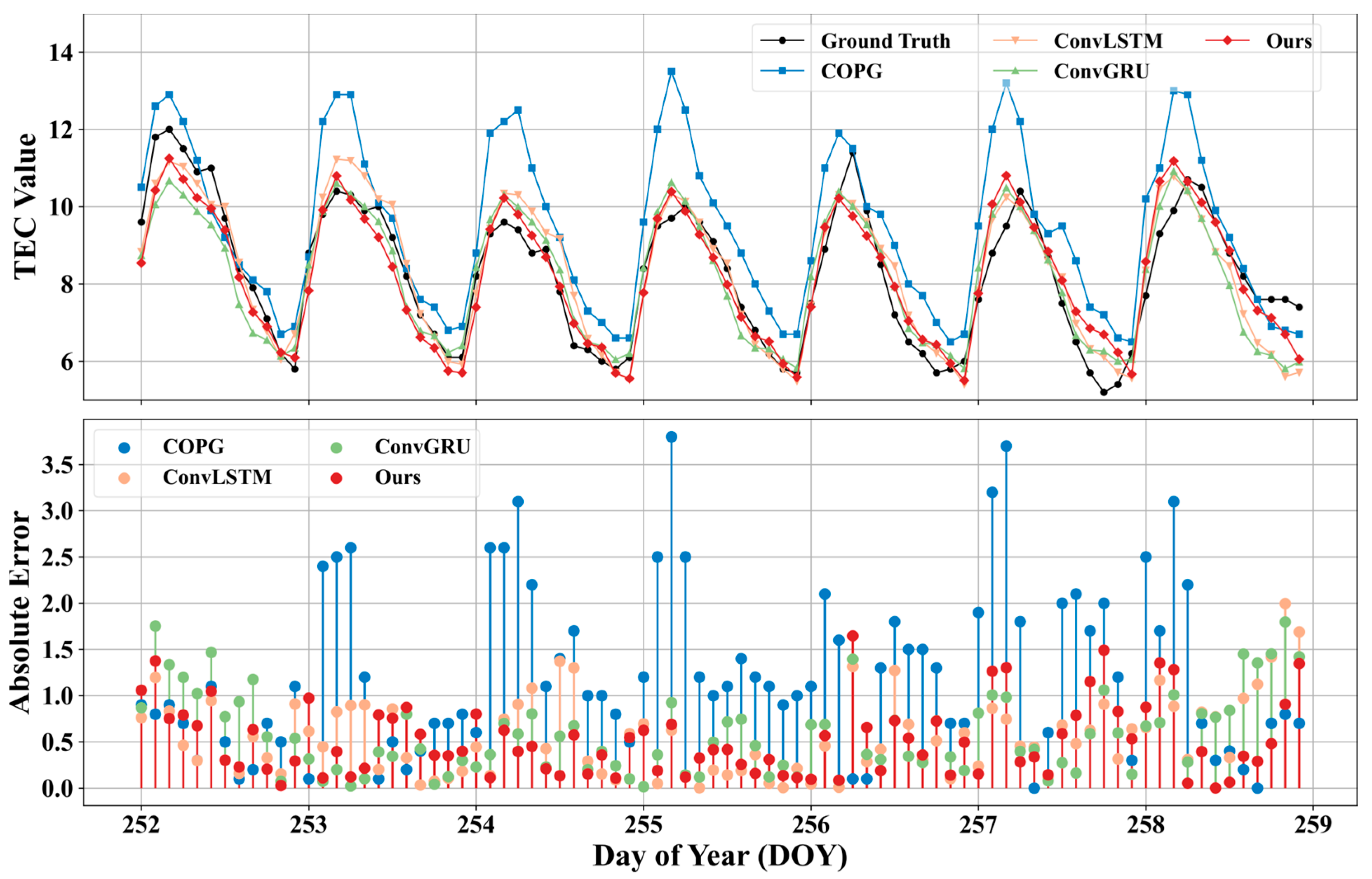
5.4. Single Site Prediction Analysis

This section takes the Beijing station (40° N, 115° E) as an example for single site prediction analysis.

Figure 13 and Figure 14 show single site prediction for 7 consecutive days in high solar activity years (DOY357-363, 2015) and low solar activity years (DOY252-DOY258, 2019), respectively. Among them, the top presents the predicted values of each model for 7 consecutive days, and the bottom shows their $\mathrm{R}\mathrm{M}\mathrm{S}\mathrm{E}\mathrm{s}$. According to Figure 13 and Figure 14, the $\mathrm{R}\mathrm{M}\mathrm{S}\mathrm{E}$ of each model is positively correlated with the ground truth. Overall, the $\mathrm{R}\mathrm{M}\mathrm{S}\mathrm{E}\mathrm{s}$ of Multichannel ED-PredRNN are the lowest in the vast majority of cases, indicating that on Beijing station, Multichannel ED-PredRNN is superior to the comparative models.

5.5. Comparison Under Extreme Situations

This section validates the effectiveness of the Multichannel ED-PredRNN in extreme situations. To achieve this goal, we selected a geomagnetic storm event that occurred on DOY354, 2015. In this geomagnetic storm event, the minimum Dst was -166 nT. According to the classification criteria of geomagnetic storm levels [26], it belongs to a major geomagnetic storm. To cover the entire process of the geomagnetic storm as much as possible, we took the minimum Dst day as the center, and took 4 days before and after, namely DOY350-358, and compared Multichannel ED-PredRNN with COPG, ConvLSTM, and ConvGRU during this period.

Figure 15 shows the performance of four models during this geomagnetic storm period. Figure 15a shows the Dst index, which is used to reflect the intensity of magnetic storms. Figure 15b,c present the $\mathrm{R}\mathrm{M}\mathrm{S}\mathrm{E}$ and ${\mathrm{R}}^2$, respectively. From the Dst curve in Figure 15a, it can be seen that during DOY354-355, 2015, Dst is less than −100 nT, indicating a major storm had occurred. During these two days, the $\mathrm{R}\mathrm{M}\mathrm{S}\mathrm{E}$ of each model significantly increased and ${\mathrm{R}}^2$ decreased, indicating that the performances of all models declined during the geomagnetic storm period. Nevertheless, the proposed Multichannel ED-PredRNN demonstrated better performance than other models. In addition, we also found that the performance of each model deteriorates when there is a disturbance in the Dst curve, especially when a local minimum Dst appears. We labeled 10 local minimum points on the Dst curve with rectangular boxes (1)–(10). It can be seen that there is a good one-to-one correspondence between the local maximum points of $\mathrm{R}\mathrm{M}\mathrm{S}\mathrm{E}$ and the local minimum points of Dst. As for ${\mathrm{R}}^2$, there is also a similar correspondence relationship. Among them, on 6 out of 10 points (marked in blue), the $\mathrm{R}\mathrm{M}\mathrm{S}\mathrm{E}$ local maximum and the Dst local minimum appear simultaneously. At 6 points (marked in green), the local maximum of $\mathrm{R}\mathrm{M}\mathrm{S}\mathrm{E}$ lags behind the corresponding local minimum of Dst by 2 h. At 1 point (marked in yellow), the local maximum of $\mathrm{R}\mathrm{M}\mathrm{S}\mathrm{E}$ is 2 h ahead of the local minimum of Dst. These indicate that the predictive performance of each model deteriorates when local minima occur in Dst. From Figure 15, it can be seen that COPG is most severely affected by Dst, while our Multichannel ED-PredRNN is least affected by Dst. This once again demonstrates that the Multichannel ED-PredRNN, which adopts the dual memory mechanism and zigzag connection pattern can effectively utilize the temporal and spatial features in the sequence, thereby improving the accuracy of TEC prediction.

6. Conclusions

To improve the performance of TEC prediction, it is necessary to fully utilize the spatial and temporal features in historical data as much as possible. Therefore, this paper chose ST-LSTM with both temporal and spatial memory mechanisms as the basic feature extraction unit and proposed a Multichannel ED-PredRNN. In our model, an encoder–decoder structure is used to lay out ST-LSTM units. In the encoder, a generator is applied to integrate the output sequence from ST-LSTM units into a spatiotemporal feature vector. In the decoder, the spatiotemporal feature vector is decoded by the ST-LSTM units and converted into an output TEC sequence by the generator. This design approach allows the PredRNN to handle situations where the input length and output length are not equal. In addition, we aligned Dst, F10.7, and Kp into map data that are consistent with the temporal and spatial resolution of global TEC maps, and overlaid these maps with TEC maps to form multichannel features. Then, we input these multichannel features together into the Multichannel ED-PredRNN to improve its accuracy. The Multichannel ED-PredRNN is compared with three mainstream models, COPG, ConvLSTM, and ConvGRU, from multiple perspectives. Comparative experiments include (1) overall comparison under different solar activities; (2) comparison at different times; (3) comparison at different spatial locations; (4) single site prediction analysis; and (5) comparison under extreme situations. The main conclusions drawn are as follows:

• The overall comparison between high and low solar activity years shows that Multichannel ED-PredRNN outperforms COPG, ConvLSTM, and ConvGRU. Comparing these three models, the $\mathrm{R}\mathrm{M}\mathrm{S}\mathrm{E}$ of Multichannel ED-PredRNN decreased by 20.18%, 5.30%, and 10.19% in 2015 (high solar activity), and by 8.34%, 4.87%, and 5.00% in 2019 (low solar activity).
• Comparison at different times indicates that the $\mathrm{R}\mathrm{M}\mathrm{S}\mathrm{E}$ of each model is linearly positively correlated with the monthly mean of TEC. In all 12 months of 2015 and 8 months of 2019, Multichannel ED-PredRNN performs the best.
• Comparison at different spatial locations shows that Multichannel ED-PredRNN ranks first in all 12 subregions globally.
• The single station prediction using Beijing Station as an example shows that in the vast majority of cases, Multichannel ED-PredRNN outperforms the comparative models, especially at the peaks of TEC.
• The comparison in extreme cases (such as geomagnetic storms) shows that the predictive performance of all models is affected by geomagnetic disturbances, while Multichannel ED-PredRNN is least affected by geomagnetic disturbances.

There is still room for improvement in this study. In this article, only Kp, Dst, and F10.7 were used as auxiliary features for TEC prediction. However, other factors such as tidal effects or AGWs are also related to TEC. In the future, more factors will be considered in TEC modeling.

References

- Monte-Moreno, E.; Yang, H.; Hernández-Pajares, M. Forecast of the Global TEC by Nearest Neighbour Technique. Remote Sens. 2022, 14, 1361. [Google Scholar] [CrossRef]
- Xiong, B.; Li, X.; Wang, Y.; Zhang, H.; Liu, Z.; Ding, F.; Zhao, B. Prediction of ionospheric TEC over China based on long and short-term memory neural network. Chin. J. Geophys. 2022, 65, 2365–2377. [Google Scholar] [CrossRef]
- Ray, S.; Huba, J.D.; Kundu, B.; Jin, S. Influence of the October 14, 2023, Ring of Fire Annular Eclipse on the Ionosphere: A Comparison Between GNSS Observations and SAMI3 Model Prediction. JGR Space Phys. 2024, 129, e2024JA032710. [Google Scholar] [CrossRef]
- Sun, Y.-Y.; Shen, M.M.; Tsai, Y.-L.; Lin, C.-Y.; Chou, M.-Y.; Yu, T.; Lin, K.; Huang, Q.; Wang, J.; Qiu, L.; et al. Wave Steepening in Ionospheric Total Electron Density Due to the 21 August 2017 Total Solar Eclipse. J. Geophys. Res. Space Phys. 2021, 126, e2020JA028931. [Google Scholar] [CrossRef]
- Bilitza, D.; Altadill, D.; Truhlik, V.; Shubin, V.; Galkin, I.; Reinisch, B.; Huang, X. International Reference Ionosphere 2016: From Ionospheric Climate to Real-time Weather Predictions. Space Weather 2017, 15, 418–429. [Google Scholar] [CrossRef]
- Hochegger, G.; Nava, B.; Radicella, S.; Leitinger, R. A Family of Ionospheric Models for Different Uses. Phys. Chem. Earth Part C Sol. Terr. Planet. Sci. 2000, 25, 307–310. [Google Scholar] [CrossRef]
- Nava, B.; Coïsson, P.; Radicella, S.M. A New Version of the NeQuick Ionosphere Electron Density Model. J. Atmos. Sol.-Terr. Phys. 2008, 70, 1856–1862. [Google Scholar] [CrossRef]
- Bent, R.B.; Llewellyn, S.K.; Nesterczuk, G.; Schmid, P.E. The Development of a Highly-Successful Worldwide Empirical Ionospheric Model and Its Use in Certain Aspects of Space Communications and Worldwide Total Electron Content Investigations; Naval Research Laboratory: Washington, DC, USA, 1975; pp. 13–28. [Google Scholar]
- Rawer, K.; Bilitza, D.; Ramakrishnan, S. Goals and Status of the International Reference Ionosphere. Rev. Geophys. 1978, 16, 177–181. [Google Scholar] [CrossRef]
- Lin, X.; Wang, H.; Zhang, Q.; Yao, C.; Chen, C.; Cheng, L.; Li, Z. A Spatiotemporal Network Model for Global Ionospheric TEC Forecasting. Remote Sens. 2022, 14, 1717. [Google Scholar] [CrossRef]
- Bilitza, D. International Reference Ionosphere: Recent Developments. Radio Sci. 1986, 21, 343–346. [Google Scholar] [CrossRef]
- Li, Z.-G.; Cheng, Z.-Y.; Feng, C.-G.; Li, W.-C.; Li, H.-R. A Study of Prediction Models for Ionosphere. Chin. J. Geophys. 2007, 50, 307–319. [Google Scholar]
- Ratnam, D.V.; Otsuka, Y.; Sivavaraprasad, G.; Dabbakuti, J.R.K.K. Development of Multivariate Ionospheric TEC Forecasting Algorithm Using Linear Time Series Model and ARMA over Low-Latitude GNSS Station. Adv. Space Res. 2019, 63, 2848–2856. [Google Scholar] [CrossRef]
- Mandrikova, O.V.; Fetisova, N.V.; Al-Kasasbeh, R.T.; Klionskiy, D.M.; Geppener, V.V.; Ilyash, M.Y. Ionospheric Parameter Modelling and Anomaly Discovery by Combining the Wavelet Transform with Autoregressive Models. Ann. Geophys. 2015, 58, 1. [Google Scholar] [CrossRef]
- Kaselimi, M.; Voulodimos, A.; Doulamis, N.; Doulamis, A.; Delikaraoglou, D. Deep Recurrent Neural Networks for Ionospheric Variations Estimation Using GNSS Measurements. IEEE Trans. Geosci. Remote Sens. 2022, 60, 5800715. [Google Scholar] [CrossRef]
- Akhoondzadeh, M. A MLP Neural Network as an Investigator of TEC Time Series to Detect Seismo-Ionospheric Anomalies. Adv. Space Res. 2013, 51, 2048–2057. [Google Scholar] [CrossRef]
- Hochreiter, S.; Schmidhuber, J. Long Short-Term Memory. Neural Comput. 1997, 9, 1735–1780. [Google Scholar] [CrossRef]
- Ruwali, A.; Kumar, A.J.S.; Prakash, K.B.; Sivavaraprasad, G.; Ratnam, D.V. Implementation of Hybrid Deep Learning Model (LSTM-CNN) for Ionospheric TEC Forecasting Using GPS Data. IEEE Geosci. Remote Sens. Lett. 2021, 18, 1004–1008. [Google Scholar] [CrossRef]
- Sun, W.; Xu, L.; Huang, X.; Zhang, W.; Yuan, T.; Chen, Z.; Yan, Y. Forecasting of Ionospheric Vertical Total Electron Content (TEC) Using LSTM Networks. In Proceedings of the 2017 International Conference on Machine Learning and Cybernetics (ICMLC), IEEE, Ningbo, China, 9–12 July 2017; pp. 340–344. [Google Scholar]
- Tang, J.; Li, Y.; Yang, D.; Ding, M. An Approach for Predicting Global Ionospheric TEC Using Machine Learning. Remote Sens. 2022, 14, 1585. [Google Scholar] [CrossRef]
- Xiong, P.; Zhai, D.; Long, C.; Zhou, H.; Zhang, X.; Shen, X. Long Short-Term Memory Neural Network for Ionospheric Total Electron Content Forecasting Over China. Space Weather 2021, 19, e2020SW002706. [Google Scholar] [CrossRef]
- Tang, R.; Zeng, F.; Chen, Z.; Wang, J.-S.; Huang, C.-M.; Wu, Z. The Comparison of Predicting Storm-Time Ionospheric TEC by Three Methods: ARIMA, LSTM, and Seq2Seq. Atmosphere 2020, 11, 316. [Google Scholar] [CrossRef]
- Shi, X.; Chen, Z.; Wang, H.; Yeung, D.-Y.; Wong, W.; Woo, W. Convolutional LSTM Network: A Machine Learning Approach for Precipitation Nowcasting. 2015. Available online: https://proceedings.neurips.cc/paper/2015/hash/07563a3fe3bbe7e3ba84431ad9d055af-Abstract.html (accessed on 9 March 2025).
- Gao, X.; Yao, Y. A Storm-Time Ionospheric TEC Model with Multichannel Features by the Spatiotemporal ConvLSTM Network. J. Geod. 2023, 97, 9. [Google Scholar] [CrossRef]
- Liu, L.; Morton, Y.J.; Liu, Y. Machine Learning Prediction of Storm-Time High-Latitude Ionospheric Irregularities From GNSS-Derived ROTI Maps. Geophys. Res. Lett. 2021, 48, e2021GL095561. [Google Scholar] [CrossRef]
- Li, L.; Liu, H.; Le, H.; Yuan, J.; Shan, W.; Han, Y.; Yuan, G.; Cui, C.; Wang, J. Spatiotemporal Prediction of Ionospheric Total Electron Content Based on ED-ConvLSTM. Remote Sens. 2023, 15, 3064. [Google Scholar] [CrossRef]
- Hanson, A.; Pnvr, K.; Krishnagopal, S.; Davis, L. Bidirectional Convolutional LSTM for the Detection of Violence in Videos. In Computer Vision—ECCV 2018 Workshops; Leal-Taixé, L., Roth, S., Eds.; Lecture Notes in Computer Science; Springer International Publishing: Cham, Switzerland, 2019; Volume 11130, pp. 280–295. ISBN 978-3-030-11011-6. [Google Scholar]
- Chang, Y.; Luo, B. Bidirectional Convolutional LSTM Neural Network for Remote Sensing Image Super-Resolution. Remote Sens. 2019, 11, 2333. [Google Scholar] [CrossRef]
- Knol, D.; De Leeuw, F.; Meirink, J.F.; Krzhizhanovskaya, V.V. Deep Learning for Solar Irradiance Nowcasting: A Comparison of a Recurrent Neural Network and Two Traditional Methods. In Computational Science—ICCS 2021; Paszynski, M., Kranzlmüller, D., Krzhizhanovskaya, V.V., Dongarra, J.J., Sloot, P.M.A., Eds.; Lecture Notes in Computer Science; Springer International Publishing: Cham, Switzerland, 2021; Volume 12746, pp. 309–322. ISBN 978-3-030-77976-4. [Google Scholar]
- Yao, R.; Zhang, Y.; Gao, C.; Zhou, Y.; Zhao, J.; Liang, L. Lightweight Video Object Segmentation Based on ConvGRU. In Pattern Recognition and Computer Vision; Lin, Z., Wang, L., Yang, J., Shi, G., Tan, T., Zheng, N., Chen, X., Zhang, Y., Eds.; Lecture Notes in Computer Science; Springer International Publishing: Cham, Switzerland, 2019; Volume 11858, pp. 441–452. ISBN 978-3-030-31722-5. [Google Scholar]
- Tang, J.; Zhong, Z.; Hu, J.; Wu, X. Forecasting Regional Ionospheric TEC Maps over China Using BiConvGRU Deep Learning. Remote Sens. 2023, 15, 3405. [Google Scholar] [CrossRef]
- Chen, J.; Zhi, N.; Liao, H.; Lu, M.; Feng, S. Global Forecasting of Ionospheric Vertical Total Electron Contents via ConvLSTM with Spectrum Analysis. GPS Solut. 2022, 26, 69. [Google Scholar] [CrossRef]
- Sivakrishna, K.; Venkata Ratnam, D.; Sivavaraprasad, G. A Bidirectional Deep-Learning Algorithm to Forecast Regional Ionospheric TEC Maps. IEEE J. Sel. Top. Appl. Earth Obs. Remote Sens. 2022, 15, 4531–4543. [Google Scholar] [CrossRef]
- Xia, G.; Liu, M.; Zhang, F.; Zhou, C. CAiTST: Conv-Attentional Image Time Sequence Transformer for Ionospheric TEC Maps Forecast. Remote Sens. 2022, 14, 4223. [Google Scholar] [CrossRef]
- Zhukov, A.V.; Yasyukevich, Y.V.; Bykov, A.E. GIMLi: Global Ionospheric Total Electron Content Model Based on Machine Learning. GPS Solut. 2021, 25, 19. [Google Scholar] [CrossRef]
- Wang, Y.; Long, M.; Wang, J.; Gao, Z.; Yu, P.S. PredRNN: Recurrent Neural Networks for Predictive Learning Using Spatiotemporal LSTMs. In Proceedings of the Advances in Neural Information Processing Systems, Long Beach, CA, USA, 4–9 December 2017; Curran Associates, Inc.: Sydney, Australia, 2017; Volume 30. [Google Scholar]
- Li, W.; Zhu, H.; Shi, S.; Zhao, D.; Shen, Y.; He, C. Modeling China’s Sichuan-Yunnan’s Ionosphere Based on Multichannel WOA-CNN-LSTM Algorithm. IEEE Trans. Geosci. Remote Sens. 2024, 62, 5705018. [Google Scholar] [CrossRef]
- Xu, C.; Ding, M.; Tang, J. Prediction of GNSS-Based Regional Ionospheric TEC Using a Multichannel ConvLSTM With Attention Mechanism. IEEE Geosci. Remote Sens. Lett. 2024, 21, 1001405. [Google Scholar] [CrossRef]
- Feng, J.; Zhang, Y.; Li, W.; Han, B.; Zhao, Z.; Zhang, T.; Huang, R. Analysis of Ionospheric TEC Response to Solar and Geomagnetic Activities at Different Solar Activity Stages. Adv. Space Res. 2023, 71, 2225–2239. [Google Scholar] [CrossRef]
- Huang, L.; Wu, H.; Lou, Y.; Zhang, H.; Liu, L.; Huang, L. Spatiotemporal Analysis of Regional Ionospheric TEC Prediction Using Multi-Factor NeuralProphet Model under Disturbed Conditions. Remote Sens. 2022, 15, 195. [Google Scholar] [CrossRef]
- Ren, X.; Yang, P.; Mei, D.; Liu, H.; Xu, G.; Dong, Y. Global Ionospheric TEC Forecasting for Geomagnetic Storm Time Using a Deep Learning-Based Multi-Model Ensemble Method. Space Weather 2023, 21, e2022SW003231. [Google Scholar] [CrossRef]
- Tapping, K.F. The 10.7 Cm Solar Radio Flux (F10.7). Space Weather 2013, 11, 394–406. [Google Scholar] [CrossRef]
- Viereck, R.; Puga, L.; McMullin, D.; Judge, D.; Weber, M.; Tobiska, W.K. The Mg II Index: A Proxy for Solar EUV. Geophys. Res. Lett. 2001, 28, 1343–1346. [Google Scholar] [CrossRef]
- Wang, Y.; Wu, H.; Zhang, J.; Gao, Z.; Wang, J.; Yu, P.S.; Long, M. PredRNN: A Recurrent Neural Network for Spatiotemporal Predictive Learning. IEEE Trans. Pattern Anal. Mach. Intell. 2023, 45, 2208–2225. [Google Scholar] [CrossRef]
- Chen, G.; Hu, L.; Zhang, Q.; Ren, Z.; Gao, X.; Cheng, J. ST-LSTM: Spatio-Temporal Graph Based Long Short-Term Memory Network For Vehicle Trajectory Prediction. In Proceedings of the 2020 IEEE International Conference on Image Processing (ICIP), IEEE, Abu Dhabi, United Arab Emirates, 25–28 October 2020; pp. 608–612. [Google Scholar]
- Wang, Z.; Bovik, A.C.; Sheikh, H.R.; Simoncelli, E.P. Image Quality Assessment: From Error Visibility to Structural Similarity. IEEE Trans. Image Process. 2004, 13, 600–612. [Google Scholar] [CrossRef]
- Noll, C.E. The Crustal Dynamics Data Information System: A Resource to Support Scientific Analysis Using Space Geodesy. Adv. Space Res. 2010, 45, 1421–1440. [Google Scholar] [CrossRef]