Deep Learning for Atmospheric Modeling: A Proof of Concept Using a Fourier Neural Operator on WRF Data to Accelerate Transient Wind Forecasting at Multiple Altitudes

Abstract

This study addresses the problem of the computational cost of transient CFD simulations, which rely on iterative time-step calculations, by employing deep learning to generate optimized initial conditions for accelerating the Weather Research and Forecasting (WRF) model. To this end, we forecasted wind speed for short time frames over the Houston region using the WRF model data from 2019 to 2022, training the models to predict the X-component (U) wind speed. The so-called global FNO model, trained across all atmospheric heights, was first tested, achieving competitive results. A more refined approach was tested to improve it, training separate models for each altitude level, enhancing accuracy significantly. These ad hoc models outperformed surface and middle atmosphere persistence, achieving 27.64% and 20.46% nRMSE, respectively, while remaining competitive at higher altitudes. Variable selection played a key role, revealing that different physical processes dominate at various altitudes, necessitating distinct input features. The results highlight the potential of deep learning, particularly FNO, in atmospheric modeling, suggesting that tailored models for specific altitudes may enhance forecast accuracy. Thus, this study demonstrates that a deep learning model can be designed to start the iterations of a transient simulation, reducing convergence time and enabling faster, lower-cost predictions.

1. Introduction

Nowadays, state-of-the-art meteorological computational models are essential in decision-making, risk assessment, and investment planning, among several other benefits for modern society. They enable accurate weather forecasting, which aids daily activities, agriculture, and energy management [1,2]. These models can also predict severe weather events, saving lives and reducing economic losses [3,4]. In a broader sense, they are key to understanding climate change, enabling the analysis of trends, and permitting the development of strategies for adaptation and mitigation [5,6].

Meteorological models are also applied to support the monitoring of air quality [7,8], issue alerts for at-risk populations [9,10], and predict weather-influenced disease outbreaks [11,12]. They may enhance transportation safety, guide resilient infrastructure design, and improve emergency response and resource allocation. Furthermore, from an economic perspective, they support industries like insurance and logistics by assessing risks and optimizing operations [13,14]. Additionally, they drive advancements in atmospheric science, improving our understanding of weather and climate impacts [15,16,17].

The weather research and forecasting (WRF) model is an extensively used meteorological computational tool that fits seamlessly into this context as a powerful framework for atmospheric research and operational forecasting [18]. Developed collaboratively by institutions such as the National Center for Atmospheric Research (NCAR) [19], WRF is designed to provide high-resolution and accurate weather predictions, making it invaluable across numerous applications, including the support of daily planning, agricultural optimization, and renewable energy management [20,21,22,23]. Its high spatial and temporal resolution makes it suitable for predicting localized severe weather events like hurricanes, tornadoes, and floods, thus playing a critical role in disaster preparedness and response [3,22].

In this sense, WRF serves as an essential tool in public health, where it also aids in air quality modeling by forecasting pollutant dispersion and supporting early warnings for vulnerable populations [24,25].

The weather research and forecasting (WRF) model employs a computational fluid dynamics (CFD) paradigm specifically developed for atmospheric processes. WRF solves the Navier–Stokes and other equations for thermodynamics, moisture, and other atmospheric properties. These equations are solved numerically using advanced discretization techniques to simulate the atmosphere’s behavior.

General purpose CFD models, such as OpenFOAM and ANSYS Fluent, are designed to simulate fluid flows in various settings (e.g., pipes, turbines) [26,27,28], while WRF specializes in simulating fluid dynamics in the Earth’s atmosphere. It incorporates physical processes like radiation, cloud microphysics, surface interactions, and boundary layer turbulence, which are critical for weather and climate modeling [29].

Similarly to a transient CFD model, WRF uses iterative processes to search for future values. Most of the processing time in WRF is iterating to achieve convergence of the solution. WRF starts the iterations using the latest value, which entails high computational costs to achieve convergence. To be more specific, when a CFD model starts the iterations of a new time step, it uses the variable fields of the last result to start the iterative calculation of the new values until convergence is achieved. In this context, employing a strategy that initiates iterations with values closer to the future value results in a significant reduction of computational resources in terms of time and economic costs.

Using deep learning (DL) strategy to accelerate the convergence of CFD solutions, as proposed here, is a subject that has not been found in the literature to the best of our knowledge. Even using machine learning (ML) and DL to directly forecast the weather is something new [30,31] and still has its limitations [32]. In front of this, the present work intends to fill a gap in demonstrating that it is feasible to join both approaches to retrieve the best characteristics of each one.

Thus, this study aims to demonstrate, via a proof of concept, that artificial intelligence tools can generate solution fields that approximate future hourly values more closely than simply using the current value. Machine learning and deep learning communities denote the last variable field as the “persistence model”. Thus, it can be seen that if an improved field closer to the final result is applied to start the CFD iterations, the converged solution will be reached earlier. Using such fields to initiate temporal iterations makes it possible to achieve convergence in a significantly lower number of WRF convergence iterations, producing results in less time and with potentially significant computational savings. This initial guess commonly applied in CFD, which consists of using the latest fields to start the temporal iterations, is referred to throughout the whole manuscript as the “persistence” model.

2. Literature Review

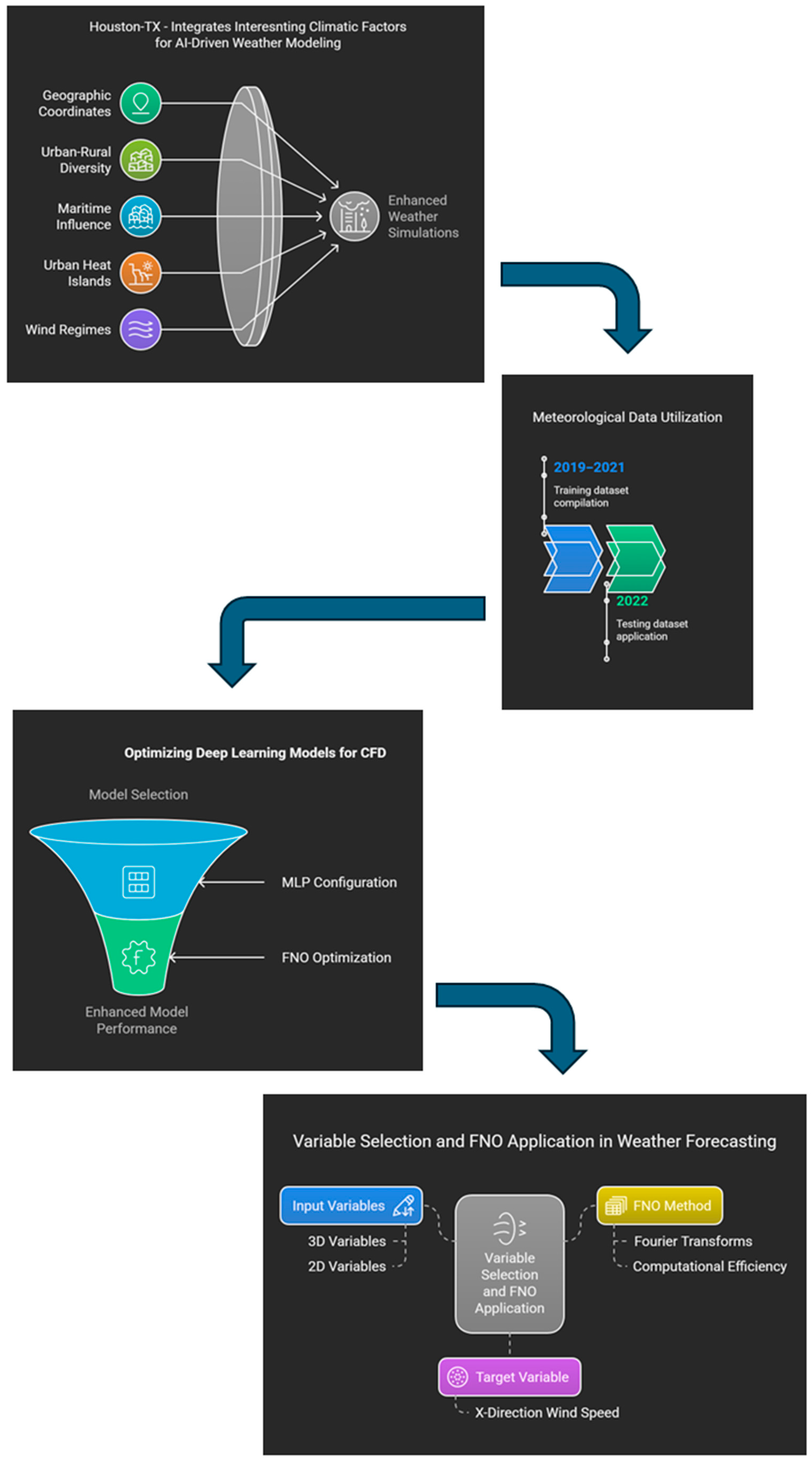
Physics-informed neural networks (PINNs) are a class of deep learning approaches that aim to merge physical laws into neural network architectures for solving partial differential equations (PDEs). Unlike traditional deep learning models, PINNs use mechanisms to induce predictions to adhere to governing equations, targeting accuracy and generalizability, particularly with limited data. PINNs provide an efficient alternative to computationally expensive numerical methods, making them suitable for inverse problems and high-dimensional PDEs [33]. Recent research reports PINNs’ success in fluid mechanics, heat transfer, and materials science, working on improving their capability to reconstruct velocity fields and model stress-strain relationships. PINN frameworks could even outperform experimental correlations and other data-driven methods, providing more reliable predictions in complex physical systems [34].

However, challenges such as spectral bias and optimization difficulties persist. Despite their good results, PINNs are commonly developed in ad hoc situations, thus requiring a specifically developed architecture and weights for each problem. Strategies like adaptive loss weighting and hybrid approaches are being explored to enhance performance [35]. Under this ecosystem, the neural operators are developed to solve classes of ODEs/PDEs promptly. Pre-trained neural operators can also serve as surrogates to represent the physical relationships in addressing hybrid problems. This capability is regarded as one of the major functions of neural operators in the literature since they mimic the physical representation of each one of the parcels of a PDE.

Nevertheless, there is always an inherent set of different noises in PINN solution development, which is probably caused by the nature of neural networks [36]. As statistical models, they tend to “blur” the solution as the optimization process progresses, potentially impacting accuracy [37]. The baseline PINN has been noted to struggle with convergence and accuracy when solving “stiff” PDEs. Addressing this limitation, the Self-Adaptive PINNs (SA-PINNs), a fundamentally new approach to train PINNs adaptively, have been introduced. This methodology dynamically adjusts the training process to enhance both stability and accuracy.

The L² physics-informed loss is the prevailing standard for training PINNs, commonly employed alongside additional loss terms that enforce compliance with fundamental physical laws, such as mass and energy conservation. However, this approach poses challenges due to the complex interplay between the overall loss function and the fidelity of the learned solution. PINNs often exhibit a smoothing effect, as the imposed physics-based constraints mitigate but do not eliminate deviations from physical consistency. In conventional computational fluid dynamics (CFD) simulations, users explicitly define error thresholds to establish convergence criteria, ensuring controlled numerical accuracy. In contrast, neural network-based approaches lack an equivalent mechanism for precisely defining stopping conditions, complicating their integration into traditional numerical frameworks. Although PINNs have not yet achieved the same level of accuracy and reliability as CFD solvers for general problem-solving, their incorporation into numerical simulations presents promising opportunities. This study investigates the potential of utilizing PINNs to enhance the initialization of transient CFD simulations, aiming to improve computational efficiency and accelerate convergence.

3. Methodology

3.1. The Study Area

The study area is geographically located between the latitude coordinates 28.180214° N and 31.322086° N and the longitude coordinates 97.1828° W and 93.5202° W, encompassing the city of Houston, Texas, and its surrounding regions. This area includes both urban and rural landscapes, offering a diverse range of environmental and climatic conditions for investigation [38,39]. The region under investigation is depicted in Figure 1.

The proximity of Houston to the Gulf of Mexico makes the region particularly influenced by maritime weather systems, such as hurricanes, intense convective activity, and high humidity levels [41,42]. The city’s dense urban infrastructure also creates localized phenomena, such as urban heat islands, which interact with broader atmospheric dynamics [43,44]. The region is characterized by complex wind regimes shaped by coastal and inland influences. These include consistent southeasterly winds originating from the Gulf of Mexico, which dominate much of the year, as well as periodic shifts driven by frontal systems and cyclonic activity [45]. These variable wind patterns significantly affect local weather, pollutant dispersion, and energy resource management, making them a critical factor in this study [46,47,48,49].

Selecting this region offers an opportunity to test and validate the use of artificial intelligence tools for improving initial conditions in transient CFD-based meteorological models like WRF. By focusing on a geographically and climatically dynamic area with intricate wind regimes, the study aims to enhance weather simulations’ computational efficiency and accuracy, particularly in scenarios involving rapidly evolving weather systems. In this sense, with the fact that this is a proof of concept study in mind, we opted to focus on this specific region to make the conclusions presented here clearer.

3.2. Data Specifications and Variable Definitions

The study utilizes high-resolution meteorological data generated by the WRF model, obtained directly by running the code by our team. The dataset is divided into two periods to facilitate the training and testing of the proposed methodologies. The dataset has a time resolution of 1 h.

The training dataset comprises WRF simulation outputs spanning three years, from 2019 to 2021. This dataset captures a wide range of atmospheric conditions, including seasonal variations, extreme weather events, and changes in local wind regimes, aiming for a robust training process. Including several predictive parameters in WRF simulations is often beneficial, deeming the model capable of generalizing across diverse scenarios [46,50].

For testing purposes, the study employed WRF simulation data from 2022. This separated dataset allows for an independent evaluation of the proposed methods, ensuring that the results accurately reflect the model’s ability to predict future conditions without bias from the training data [51,52]. The time used here was primarily based on memory requirements to run the simulations. Secondly, even though it is not the direct scope of this study, we tried to be inside the time range where the field data is available for Houston and potentially may be used in future works for further validation. Furthermore, the use of a whole year (2022) provided a way to check the performance for all the different weather regimes that happen during all the seasons.

WRF output files contain numerous meteorological and environmental variables, including 2D surface fields and 3D atmospheric profiles. The variables were limited to a shorter list of key 2D and 3D attributes (

Table 1. List of 2D variables present in the WRF simulations and used in the variable selection process. “Times” is a 1D variable, but it is inserted here for the sake of space.

WRF Name	Units	Description
“Times”	hh:mm:ss	Time
“XLAT”	degree	Latitude of the collocated grid
“XLONG”	degree	Latitude of the collocated grid
“XLAT_U”	degree	Latitude of the staggered grid in the X direction
“XLONG_U”	degree	Longitude of the staggered grid in the X direction
“XLAT_V”	degree	Latitude of the staggered grid in the Y direction
“XLONG_V”	degree	Longitude of the staggered grid in the Y direction
“COSZEN”	degree	Cosine of the zenith angle of the Sun
“PSFC”	Pa	Surface pressure
“T2”	K	2-m temperature
“Q2”	kg water vapor/kg air	2-m specific humidity
“U10”	m/s	10-m U-component of wind
“V10”	m/s	10-m V-component of wind
“SST”	K	Sea surface temperature
“TSK”	K	Skin temperature
“TSLB”	K	Soil temperature at specified layers
“HGT”	m	Geopotential height
“ALBEDO”	Fraction (0-1)	Surface albedo

and

Table 2. List of 3D variables present in the WRF simulations and used in the variable selection process.

WRF Name	Units	Description
“U”	m/s	U-component of wind
“V”	m/s	V-component of wind
“W”	m/s	W-component of wind
“T”	K	Air temperature
“THM”	K	Moist potential temperature
“QVAPOR”	kg water/kg dry air	Water vapor mixing ration
“QCLOUD”	kg water/kg air	Cloud water mixing ration
“QRAIN”	kg rainwater/kg air	Rainwater mixing ratio
“P”	Pa	Perturbation pressure
“P_HYD”	Pa	Hydrostatic pressure
“PB”	Pa	Perturbation base-state pressure

) to streamline the analysis and maintain consistency with the simulations. In fact, all the variables present in the WRF output files were tested. This set of variables is an intrinsic characteristic of WRF’s runs and, thus, not controlled by the authors. This focused selection ensures that the inputs used in the AI-based initialization are directly aligned with those employed in the actual WRF simulations. This improves the computational efficiency and preserves the critical information needed for accurate predictions.

The latitude–longitude data and wind speed components (U, V, and W) were always included as inputs for all developed models. Additional auxiliary variables were tested separately to evaluate their impact on the performance of the models. The target variable for prediction was maintained consistently throughout this work as the X-direction wind speed component, ‘U’, reflecting the proof-of-concept nature of the study. The aim is to focus on a single output variable, allowing for a more concise and objective presentation and analysis of the results, ensuring clarity and allowing a direct analysis.

This study limited the number of time steps used to predict the next step to two. This choice aligns with the standards applied by Microsoft Aurora and was adopted for computational efficiency and memory usage considerations [53]. The approach balances predictive accuracy with resource constraints by leveraging a minimal yet effective input size, making it feasible for operational meteorological applications.

Including hourly resolution data, using two time-steps, consistent use of wind and spatial variables, and reduced/optimized variable set to ensure that both short-term and long-term atmospheric phenomena are accurately represented. These decisions collectively aim to enhance the reliability of the proposed techniques while maintaining the computational efficiency necessary for transient CFD models like WRF.

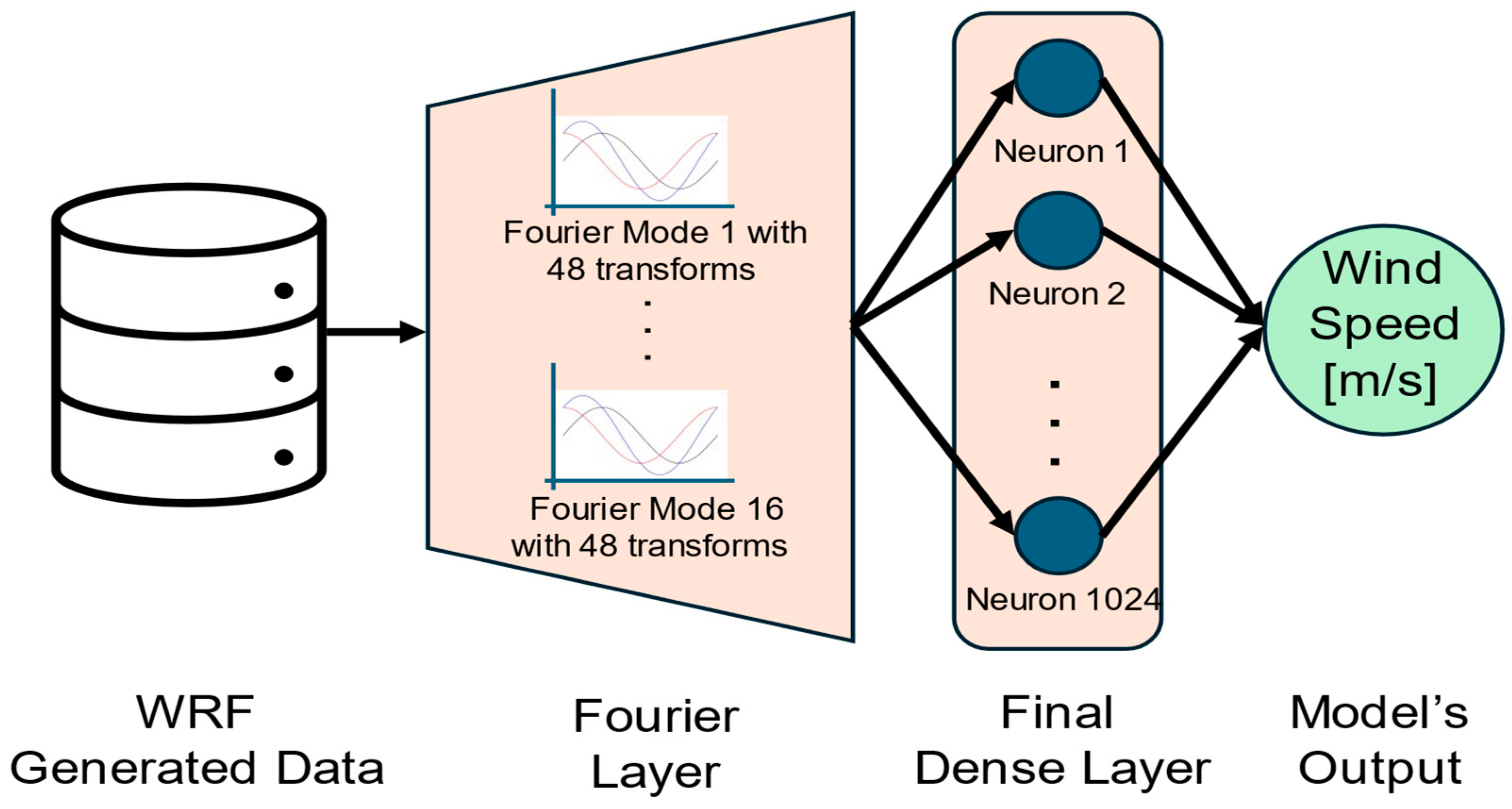
3.3. Applied Deep Learning Models

To evaluate the feasibility of using artificial intelligence to improve the initialization process of transient CFD models, two distinct deep learning architectures were tested: a multilayer perceptron (MLP) network and a Fourier neural operator (FNO) network. Each model was chosen for its capabilities to address the specific comparisons carried out in this work.

The multilayer perceptron (MLP) is a feedforward neural network where every neuron in one layer is connected to every neuron in the next layer. It is well-regarded for its simplicity and versatility in learning structured datasets, and it is theorized to serve as a universal function approximator [54]. An incremental approach of the hyperparameters was adopted to determine an optimal configuration. Initially, a zero hidden layer architecture was tested, where the network consisted only of an input layer and an output layer, providing a baseline for direct input-output mapping. Subsequently, the number of neurons in the input and output layers was varied. The best performance was achieved with 1024 neurons.

Once this configuration was established, the number of hidden layers was tested while freezing the number of neurons at 1024 per layer. The results revealed that the best outcomes on the testing dataset occurred when the network had 0 hidden layers, confirming that a shallow network was sufficient to capture the link between the inputs and the target variable (U, the X-axis component of wind velocity). For this setup, the root mean squared error (RMSE) for the testing set was 4.7551 m/s. While this result served as a useful baseline, it will be shown that the FNO significantly outperformed the MLP, demonstrating its suitability for the complex spatiotemporal patterns inherent to the WRF dataset.

The FNO represents a more advanced methodology tailored for learning operators in PDEs. Unlike traditional neural networks, the FNO models the solution operator, allowing it to predict also multiple instances simultaneously [28]. This property makes FNO highly generalizable and capable of capturing a broader range of solution cases, as it is not constrained to a specific instance or condition. In fact, FNO has recently been applied quite successfully in the development of DL solutions for differential equations. However, its use has been evaluated mainly in equations that, despite being very relevant, are famous for having a strong theoretical appeal, as this facilitates obtaining references for benchmarking. This research effort is relevant as it indicates the suitability of FNO for this type of problem. This fact was one of the reasons that motivated us to use it for our proof of concept, which ended up showing how feasible the proposed approach can be. In this sense, in our study, this feature was leveraged by training and testing the FNO across a variety of conditions.

The FNO’s hyperparameters were optimized over two rounds (no more than that was needed), where the following parameters were systematically tested in sequence:

• The size of the final hidden layer;
• The number of Fourier modes, in powers of 2 (from 1 to 16);
• The width, defined as the number of transforms applied to the Fourier modes;
• The number of stacked Fourier layers, also in powers of 2 (from 1 to 16).

Via this iterative optimization process, the best architecture was found to have 1024 neurons in the final hidden layer, 16 Fourier modes, a width of 48, and only one Fourier layer. This configuration achieved a final testing RMSE of 1.2544 m/s, showcasing a significant improvement over the MLP model. The schematics of the used FNO architecture is presented in Figure 2.

For this step, the choice of input variables is aimed at maintaining the physical consistency of the system. We started with variables considered relevant to the underlying physics, and the initial dataset was limited to the following:

• 3D variables: U, V, and W (wind speed components in X, Y, and Z directions) and T (temperature);
• 2D variables: latitude–longitude, while U10 and V10 (wind speed components at 10 m above the surface) were used to provide information on surface conditions.

The presented selected auxiliary variables were used as inputs, while the target variable was the X-direction wind speed component (U). The decision to predict a single output variable was to make results more concise since the results obtained are intended to be proof of concept, which can be expanded later to a complete weather forecasting application.

The FNO’s reliance on Fourier transforms enables it to efficiently model spatial and temporal interactions, making it particularly well-suited for the distributed and transient nature of WRF data. The results highlight the FNO’s potential to reduce computational costs and enhance numerical weather prediction systems by accelerating the convergence of transient CFD models.

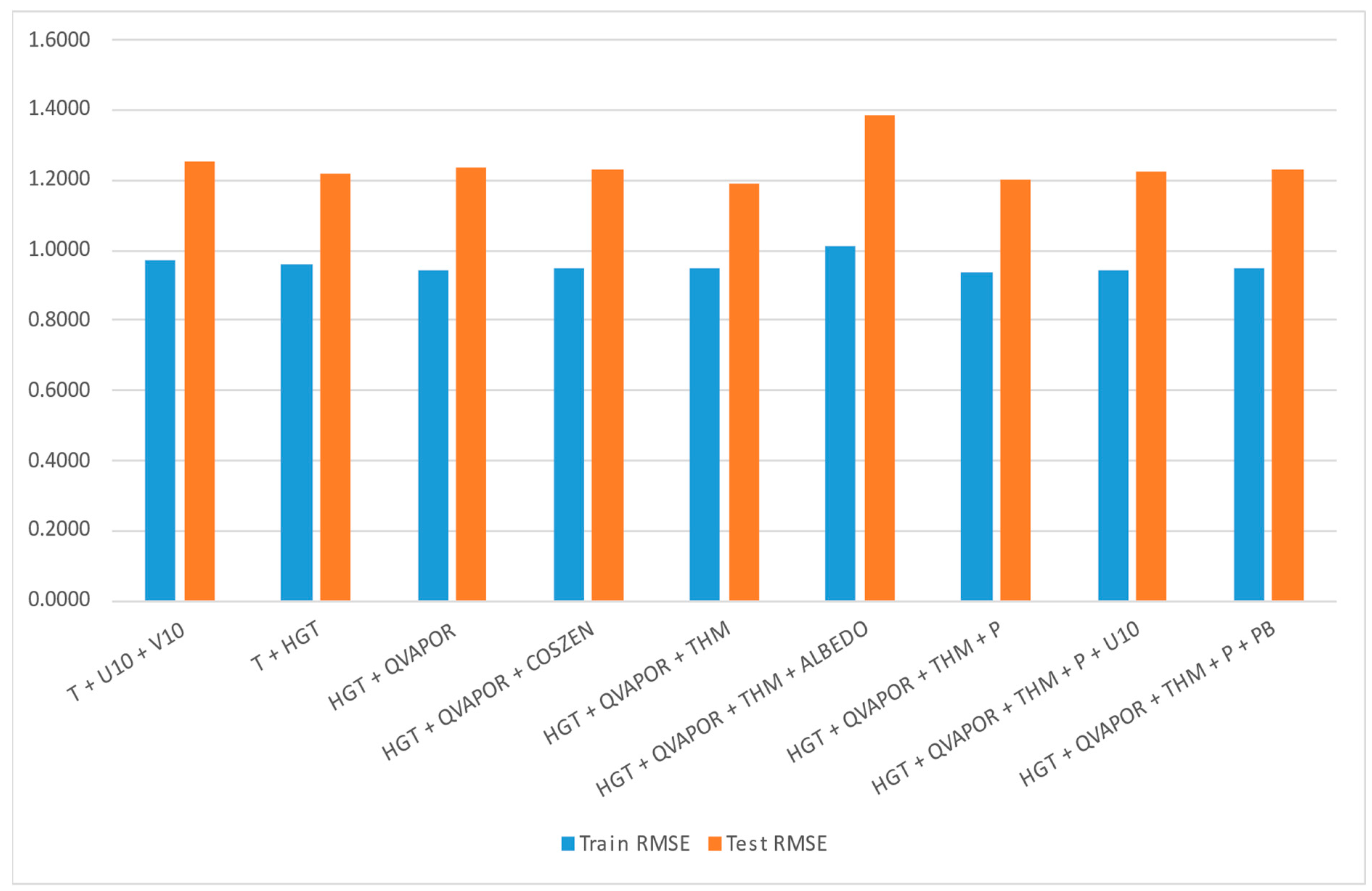
3.4. Variable Selection

In this study, the initial approach to variable selection involved applying a single model across all Z-levels, encompassing and predicting all vertical layers in the dataset, what we call here and throughout the remainder of this manuscript “the global model”. However, as it will be demonstrated later, this approach can be modified and enhanced by using one model per reference height, totaling 34 individual height levels. This adjustment aligns with the distinct atmospheric conditions at different altitudes and allows for a more tailored and precise modeling approach.

The initial variable set used in the modeling process included U, V, and W (wind speed components in the x-easting, y-northing, and z-elevation directions), T (temperature), and U10 and V10 (wind speed components at 10 m above ground level). This selection is consistent with the variables chosen for the FNO model discussed in the previous subsection.

A systematic, iterative process was implemented to refine the input variables and enhance prediction accuracy. In each round of testing, all available variables from the dataset (but U, V, and W, and latitude–longitude, which were always kept) were considered as potential substitutes for the original set. The process alternated between testing only 2D variables (e.g., surface variables) and testing only 3D variables (e.g., variables across vertical layers).

The two-dimensional (2D) variables’ surface-specific characteristics often result in minimal coupling with higher-altitude atmospheric dynamics. Consequently, if the inclusion of a given 2D variable in an iteration failed to yield a contraction in the RMSE, it was systematically excluded from subsequent training rounds to optimize model performance. In contrast, three-dimensional (3D) variables were retained across all iterations, as their incorporation consistently led to RMSE improvements. This persistent enhancement underscores the critical role of vertical atmospheric profiling in accurately resolving the physical mechanisms governing wind flow dynamics within the computational fluid dynamics (CFD) framework.

Finally, the variable set comprising HGT (height, 2D), QVAPOR (water vapor mixing ratio, 3D), and THM (perturbed moist potential temperature, 3D) emerged as the best-performing set for the case of using a single model across all Z-levels. This selection highlighted the relevance of combining surface and vertical atmospheric variables to represent the physical conditions affecting wind flow accurately.

The selection rounds continued until no further improvement was observed in the testing RMSE. This iterative optimization allowed us to determine the most relevant variables for predicting the target output, ensuring that unnecessary inputs were excluded and that computational efficiency was maintained (Figure 3).

This methodology (condensely presented in Figure 4) aimed to underscore the importance of variable selection in reducing model complexity and improving prediction accuracy using the lowest computer resources. The transition from a universal model across all Z-levels to individualized models per height, combined with an optimized variable set, presented in the next section, forms the foundation for the enhanced results presented in this study.

4. Results and Discussion

4.1. Global Model Performance

To assess the overall accuracy of the proposed approach, the performance of the global model, which simultaneously utilizes and predicts variables across all z-levels, was evaluated using a normalized metric. The RMSE values were normalized by dividing them by the average absolute value of the U velocity component across the entire domain [51]. This normalization facilitates a clearer interpretation of the model’s performance by providing a relative measure of error magnitude concerning the predicted variable.

$$nRMSE={\displaystyle \frac{RMSE}{\frac{{\sum }_i^n\left|U_i\right|}{n} }}$$

(1)

The resulting normalized RMSE (nRMSE) for the global model was 17.15%, indicating the percentage deviation from the expected values. In contrast, the persistence model, which represents the baseline approach commonly used in all CFD transient algorithms (e.g., [55,56]), where the velocity field of the previous time step is directly applied to the next step, achieved a lower nRMSE of 13.69% for the entire 3D domain. This can be explained in a somewhat straightforward way since the global model has to cope with data from several Z-levels simultaneously, which leads the model training process to seek an ‘average’ solution that approximates the global values of the atmosphere. The persistence model, despite its simplicity, by definition, uses values from the same Z-level, which already gives it a local focus.

To confirm, the performance of the global model was further analyzed at three specific Z-levels: 0 (surface), 16 (middle atmosphere), and 33 (top of atmosphere). The results indicated that the global model did not outperform the persistence approach at any of these levels. At Z-level 0 (surface), the global model’s normalized root mean squared error (nRMSE) was 41.93%, whereas the persistence model achieved a lower error of 33.37%. The increased error at the surface is likely attributed to strong gradients caused by irregular terrain, boundary layer effects, and additional constraints imposed by empirical models used to approximate surface interactions, all of which introduce further uncertainties [54].

At Z-level = 16 (middle atmosphere), the nRMSE was 29.84%, while the persistence approach achieved 26.55%. The results at this altitude are closer between the two models, probably because the atmosphere becomes more predictable and stable, reducing variability and making persistence a more practical approach [57].

Finally, at Z-level = 33 (top of atmosphere), the nRMSE was 12.30%, whereas the persistence model reached a significantly lower 6.32%. Even though the global model improved its performance at this height due to the more stable atmospheric conditions, it still did not outperform the persistence model. Furthermore, the improvement observed for the global model at this level was not as significant as at the lower levels, leaving its error almost twice as large as that of persistence.

The results obtained indicate that a single global model does not outperform the persistence model, at least for the optimized FNO model. This suggests that the current approach may not fully capture the dynamics of the atmosphere at different heights simultaneously. Some factors may detail the reasoning behind these results:

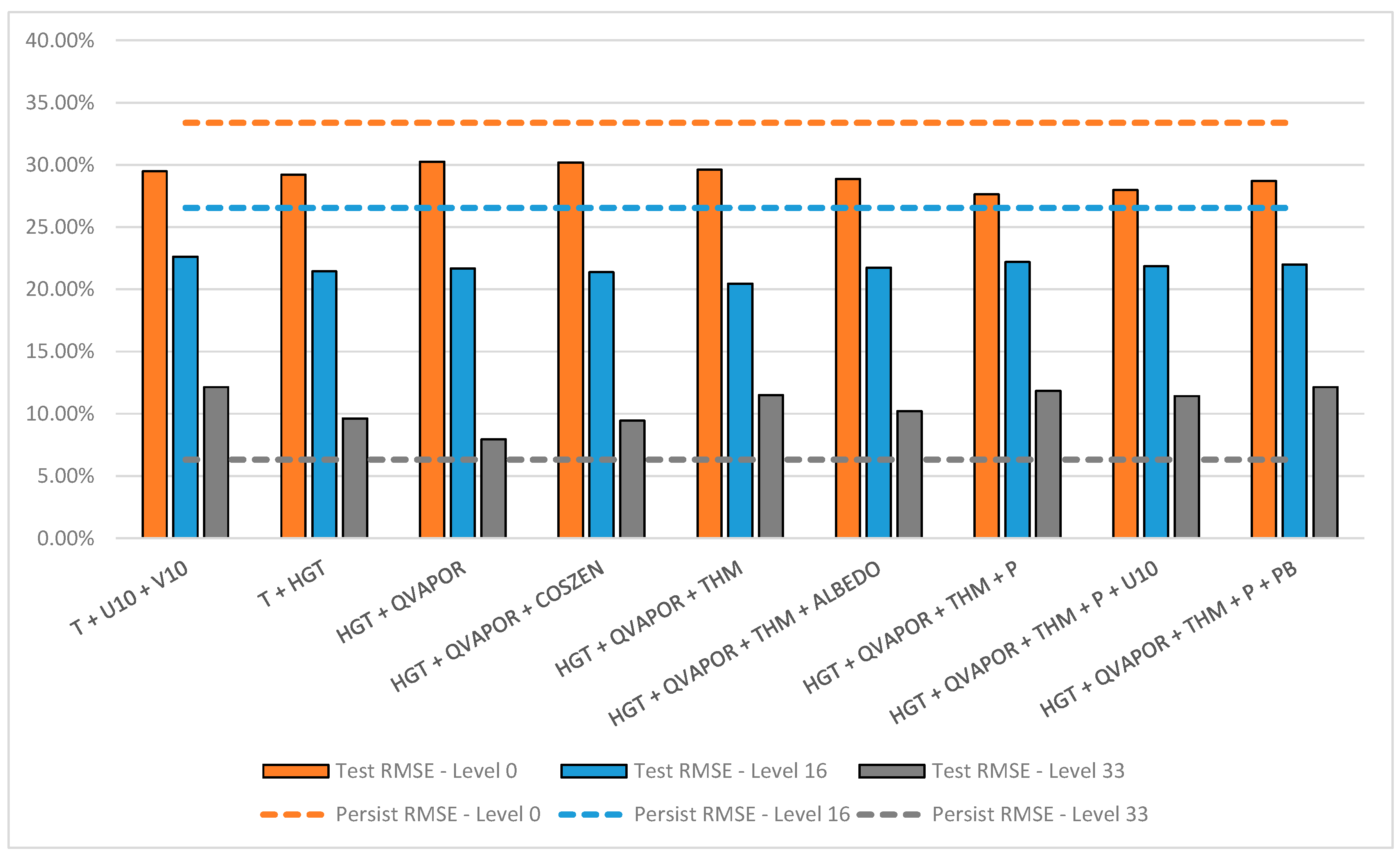
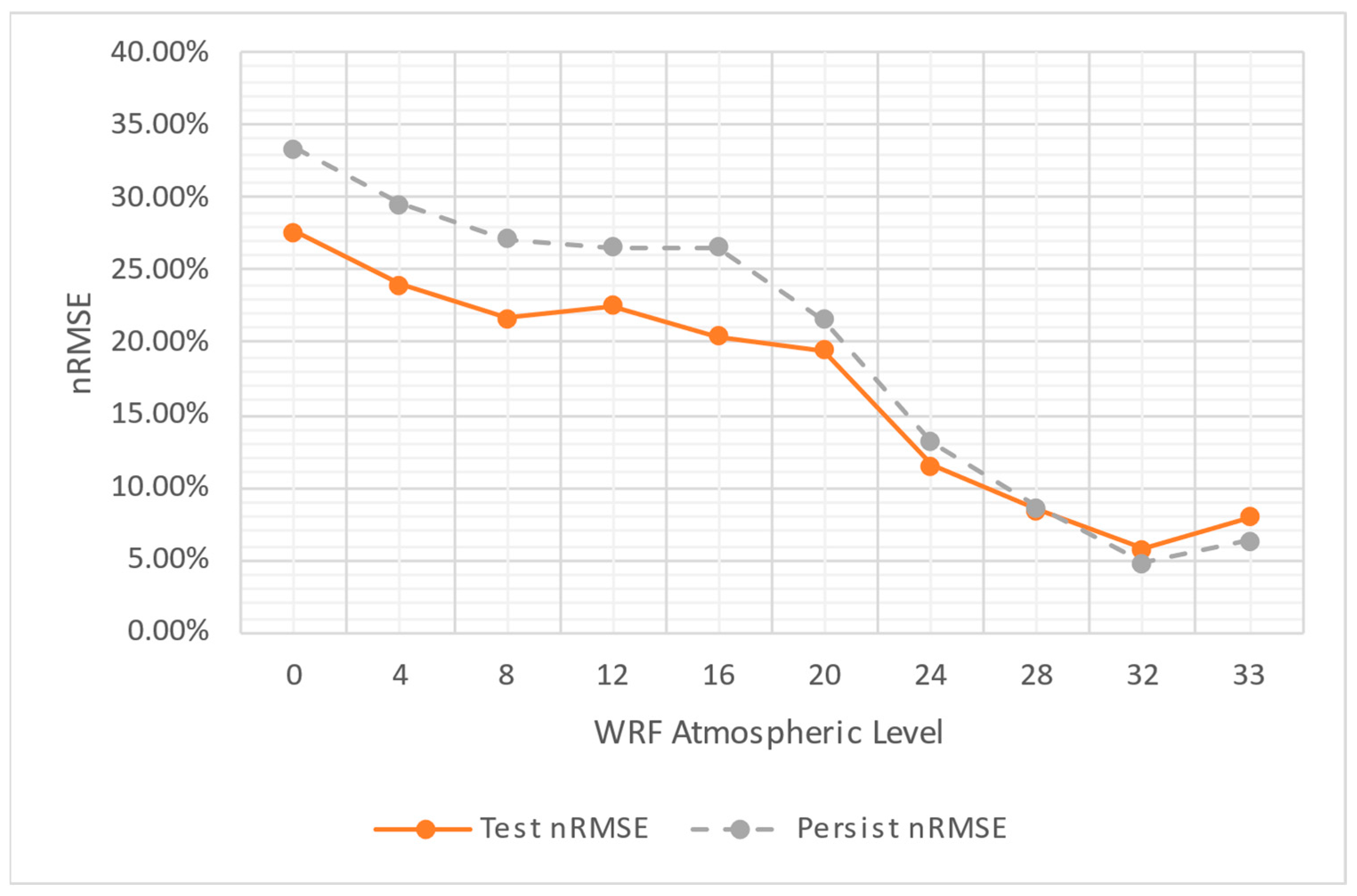
• Lack of height-specific modeling: The persistence model benefits from the natural continuity of the atmospheric flow, whereas the deep learning model needs to generalize across all heights. Studies such as [58] suggest that stratified modeling can significantly enhance predictive performance, where different models are trained for different atmospheric layers.
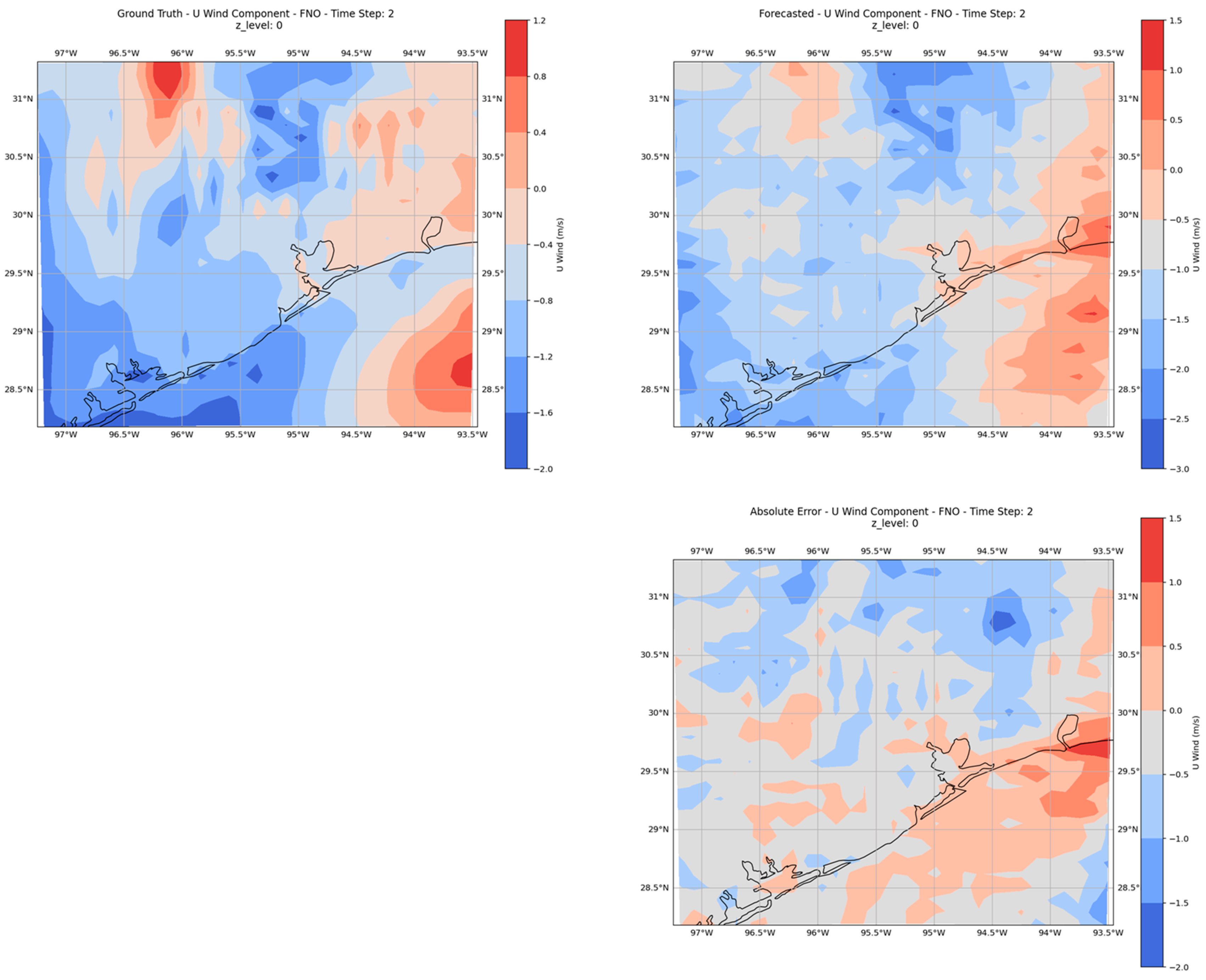
• Boundary layer effects: Near-surface wind flows are influenced by topography, land use, and temperature variations, which cause strong local gradients and turbulence [59]. The inability of the global model to properly learn these effects might be a reason why it underperformed compared to persistence at Z-level 0.
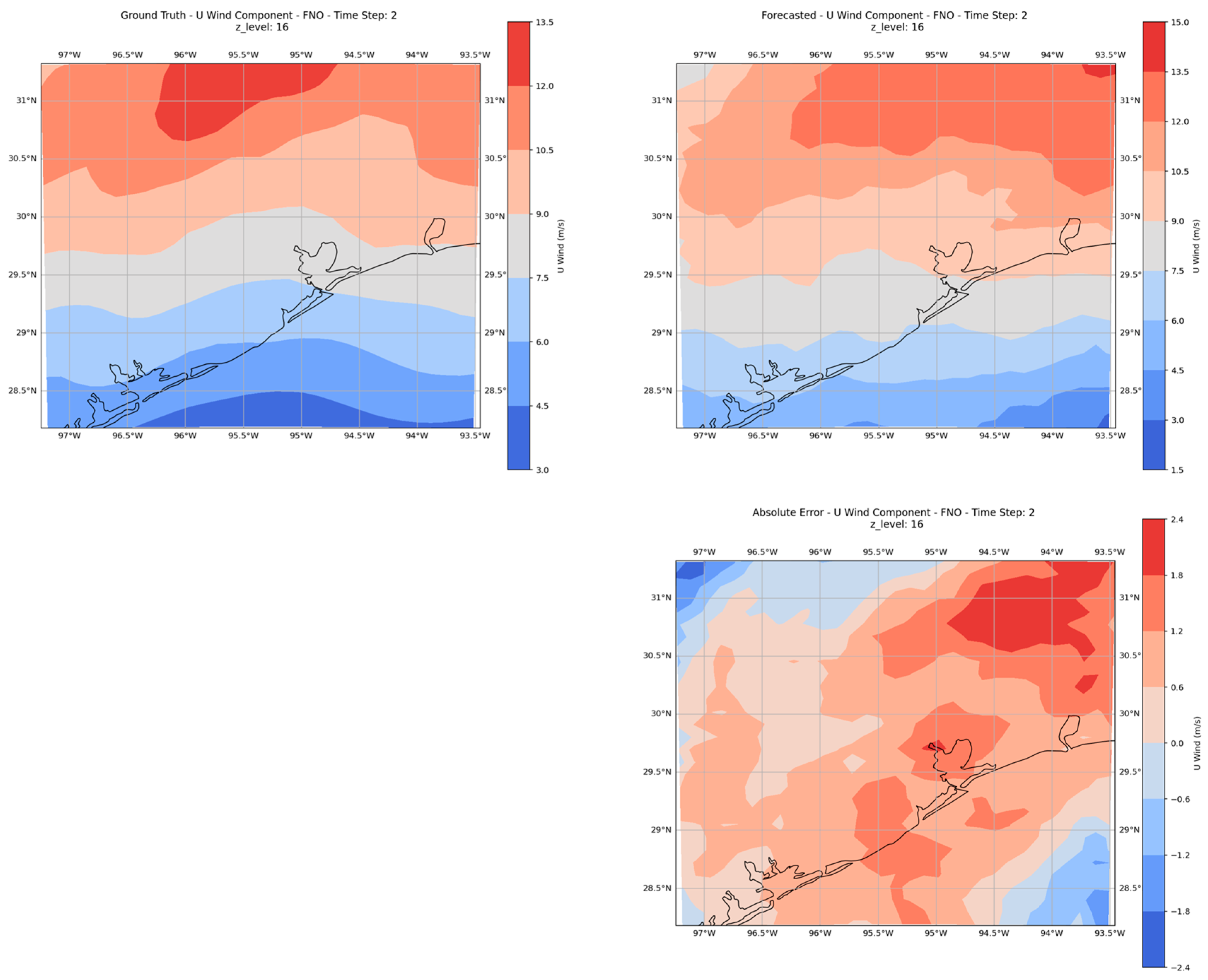
• Predictability of atmospheric layers: The results at Z-level = 16 show that the atmosphere is more predictable at mid-altitudes, which aligns with previous findings that suggest lower turbulence and more stable wind regimes at these heights [60]. This explains why persistence and the global model performed similarly.
• Impact of training data and physical constraints: The FNO model was trained using PINN principles, yet its ability to fully integrate the governing physics of the atmosphere might still be limited compared to conventional numerical weather prediction (NWP) models. Hybrid approaches that combine FNO architectures with physics-based constraints have shown promise in recent literature [61].

These findings reinforce the need to refine our methodology. A promising alternative would be to apply height-dependent models, where a different FNO network is trained for each height level, ensuring that each model learns the specific characteristics of wind dynamics at its respective altitude. This will be further explored in the next section.

4.2. Specific Z-Levels Ad Hoc Models

This section presents the results of training separate models for each Z-level, which significantly improved performance compared to using a single global model for the entire 3D domain. The specialized models outperformed persistence for both the surface (Z = 0) and middle atmosphere (Z = 16). In contrast, at the top of the atmosphere (Z = 33), the results were slightly worse than persistence but still highly competitive.

Figure 5 illustrates these findings, highlighting the impact of height-specific modeling. For the surface level (Z = 0), the optimized FNO model achieved an nRMSE of 27.64%, outperforming the persistence model, which yielded 33.37%. The best-performing variable set for this level consisted of “HGT”, “QVAPOR”, “THM”, and “P”. At the middle atmosphere (Z = 16), the FNO model further improved over persistence, with an nRMSE of 20.46% compared to 26.55%, using the variables “HGT”, “QVAPOR”, and “THM”. At the top of the atmosphere (Z = 33), the nRMSE was 7.95% for FNO, while persistence performed slightly better at 6.32%, with the best variable set comprising only “HGT” and “QVAPOR”.

It can be perceived that variables with a strong physical appeal, which indicate either concrete physical characteristics (“HGT”) or significant portions of physical balances (“QVAPOR”, “THM”) or even thermodynamic correlations (“THM”, “P”), have shown to pursue a strong impact, as they provide concrete information about atmospheric dynamics. Variables that are correlated to these tended not to improve the results. This leads us to infer that they are useful in the WRF model to determine more subtle local/temporal variations but that in the DL paradigm, they may function as autocorrelated predictors.

DL models are highly capable of finding subtle relationships between variables as long as the most appropriate ones are selected. This reiterates the good performance of models developed specifically for each Z-level.

Even though this is a proof of concept, and having in mind that the purpose was to verify the ability of DL models to be used as surrogates for the initial iteration of a transient CFD process, the interpretation of the results can be extended, especially to extreme conditions and more complex regions. This is because, since the best performance gains were achieved in the most challenging situations, from the mid-atmosphere to the surface, it can be inferred that the proposed approach has a high potential to be successful in more adverse situations.

These results align with previous atmospheric modeling and machine learning findings for weather prediction. Some authors emphasize that near-surface wind prediction is particularly challenging due to the influence of orography, boundary layer turbulence, and localized surface conditions [62,63]. The improvement seen at Z = 0 with the ad hoc model can be attributed to better handling of these complex near-surface interactions, as the inclusion of pressure (P) appears to have contributed to refining the model’s predictions. In contrast, at Z = 16, the atmosphere is already more stable, which reduces the impact of localized disturbances, making the FNO model even more effective.

At the top of the atmosphere, the slight underperformance compared to persistence suggests that the model is not yet fully capturing the larger-scale atmospheric dynamics that dominate at these heights. However, the small difference in error indicates that the FNO approach remains competitive. Similar findings have been reported by [31], who showed that machine learning models tend to struggle with upper-atmosphere predictions unless explicitly trained with large-scale flow features.

Another key insight from this analysis is that, as altitude increases, fewer variables are needed to achieve optimal results. This observation is probably due to the atmosphere’s increased stability and the lower influence of complex terrain interactions at higher altitudes. This trend is consistent with studies on numerical weather prediction, which indicate that lower atmospheric levels require more detailed parameterizations due to their interaction with the Earth’s surface, while higher-altitude predictions benefit primarily from large-scale flow patterns [64].

Overall, the results confirm that height-specific modeling provides a significant advantage in transient wind field predictions. The FNO-based approach, when applied separately for each Z-level, successfully reduced prediction errors and demonstrated strong potential for improving atmospheric simulations over conventional persistence models.

Figure 6, Figure 7 and Figure 8 illustrate the case of a specific time step for each studied Z-level (respectively 0, 16, and 33). It visually assesses the FNO model’s performance at distinct altitudes. As observed, the model’s accuracy improves with increasing height, aligning with findings from similar studies. Nevertheless, it can be seen how the color patterns of the modeled fields properly reproduce the ground truth pattern.

To close the comparison, Figure 9 illustrates the variation of the nRMSE across the WRF atmospheric levels, comparing the performance of the persistence model with the ad hoc models developed for each level. The results indicate that the ad hoc models consistently outperform the persistence approach from the surface up to the mid-atmosphere. Beyond level 20, the performance of both approaches becomes comparable, and at the top of the atmosphere, the discrepancies are negligible. The proposed methodology is particularly advantageous as it significantly reduces the error in most of the atmosphere, especially in regions with more intense variations, where CFD models will have a higher computational load to achieve convergence. This further highlights the importance of employing the developed models instead of relying on a simple persistence approach.

Similar results may be found in the literature. For instance, in [65], the FNO model demonstrated varying performance across distinct urban layouts and wind scenarios. While the results indicated that the FNO model could offer accurate prediction and achieve a remarkable 99% reduction in the required computational time, its ability to generalize to new wind directions proved challenging. This suggests that the FNO model’s performance is shaped by the complexity of the environment and the specific conditions under which it is applied.

Similarly, in [66], the authors investigated the application of machine learning models to predict wind speeds at higher altitudes based on data from lower levels. Their findings revealed that wind speed values at higher altitudes are directly influenced by the corresponding value at lower altitudes for the same geographical location. This indicates that machine learning models can adequately capture altitude-dependent relationships, leading to accurate predictions at higher levels.

These studies show that the FNO model’s performance improves with altitude, likely due to the decreasing complexity and increased predictability of atmospheric conditions at higher levels. The visual evidence provided in Figure 5 underscores this trend, highlighting the model’s enhanced accuracy as height increases.

Other studies have shown the feasibility of Fourier-based approaches for atmospheric modeling. The model proposed by Pathak et al. [67] was built upon a Fourier neural network, used reanalysis data from the ERA5 dataset for training and validation, and successfully predicted wind speed for both land and sea regions. Unlike our study, however, their work found that increasing the number of attributes returned improved results by the model. This might be attributed to the fact that their model seeks a more general approach than ours and would benefit further from more spatiotemporal information provided by the input attributes. Contrarywise, the ad hoc models proposed in our study are tailored for specific atmospheric interactions, thus requiring different input attributes for each scenario, as the scenario’s complexity decreases with higher altitudes.

In another study [68], the authors developed the Local-FNO model for modeling the microclimate of their study site. Their results highlighted that the model using local information for the location reached better outcomes than the vanilla FNO approach for wind dynamics modeling for different building geometries. Their findings corroborate the superior efficiency of the ad hoc methodologies presented in this work on capturing local patterns.

The following

Table 3. Literature found work for atmospheric modeling using ML.

Model	Methodology	References
FNO	Implementation of an FNO model for forecasting wind in different urban configurations and wind scenarios	[65]
Support Vector Machine, K-Nearest Neighbor, and Gradient Boosting Machine	Implementation of different traditional machine learning approaches for wind speed forecasting using data collected from different altitudes.	[66]
FourCastNet	Implementation of a Fourier-based approach to forecast atmospheric variables, including wind speed, precipitation, and water vapor, using deep learning.	[67]
Local-FNO	Precise modeling of urban microclimates, including wind velocity and temperature.	[68]

compiles the works of the literature found that are related to the present study.

5. Conclusions

This study developed and investigated a proof of concept on applying deep learning techniques for wind speed prediction using a Fourier neural operator (FNO) and a multilayer perceptron (MLP). The models were trained and tested with WRF-generated data for Houston from 2018 to 2022, focusing on predicting the X-direction wind speed component. The MLP was used primarily as a baseline, achieving a testing RMSE of 4.75 m/s, while the optimized FNO significantly outperformed it, reducing the RMSE to 1.25 m/s.

We initially trained a single global model across all Z-levels, which, despite its advanced architecture, still did not outperform the persistence model for wind prediction. Normalized RMSE values revealed that the global model reached an nRMSE of 17.15%, compared to 13.69% for the persistence model.

To improve upon these results, we implemented and tested Z-level-specific models, significantly enhancing the performance at lower altitudes. At the surface (Z = 0), our optimized FNO model achieved an nRMSE of 27.64%, outperforming persistence at 33.37%. In the middle atmosphere (Z = 16), the nRMSE improved to 20.46%, compared to 26.55% for persistence. For the top of the atmosphere (Z = 33), although persistence still outperformed our model (6.32% vs. 7.95%), the results remained highly competitive, which can help implement a fully automated process. This process shall benefit from using the model output to start the iterative process of the transient CFD solution, which is slow and has a high computational demand. This will require fewer iterations, optimizing processing time and its associated financial costs.

Variable selection played a relevant role in model optimization. While all models always used latitude-longitude data and wind components, we tested auxiliary variables to pinpoint the most pertinent attributes for each height. The optimal feature sets varied across Z-levels, suggesting that different physical phenomena dominate wind behavior at different heights. At lower levels, the inclusion of HGT, QVAPOR, THM, and pressure yielded the best results, while higher-altitude models required fewer input variables, likely due to the increasing stability of the atmosphere.

The study case provided visual confirmation of model performance, reinforcing that FNO’s effectiveness improves with altitude. This aligns with previous studies demonstrating that machine learning-based wind forecasting benefits from stratifying models based on atmospheric layers.

A key takeaway from this study is the potential of the FNO model to learn complex spatial and temporal dependencies in atmospheric fields, offering a data-driven alternative to conventional numerical simulations. The findings also underscore the importance of tailoring machine learning architectures and input features to the specific atmospheric characteristics at different altitude levels.

Despite these promising results that validate the proof of concept, integrating the FNO model into operational weather forecasting systems presents challenges. A major issue is the computational cost of training deep learning models on large-scale meteorological datasets. Although inference times are significantly faster than those of traditional numerical models, the requirement for high-performance computing infrastructure may pose a barrier. Furthermore, ensuring the model’s generalization across diverse weather conditions involves continuous data assimilation and periodic retraining with updated datasets. Possible solutions include hybrid approaches that combine physics-based simulations with deep learning predictions, the application of transfer learning to adapt pre-trained models to various climate regimes, and utilizing cloud-based infrastructures to efficiently scale computational resources. Addressing these challenges will be essential to unlocking the full potential of deep learning for atmospheric modeling and real-time forecasting applications.

While the FNO model shows promise, it has limitations that must be considered for broader applicability. One key challenge is its ability to accurately predict extreme weather events, which often involve highly nonlinear dynamics and rapid atmospheric changes that may not be well captured by the learned solution operator. Additionally, the model’s performance in regions with complex topography remains a concern, as steep terrain can introduce strong local gradients and boundary effects that require high-resolution input data and specialized handling. Future work should focus on enhancing the model’s robustness through techniques such as adaptive resolution strategies, hybrid physics-informed approaches, and the incorporation of additional observational data to improve predictive accuracy in these challenging scenarios.

Overall, this research highlights the potential of deep learning for atmospheric forecasting, emphasizing the need for height-specific models. Future work may explore extending the findings presented here by applying our approach to other variables. Furthermore, hybrid methods that combine deep learning with domain-specific physics constraints may be tested, along with extending the methodology to more diverse atmospheric conditions and locations.

Finally, the results indicate the feasibility of using DL models to start the transient CFD iterative process. Once this possibility is demonstrated, additional tests can be performed to quantitatively evaluate the computational costs of this solution, which, due to its scope and implementation complexity, becomes a potential research object. This type of result has the potential to lead to cheaper and faster weather simulations, which is a pressing demand in our modern society.

References

1. Cabrera, D.; Quinteros, M.; Cerrada, M.; Sánchez, R.-V.; Guallpa, M.; Sancho, F.; Li, C. Rainfall Forecasting Using a Bayesian Framework and Long Short-Term Memory Multi-Model Estimation Based on an Hourly Meteorological Monitoring Network. Case of Study: Andean Ecuadorian Tropical City. Earth Sci. Inform. 2023, 16, 1373–1388. [Google Scholar] [CrossRef]
2. Tahir Bahadur, F.; Rasool Shah, S.; Rao Nidamanuri, R. Air Pollution Monitoring, and Modelling: An Overview. Environ. Forensics 2024, 25, 309–336. [Google Scholar] [CrossRef]
3. Roy, C.; Rahman, M.R.; Ghosh, M.K.; Biswas, S. Tropical Cyclone Intensity Forecasting in the Bay of Bengal Using a Biologically Inspired Computational Model. Model. Earth Syst. Environ. 2024, 10, 523–537. [Google Scholar] [CrossRef]
4. Singh, H.; Ang, L.-M.; Lewis, T.; Paudyal, D.; Acuna, M.; Srivastava, P.K.; Srivastava, S.K. Trending and Emerging Prospects of Physics-Based and ML-Based Wildfire Spread Models: A Comprehensive Review. J. For. Res. 2024, 35, 135. [Google Scholar] [CrossRef]
5. Kumar, V.; Sharma, K.V.; Caloiero, T.; Mehta, D.J.; Singh, K. Comprehensive Overview of Flood Modeling Approaches: A Review of Recent Advances. Hydrology 2023, 10, 141. [Google Scholar] [CrossRef]
6. Wu, J.; Wang, Z.; Dong, J.; Cui, X.; Tao, S.; Chen, X. Robust Runoff Prediction with Explainable Artificial Intelligence and Meteorological Variables From Deep Learning Ensemble Model. Water Resour. Res. 2023, 59, e2023WR035676. [Google Scholar] [CrossRef]
7. Mitreska Jovanovska, E.; Batz, V.; Lameski, P.; Zdravevski, E.; Herzog, M.A.; Trajkovik, V. Methods for Urban Air Pollution Measurement and Forecasting: Challenges, Opportunities, and Solutions. Atmosphere 2023, 14, 1441. [Google Scholar] [CrossRef]
8. Kalajdjieski, J.; Trivodaliev, K.; Mirceva, G.; Kalajdziski, S.; Gievska, S. A Complete Air Pollution Monitoring and Prediction Framework. IEEE Access 2023, 11, 88730–88744. [Google Scholar] [CrossRef]
9. Federico, S.; Torcasio, R.C.; Popova, J.; Sokol, Z.; Pop, L.; Lagasio, M.; Lynn, B.H.; Puca, S.; Dietrich, S. Improving the Lightning Forecast with the WRF Model and Lightning Data Assimilation: Results of a Two-Seasons Numerical Experiment over Italy. Atmos. Res. 2024, 304, 107382. [Google Scholar] [CrossRef]
10. Paul, D.J.; Janani, S.P.; Ancy Jenifer, J. Advanced Weather Monitoring and Disaster Mitigation System. In Proceedings of the 2024 International Conference on Cognitive Robotics and Intelligent Systems (ICC—ROBINS), Coimbatore, India, 17–19 April 2024; pp. 540–546. [Google Scholar]
11. Leung, X.Y.; Islam, R.M.; Adhami, M.; Ilic, D.; McDonald, L.; Palawaththa, S.; Diug, B.; Munshi, S.U.; Karim, M.N. A Systematic Review of Dengue Outbreak Prediction Models: Current Scenario and Future Directions. PLoS Negl. Trop. Dis. 2023, 17, e0010631. [Google Scholar] [CrossRef]
12. Dieng, M.D.B.; Tompkins, A.M.; Arnault, J.; Sié, A.; Fersch, B.; Laux, P.; Schwarz, M.; Zabré, P.; Munga, S.; Khagayi, S.; et al. Process-Based Atmosphere-Hydrology-Malaria Modeling: Performance for Spatio-Temporal Malaria Transmission Dynamics in Sub-Saharan Africa. Water Resour. Res. 2024, 60, e2023WR034975. [Google Scholar] [CrossRef]
13. Abrego-Perez, A.L.; Pacheco-Carvajal, N.; Diaz-Jimenez, M.C. Forecasting Agricultural Financial Weather Risk Using PCA and SSA in an Index Insurance Model in Low-Income Economies. Appl. Sci. 2023, 13, 2425. [Google Scholar] [CrossRef]
14. Costa Rocha, P.A.; Oliveira Santos, V.; Scott, J.; Van Griensven Thé, J.; Gharabaghi, B. Application of Graph Neural Networks to Forecast Urban Flood Events: The Case Study of the 2013 Flood of the Bow River, Calgary, Canada. Int. J. River Basin Manag. 2024, 1–18. [Google Scholar] [CrossRef]
15. Luo, Z.; Liu, J.; Zhang, S.; Shao, W.; Zhang, L. Research on Climate Change in Qinghai Lake Basin Based on WRF and CMIP6. Remote Sens. 2023, 15, 4379. [Google Scholar] [CrossRef]
16. Kadaverugu, R. A Comparison between WRF-Simulated and Observed Surface Meteorological Variables across Varying Land Cover and Urbanization in South-Central India. Earth Sci. Inform. 2023, 16, 147–163. [Google Scholar] [CrossRef]
17. Chen, L.; Chen, Z.; Zhang, Y.; Liu, Y.; Osman, A.I.; Farghali, M.; Hua, J.; Al-Fatesh, A.; Ihara, I.; Rooney, D.W.; et al. Artificial Intelligence-Based Solutions for Climate Change: A Review. Environ. Chem. Lett. 2023, 21, 2525–2557. [Google Scholar] [CrossRef]
18. Powers, J.G.; Klemp, J.B.; Skamarock, W.C.; Davis, C.A.; Dudhia, J.; Gill, D.O.; Coen, J.L.; Gochis, D.J.; Ahmadov, R.; Peckham, S.E.; et al. The Weather Research and Forecasting Model: Overview, System Efforts, and Future Directions. Bull. Am. Meteorol. Soc. 2017, 98, 1717–1737. [Google Scholar] [CrossRef]
19. Skamarock, W.C.; Klemp, J.B.; Dudhia, J.; Gill, D.O.; Barker, D.M.; Duda, M.G.; Huang, X.-Y.; Wang, W.; Powers, J.G. A Description of the Advanced Research WRF Version 3. NCAR Tech. Note 2008, 475, 10–5065. [Google Scholar] [CrossRef]
20. Sosa-Tinoco, I.; Prósper, M.A.; Miguez-Macho, G. Development of a Solar Energy Forecasting System for Two Real Solar Plants Based on WRF Solar with Aerosol Input and a Solar Plant Model. Sol. Energy 2022, 240, 329–341. [Google Scholar] [CrossRef]
21. Sarvestan, R.; Karami, M.; Javidi Sabbaghian, R. Evaluation of Meteorological Microphysical Schemas Based on the WRF Model for Simulation of Rainfall in the Northeastern Region of Iran. J. Hydrol. Reg. Stud. 2023, 50, 101524. [Google Scholar] [CrossRef]
22. Stathopoulos, C.; Chaniotis, I.; Patlakas, P. Assimilating Aeolus Satellite Wind Data on a Regional Level: Application in a Mediterranean Cyclone Using the WRF Model. Atmosphere 2023, 14, 1811. [Google Scholar] [CrossRef]
23. Hallaji, H.; Bohloul, M.R.; Peyghambarzadeh, S.M.; Azizi, S. Measurement of Air Pollutants Concentrations from Stacks of Petrochemical Company and Dispersion Modeling by AERMOD Coupled with WRF Model. Int. J. Environ. Sci. Technol. 2023, 20, 7217–7236. [Google Scholar] [CrossRef]
24. López-Noreña, A.I.; Berná, L.; Tames, M.F.; Millán, E.N.; Puliafito, S.E.; Fernandez, R.P. Influence of Emission Inventory Resolution on the Modeled Spatio-Temporal Distribution of Air Pollutants in Buenos Aires, Argentina, Using WRF-Chem. Atmos. Environ. 2022, 269, 118839. [Google Scholar] [CrossRef]
25. Qi, Q.; Wang, S.; Zhao, H.; Kota, S.H.; Zhang, H. Rice Yield Losses Due to O3 Pollution in China from 2013 to 2020 Based on the WRF-CMAQ Model. J. Clean. Prod. 2023, 401, 136801. [Google Scholar] [CrossRef]
26. Carneiro, F.O.M.; Moura, L.F.M.; Costa Rocha, P.A.; Pontes Lima, R.J.; Ismail, K.A.R. Application and Analysis of the Moving Mesh Algorithm AMI in a Small Scale HAWT: Validation with Field Test’s Results against the Frozen Rotor Approach. Energy 2019, 171, 819–829. [Google Scholar] [CrossRef]
27. Ajani, C.K.; Zhu, Z.; Sun, D.-W. Recent Advances in Multiscale CFD Modelling of Cooling Processes and Systems for the Agrifood Industry. Crit. Rev. Food Sci. Nutr. 2021, 61, 2455–2470. [Google Scholar] [CrossRef]
28. Costa Rocha, P.A.; Johnston, S.J.; Oliveira Santos, V.; Aliabadi, A.A.; Thé, J.V.G.; Gharabaghi, B. Deep Neural Network Modeling for CFD Simulations: Benchmarking the Fourier Neural Operator on the Lid-Driven Cavity Case. Appl. Sci. 2023, 13, 3165. [Google Scholar] [CrossRef]
29. Kehrein, P.; Van Loosdrecht, M.; Osseweijer, P.; Posada, J.; Dewulf, J. The SPPD-WRF Framework: A Novel and Holistic Methodology for Strategical Planning and Process Design of Water Resource Factories. Sustainability 2020, 12, 4168. [Google Scholar] [CrossRef]
30. Pasche, O.C.; Wider, J.; Zhang, Z.; Zscheischler, J.; Engelke, S. Validating Deep Learning Weather Forecast Models on Recent High-Impact Extreme Events. Artif. Intell. Earth Syst. 2025, 4, e240033. [Google Scholar] [CrossRef]
31. Zhang, H.; Liu, Y.; Zhang, C.; Li, N. Machine Learning Methods for Weather Forecasting: A Survey. Atmosphere 2025, 16, 82. [Google Scholar] [CrossRef]
32. Bonavita, M. On Some Limitations of Current Machine Learning Weather Prediction Models. Geophys. Res. Lett. 2024, 51, e2023GL107377. [Google Scholar] [CrossRef]
33. Cai, S.; Wang, Z.; Wang, S.; Perdikaris, P.; Karniadakis, G.E. Physics-Informed Neural Networks for Heat Transfer Problems. J. Heat Transf. 2021, 143, 060801. [Google Scholar] [CrossRef]
34. Osorio, J.D.; Florio, M.D.; Hovsapian, R.; Chryssostomidis, C.; Karniadakis, G.E. Physics-Informed Machine Learning for Solar-Thermal Power Systems. Energy Convers. Manag. 2025, 327, 119542. [Google Scholar] [CrossRef]
35. McClenny, L.D.; Braga-Neto, U.M. Self-Adaptive Physics-Informed Neural Networks. J. Comput. Phys. 2023, 474, 111722. [Google Scholar] [CrossRef]
36. Zou, Z.; Meng, X.; Karniadakis, G.E. Uncertainty Quantification for Noisy Inputs–Outputs in Physics-Informed Neural Networks and Neural Operators. Comput. Methods Appl. Mech. Eng. 2025, 433, 117479. [Google Scholar] [CrossRef]
37. Fang, Z. A High-Efficient Hybrid Physics-Informed Neural Networks Based on Convolutional Neural Network. IEEE Trans. Neural Netw. Learn. Syst. 2022, 33, 5514–5526. [Google Scholar] [CrossRef]
38. Beck, H.E.; Zimmermann, N.E.; McVicar, T.R.; Vergopolan, N.; Berg, A.; Wood, E.F. Present and Future Köppen-Geiger Climate Classification Maps at 1-Km Resolution. Sci. Data 2018, 5, 180214. [Google Scholar] [CrossRef] [PubMed]
39. Kyropoulou, M. Thermal Comfort and Indoor Air Quality in Higher Education: A Case Study in Houston, TX, during Mid-Season. J. Phys. Conf. Ser. 2023, 2600, 102022. [Google Scholar] [CrossRef]
40. Google LLC Google Earth. Available online: https://earth.google.com/earth/d/1QR_q78kghHqoVdYX6M2lsY-F3mK0wmkp?usp=sharing (accessed on 28 January 2025).
41. Li, X.; Fu, D.; Nielsen-Gammon, J.; Gangrade, S.; Kao, S.-C.; Chang, P.; Morales Hernández, M.; Voisin, N.; Zhang, Z.; Gao, H. Impacts of Climate Change on Future Hurricane Induced Rainfall and Flooding in a Coastal Watershed: A Case Study on Hurricane Harvey. J. Hydrol. 2023, 616, 128774. [Google Scholar] [CrossRef]
42. Chang, H.; Ross, A.R. Climate Change, Urbanization, and Water Resources: Towards Resilient Urban Water Resource Management; Springer International Publishing: Cham, Switzerland, 2024; ISBN 978-3-031-49629-5. [Google Scholar]
43. Chakraborty, T.; Hsu, A.; Manya, D.; Sheriff, G. Disproportionately Higher Exposure to Urban Heat in Lower-Income Neighborhoods: A Multi-City Perspective. Environ. Res. Lett. 2019, 14, 105003. [Google Scholar] [CrossRef]
44. Mohammad Harmay, N.S.; Choi, M. The Urban Heat Island and Thermal Heat Stress Correlate with Climate Dynamics and Energy Budget Variations in Multiple Urban Environments. Sustain. Cities Soc. 2023, 91, 104422. [Google Scholar] [CrossRef]
45. Darby, L.S. Cluster Analysis of Surface Winds in Houston, Texas, and the Impact of Wind Patterns on Ozone. J. Appl. Meteorol. 2005, 44, 1788–1806. [Google Scholar] [CrossRef]
46. Oliveira Santos, V.; Costa Rocha, P.A.; Scott, J.; Van Griensven Thé, J.; Gharabaghi, B. Spatiotemporal Air Pollution Forecasting in Houston-TX: A Case Study for Ozone Using Deep Graph Neural Networks. Atmosphere 2023, 14, 308. [Google Scholar] [CrossRef]
47. Patel, Y. Levelized Cost of Repurposing Oil and Gas Infrastructure for Clean Energy in the Gulf of Mexico. Renew. Sustain. Energy Rev. 2025, 209, 115115. [Google Scholar] [CrossRef]
48. Lamer, K.; Mages, Z.; Treserras, B.P.; Walter, P.; Zhu, Z.; Rapp, A.D.; Nowotarski, C.J.; Brooks, S.D.; Flynn, J.; Sharma, M.; et al. Spatially Distributed Atmospheric Boundary Layer Properties in Houston—A Value-Added Observational Dataset. Sci. Data 2024, 11, 661. [Google Scholar] [CrossRef]
49. Oliveira Santos, V.; Costa Rocha, P.A.; Thé, J.V.G.; Gharabaghi, B. Optimizing the Architecture of a Quantum–Classical Hybrid Machine Learning Model for Forecasting Ozone Concentrations: Air Quality Management Tool for Houston, Texas. Atmosphere 2025, 16, 255. [Google Scholar] [CrossRef]
50. Baïle, R.; Muzy, J.-F. Leveraging Data from Nearby Stations to Improve Short-Term Wind Speed Forecasts. Energy 2023, 263, 125644. [Google Scholar] [CrossRef]
51. Hastie, T.; Tibshirani, R.; Friedman, J. The Elements of Statistical Learning: Data Mining, Inference, and Prediction, 2nd ed.; Springer Science & Business Media: Berlin/Heidelberg, Germany, 2009; ISBN 978-0-387-84858-7. [Google Scholar]
52. Deisenroth, M.P.; Faisal, A.A.; Ong, C.S. Mathematics for Machine Learning; Cambridge University Press: Cambridge, UK, 2020; ISBN 978-1-108-47004-9. [Google Scholar]
53. Bodnar, C.; Bruinsma, W.P.; Lucic, A.; Stanley, M.; Vaughan, A.; Brandstetter, J.; Garvan, P.; Riechert, M.; Weyn, J.A.; Dong, H.; et al. A Foundation Model for the Earth System. arXiv 2024. [Google Scholar] [CrossRef]
54. James, G.; Witten, D.; Hastie, T.; Tibshirani, R.; Taylor, J. An Introduction to Statistical Learning: With Applications in Python; Springer International Publishing: Berlin/Heidelberg, Germany, 2023; ISBN 978-3-031-38746-3. [Google Scholar]
55. HOLTON, J.R. An Introduction to Dynamic Meteorology. Introd. Dyn. Meteorol. 1992, 48, 1–497. [Google Scholar] [CrossRef]
56. Johnson, P.L.; Wilczek, M. Multiscale Velocity Gradients in Turbulence. Annu. Rev. Fluid Mech. 2024, 56, 463–490. [Google Scholar] [CrossRef]
57. Holton, J.R. An Introduction to Dynamic Meteorology; Academic Press: Cambridge, MA, USA, 2004; ISBN 978-0-12-354015-7. [Google Scholar]
58. Ranade, R.; Hill, C.; Pathak, J. DiscretizationNet: A Machine-Learning Based Solver for Navier–Stokes Equations Using Finite Volume Discretization. Comput. Methods Appl. Mech. Eng. 2021, 378, 113722. [Google Scholar] [CrossRef]
59. Cant, S. S. B. Pope, Turbulent Flows, Cambridge University Press, Cambridge, U.K., 2000, 771 pp. Combust. Flame 2001, 125, 1361–1362. [Google Scholar] [CrossRef]
60. Stevens, B.; Bony, S. What Are Climate Models Missing? Science 2013, 340, 1053–1054. [Google Scholar] [CrossRef]
61. Karniadakis, G.E.; Kevrekidis, I.G.; Lu, L.; Perdikaris, P.; Wang, S.; Yang, L. Physics-Informed Machine Learning. Nat. Rev. Phys. 2021, 3, 422–440. [Google Scholar] [CrossRef]
62. Bochenek, B.; Ustrnul, Z. Machine Learning in Weather Prediction and Climate Analyses—Applications and Perspectives. Atmosphere 2022, 13, 180. [Google Scholar] [CrossRef]
63. Hoolohan, V.; Tomlin, A.S.; Cockerill, T. Improved near Surface Wind Speed Predictions Using Gaussian Process Regression Combined with Numerical Weather Predictions and Observed Meteorological Data. Renew. Energy 2018, 126, 1043–1054. [Google Scholar] [CrossRef]
64. Gentine, P.; Pritchard, M.; Rasp, S.; Reinaudi, G.; Yacalis, G. Could Machine Learning Break the Convection Parameterization Deadlock? Geophys. Res. Lett. 2018, 45, 5742–5751. [Google Scholar] [CrossRef]
65. Chen, C.; Tian, G.; Qin, S.; Yang, S.; Geng, D.; Zhan, D.; Yang, J.; Vidal, D.; Wang, L.L. Generalization of Urban Wind Environment Using Fourier Neural Operator Across Different Wind Directions and Cities. arXiv 2025, arXiv:2501.05499. [Google Scholar]
66. Valsaraj, P.; Thumba, D.A.; Kumar, S. Machine Learning-Based Simplified Methods Using Shorter Wind Measuring Masts for the Time Ahead Wind Forecasting at Higher Altitude for Wind Energy Applications. Renew. Energy Environ. Sustain. 2022, 7, 24. [Google Scholar] [CrossRef]
67. Pathak, J.; Subramanian, S.; Harrington, P.; Raja, S.; Chattopadhyay, A.; Mardani, M.; Kurth, T.; Hall, D.; Li, Z.; Azizzadenesheli, K.; et al. FourCastNet: A Global Data-Driven High-Resolution Weather Model Using Adaptive Fourier Neural Operators. arXiv 2022, arXiv:2202.11214. [Google Scholar]
68. Qin, S.; Zhan, D.; Geng, D.; Peng, W.; Tian, G.; Shi, Y.; Gao, N.; Liu, X.; Wang, L.L. Modeling Multivariable High-Resolution 3D Urban Microclimate Using Localized Fourier Neural Operator. Build. Environ. 2025, 273, 112668. [Google Scholar] [CrossRef]
Figure 1. Image of the study location, highlighted by the yellow square [40].
Atmosphere 16 00394 g001
Figure 2. The selected FNO architecture.
Atmosphere 16 00394 g002
Figure 3. Results for the variable selection process using the training and test sets. This step regards the “global model”, as explained, the one that predicts U for all the Z-levels simultaneously. Even though the best result was achieved for “HGT” + “QVAPOR” + “THM”, all the presented variable sets were used later to assess the localized models developed specifically for each Z-level.
Atmosphere 16 00394 g003
Figure 4. Workflow of the applied methodology.
Atmosphere 16 00394 g004
Figure 5. Normalized RMSE (nRMSE) Comparison for Z-level models (bars) vs. persistence (dotted lines). The colors of the bars match the colors of the lines for each case (Z-level).
Atmosphere 16 00394 g005
Figure 6. Example of the “U” wind speed component field for Z-level = 0 (earth’s surface), specifically for the first modeled time step (2, since time steps 0 and 1 must be used as inputs). The ground truth is presented on the (top-left) plot, the (top-right) plot is the modeled field, and their difference is shown on the (bottom-right) plot.
Atmosphere 16 00394 g006
Figure 7. Same as Figure 6, for Z-level = 16 (mid-atmosphere).
Atmosphere 16 00394 g007
Figure 8. Same as Figure 6, for Z-level = 33 (top-of-atmosphere).
Atmosphere 16 00394 g008
Figure 9. Comparison of the performance of the developed models against persistence, for several Z-levels, from the surface to the top-of-atmosphere.
Atmosphere 16 00394 g009