Article

Transport Mechanisms and Pollutant Dynamics Influencing PM10 Levels in a Densely Urbanized and Industrialized Region near Naples, South Italy: A Residence Time Analysis

1
Department of Chemistry, University of Naples ‘Federico II’, Complesso Universitario di Monte S. Angelo, Via Cintia, 80126 Naples, Italy
2
Department of Science and Technology, University of Naples ‘Parthenope’, Centro Direzionale, Isola C4, 80143 Naples, Italy
3
CeSMA—Centro Servizi Metrologici e Tecnologici Avanzati, Corso N. Protopisani, 80146 Naples, Italy
*
Authors to whom correspondence should be addressed.
Atmosphere 2025, 16(4), 393; https://doi.org/10.3390/atmos16040393
Submission received: 17 February 2025 / Revised: 18 March 2025 / Accepted: 25 March 2025 / Published: 28 March 2025
(This article belongs to the Section Air Quality)

Abstract

:
This study explores the transport mechanisms and pollutant dynamics influencing particulate matter concentrations at the Pomigliano d’Arco monitoring site, situated in a densely urbanized and industrialized region near Naples, Southern Italy, where daily PM10 averages consistently exceed EU thresholds. Exploiting an innovative residence time analysis, based on backward-trajectory analysis with the HYSPLIT model, we investigated air mass histories from 2018 to 2023 to identify predominant pollutant transport pathways and their temporal dynamics. Seven distinct airflow clusters were identified, with the most frequent originating from the western and northeastern directions, influenced by local circulation and long-range transport from the central Mediterranean and northern Africa. Seasonal variations revealed elevated PM10 levels during winter months, attributed to increased residential heating and temperature inversions, as well as summer peaks linked to Saharan dust transport and secondary aerosol formation. The residence time analysis highlighted regions within the central Mediterranean and northern Africa as significant contributors to high PM10 concentrations at the monitoring site, emphasizing the role of both local emissions and transboundary pollution. These findings provide critical insights for policymakers and air quality managers to develop targeted mitigation strategies aimed at reducing PM pollution in urban and industrialized areas, thereby enhancing public health and environmental sustainability.

1. Introduction

The analysis of backward air mass trajectories has emerged as a pivotal tool in atmospheric sciences, enabling researchers to identify and trace pollutant pathways, determine source regions, and assess their impacts on air quality. Models such as HYSPLIT [1] and FLEXPART [2] integrate meteorological data to compute air mass trajectories, providing valuable insights into the dynamics of pollution transport.
One of the key advantages of back-trajectory analysis is its ability to track the relationships between emission sources and receptor locations over long distances, rendering it highly beneficial for the study of transboundary air pollution. This utility is demonstrated in research examining the impacts of air pollution in remote regions such as the Arctic or the Mediterranean [3,4]. Back trajectories are also effective in identifying episodic pollution events, wherein specific sources substantially contribute to elevated pollutant concentrations. For example, in urban settings, back-trajectory analysis has been utilized to ascertain the impact of emissions originating from industrial zones, transportation networks, and adjacent regions on local air quality [5], and to identify sources of pollutants such as polychlorinated biphenyls in Chicago [6] and halogenated greenhouse gases in the European Union [7]. Furthermore, it has been instrumental in the examination of seasonal variations in pollutant sources, as varying meteorological conditions can modify the trajectories and mixing of air masses, consequently leading to distinct pollution profiles across different seasons [8].
Despite notable advancements in understanding air pollution, significant gaps remain, particularly in regions with dense urbanization and industrialization. In Southern Italy, for instance, elevated temperatures and sea breezes exacerbate the transport of particulate matter from nearby industrial areas, worsening urban air quality [9,10,11]. The most recent European Air Quality Status report [12] reveals that, despite improvements in overall air quality, a significant portion of the urban population in the Mediterranean region continues to be exposed to dangerous levels of fine particulate matter, with 96% of European urban areas exceeding the guidelines established by the World Health Organization [13].
The Mediterranean basin, often exposed to transboundary pollution from Europe, northern Africa, and local sources, presents a complex case for air quality studies. Previous studies have explored the impacts of Saharan dust transport on particulate matter [14,15] and the contributions of transboundary pollution to Mediterranean air quality [16,17]. More recent analyses, using back trajectories and residence time analysis, have focused on various topics, including air quality in South Korea [18], the distribution of greenhouse gases in the Arctic [19], the impact of local emissions and long-range transport in India [20], and potential source region contributions in China [21]. However, limited research has focused on integrating long-term, high-resolution trajectory analyses with detailed assessments of local emission influences and seasonal transport variations within the central Mediterranean region. This study addresses these gaps by providing an integrated analysis of air mass transport and PM10 concentrations at the Pomigliano d’Arco monitoring site, hereafter referred to as PdA. This site is located near Naples in Southern Italy, and our analysis extends over a six-year period (2018–2023), thereby ensuring a representative dataset for examining temporal and spatial trends. We applied advanced backward-trajectory analysis, cluster analysis, and residence time analysis to identify dominant pollutant transport pathways and their seasonal dynamics. Our study includes the integration of long-term trajectory data with local emission influences, a detailed assessment of the role of residence time in pollutant accumulation, and the identification of transboundary pollution patterns in a highly urbanized setting.
By bridging the knowledge gap between local and regional pollutant dynamics, this research provides critical insights into the atmospheric processes driving PM10 concentrations in the central Mediterranean, offering evidence-based guidance for mitigation strategies and regulatory improvements.

2. Materials and Methods

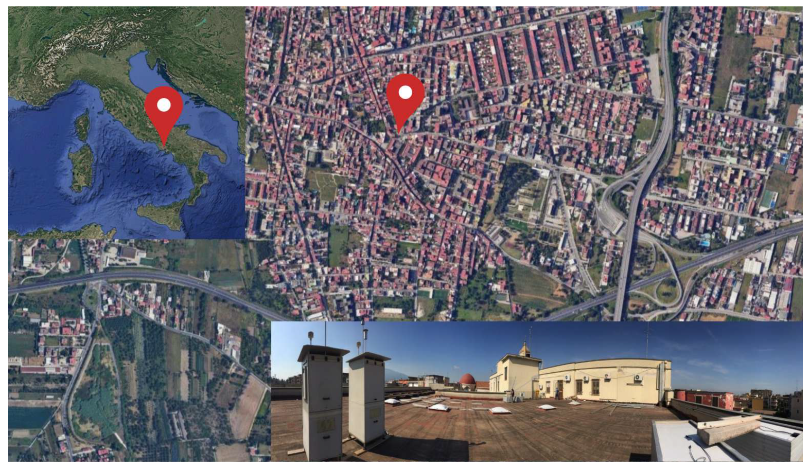
2.1. Atmospheric Measurements

The data for this study were collected within the MonAir Project, which focused on characterizing particulate matter in the urban environment of Pomigliano D’Arco, a highly urbanized and industrialized municipality east of Naples, Southern Italy (see Figure 1). Sampling and measurements were conducted on the rooftop of the City Hall building. Each sampling session lasted 24 h, with a daily air volume of 54.7 m3. Measurements spanned from January 2018 to December 2023. 24 h PM10 concentration determinations (midnight to midnight) were performed using a low-volume gravimetric sampler equipped with a 10 μm cut-off inlet. The instrument, a dual-channel beta attenuation monitor (SWAM5a Dual Channel Monitor, FAI Instruments, Fonte Nuova, Italy), operated at a flow rate of 2.3 m3/h. A 47 mm diameter quartz microfiber filter was used for collection. The instrument is TÜV- and CERT-certified as a beta monitor and complies with EU equivalence criteria for PM measurements, following EN 12341 and EN 14907 reference methods [22].

2.2. The Backward-Trajectory Method

In this work, ten-day (240 h) backward trajectories were determined through the numerical integration of trajectory equations. The calculation of backward air mass trajectories was conducted using the HYSPLIT 5.3.2 model (developed by the National Oceanic and Atmospheric Administration (NOAA) Air Resources Laboratory (ARL); https://www.ready.noaa.gov/HYSPLIT.php, (URL accessed on 15 February 2025), [1,23].
Air mass histories were based on the use of the 3-hourly meteorological data coming from NCEP’s GDAS (The National Center for Environmental Prediction, Global Data Assimilation System). NCEP collects meteorological data and performs computational analyses to generate weather forecasts four times daily. After analysis, data are converted from their initial spectral coefficient format into lat–long regular grids, at a 1.0 ° × 1.0 ° resolution, from sigma levels to mandatory pressure levels, and archived at the ARL. This process ensures that the data are formatted in a way that can be effectively used for predicting and understanding atmospheric conditions over time. Further information about this system is available on the ARL website (https://www.ready.noaa.gov/gdas1.php, URL accessed on 15 February 2025).
The backward trajectories started from the PdA monitoring site (40.907165° N, 14.392612° E), during the period from January 2018 to December 2023. Each air mass history was composed of an ensemble of 75 trajectories, with starting points uniformly distributed between 100 m and 1950 m above ground level at PdA. These trajectories were launched every six hours, resulting in four trajectory ensembles for each 24 h sampling period. At 5 min intervals along each trajectory, the three-dimensional position of the trajectory segment, temperature, humidity, and the height of the mixed layer were recorded.

2.3. Cluster Analysis

A cluster analysis was used to identify groups of airflow patterns that influenced the air quality at the PdA site. The HYSPLIT cluster analysis option was employed on the computed backward trajectories [24]. The clustering of trajectories was executed utilizing the total spatial variance (TSV) method, wherein clusters were aggregated through the minimization of the TSV, specifically the sum of all within-cluster variances.
The clustering process was initiated by assigning each trajectory to an individual ‘cluster’. Subsequently, the two clusters exhibiting the lowest increase in TSV were aggregated to form a pair, and the two clustered trajectories were replaced by their mean trajectory for further calculation. This process continued until the final merging of the last two clusters, resulting in the aggregation of all trajectories into a single cluster. The optimal number of clusters was ascertained by selecting the initial variation in the TSV between clusters that exceeded 30% within the last ten combinations. In this work, seven clusters were retained for the final analysis.
To determine the frequency of each air mass pattern over the analyzed period, and to avoid the potential for erroneous interpretations by assigning the same day to multiple airflow patterns, we exploited the concept of ‘core-days’ for identifying persistent airflow days [25]. Initially, the entire dataset underwent a classification procedure. Subsequently, if the majority of ensemble members corresponding to a particular day were categorized within the same cluster, the assignment was deemed robust, designating that day as a ‘core-day’. On the other hand, days failing to meet these criteria were omitted from further examination, as the assignment is highly sensitive to variability in transport patterns. A ‘core-day’ was characterized by a condition whereby at least 50% of the trajectories reaching PdA on a given day were assigned to the same cluster [26,27]. Application of this criterion revealed 1050 persistent days, accounting for 71% of the entire sampling period.

2.4. Residence Time Analysis

A residence time analysis (RT), originally introduced by [28,29], and subsequently refined by [30], was employed to quantify the duration air masses spent over specific regions prior to reaching the PdA site.
The RT method overlaid a grid on the region of interest and calculated the frequency and duration of trajectory endpoints within each grid cell. The result was a probability density function (pdf) that identified regions where air masses were more likely to accumulate or stagnate. The ridges of high probability in the pdf effectively delineated dominant pathways, enabling the inference of which regions were most influential in contributing to pollutant concentrations [28].
The derivation of the pdf governing the residence time analysis is provided in Appendix A. Let f ( r , θ ) denote the pdf of residence times at a distance r and direction θ from the receptor. Following [31], f ( r , θ ) was decomposed into ‘directional frequency’ and ‘potential accumulation’ components (see Equations (A3) and (A4)). The directional frequency represents the occurrence rate of transport between a source at ( r , θ ) and the receptor per unit arc length. Potential accumulation, defined as the inverse transport speed, indicates the average time air parcels reside over a unit radial length: the slower an air parcel moves over a region, the longer the time in which emissions in that region can accumulate in the air parcel.
The RT analysis was also used to assess variations in transport pathways with PM concentration. To this end, we computed the ratio
S ( r , θ ) = g ( r , θ ) f ( r , θ )
where g ( r , θ ) is the pdf of residence times for selected events, while f ( r , θ ) corresponds to all events. The ratio S ( r , θ ) identifies key source regions and transport dynamics contributing to pollution extremes. If S ( r , θ ) > 1 , residence times in the region ( r , θ ) exceed the expected average, suggesting a preferential transport pathway. Conversely, S ( r , θ ) < 1 indicates shorter residence times relative to the baseline.
We conducted a residence time analysis for trajectories associated with high and low PM10 concentrations, specifically when g ( r , θ ) corresponds to events above the 80th percentile and when it corresponds to events below the 20th percentile at the receptor site. This approach quantitatively assesses deviations in residence time distributions under specific conditions, offering insights into atmospheric transport mechanisms. Additionally, comparing S ( r , θ ) across regions provides a direct measure of their relative contributions to high/low concentrations at the receptor.

3. Results

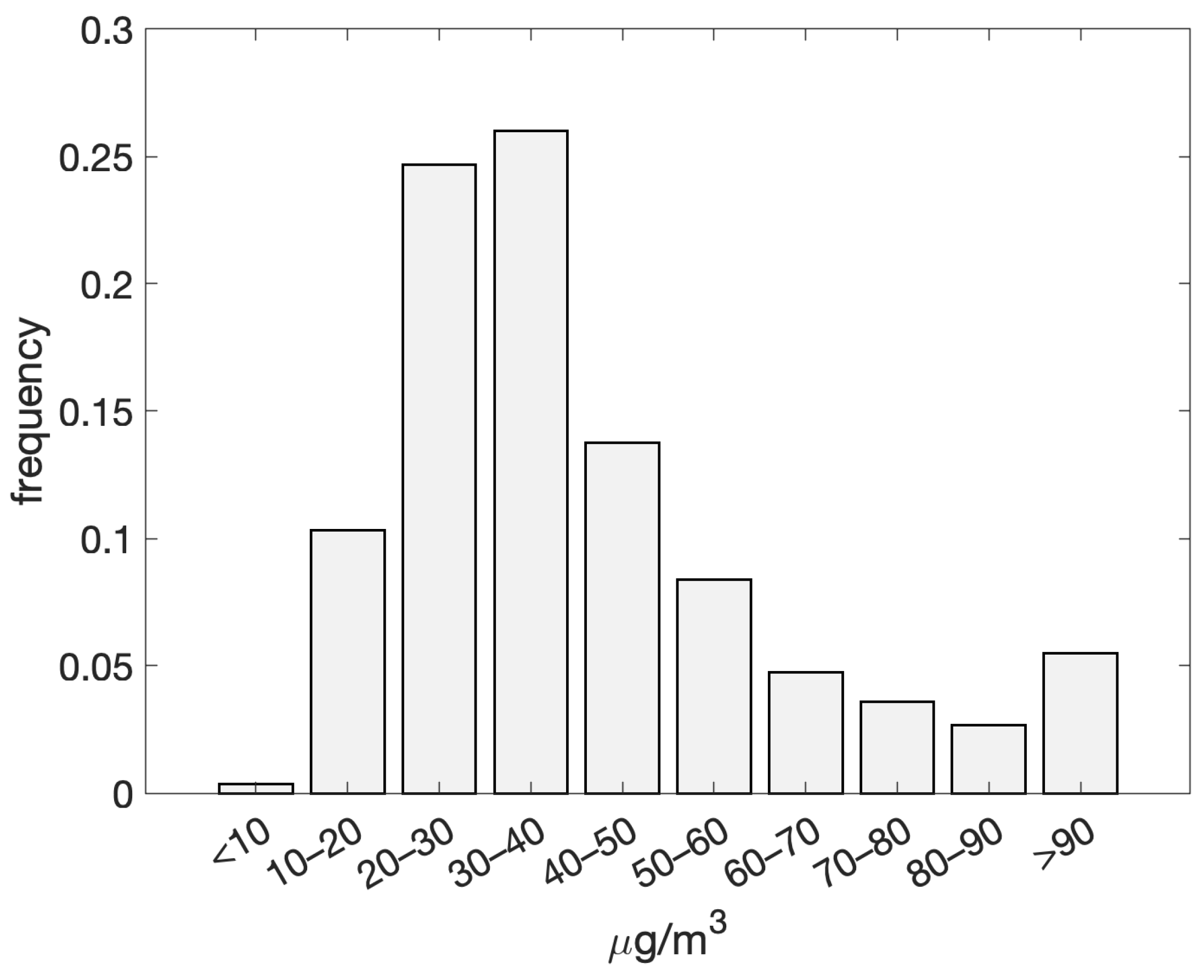
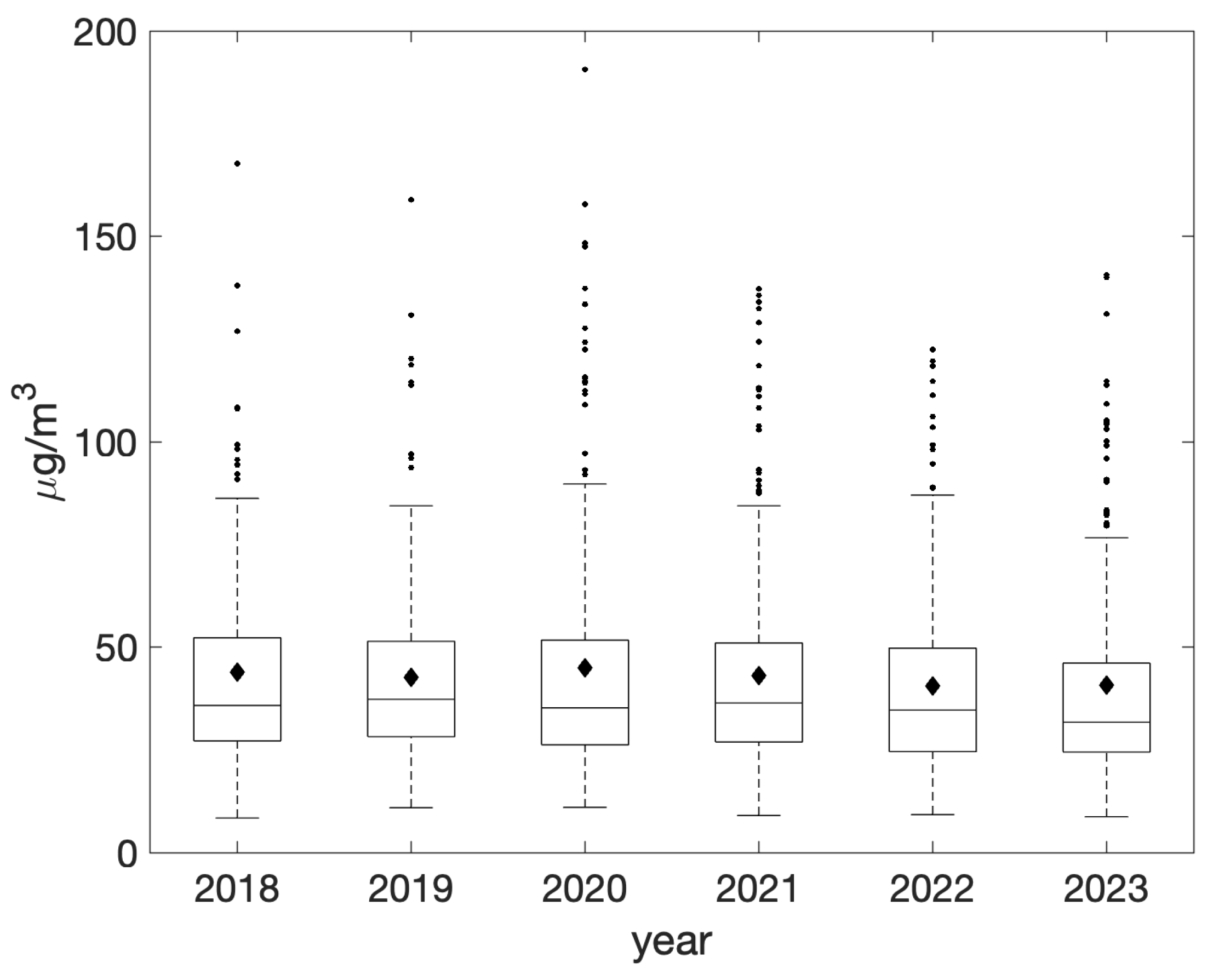
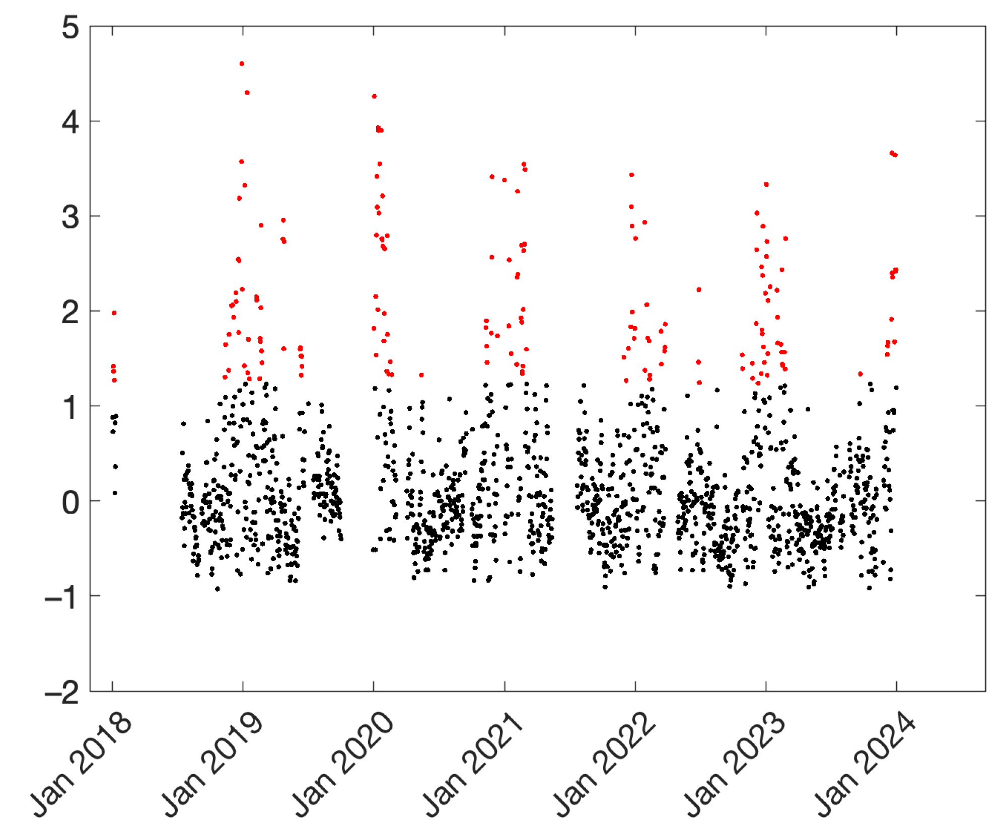
3.1. Descriptive Analysis of PM10 Concentrations

The distribution of daily PM10 concentrations recorded at the PdA monitoring site over the six-year period (2018–2023) is shown in Figure 2. The total number of valid data points amounted to 1620. Concentration levels displayed a pronounced peak within the 30–40 μg/m3 range, occurring in over 25% of cases, followed by the 20–30 μg/m3 range. As concentrations increased, the frequency exhibited a monotonic decline; nonetheless, a significant secondary peak was detected for occurrences exceeding 90 μg/m3, with over 5% of concentrations above this threshold.
Throughout the analyzed period, annual averages consistently exceeded the EU limit of 40 μg/m3, with a maximum of 44.9 μg/m3 recorded in 2020 (Figure 3). It is noteworthy that annual averages have demonstrated a consistent decrease, reaching a minimum value of 40.7 μg/m3 in 2023. Nevertheless, these concentrations persisted at levels considerably exceeding the annual average objective of 20 μg/m3 advocated by the new EU directive, which should be attained by 2030 [32].
The maximum and minimum number of days exceeding the EU daily threshold of 50 μg/m3—which should not be surpassed more than 35 times per year—occurred in 2019 and 2023, with 98 and 78 days, respectively.
The monthly average PM10 concentrations exhibited a pronounced peak during the winter months (December, January, and February; Figure 4), consistently exceeding the mean level of 55 μg/m3 across all three months. This trend was followed by a gradual decline, with the lowest concentrations recorded in May, and a slight increase during the summer months, probably due to the enhanced photochemical activity and secondary aerosol formation prompted by elevated temperatures and sunlight [33]. However, considerable monthly variability in the frequency of exceedance days was observed, with a notable concentration of anomalies during the winter months.

3.2. Comparison with Other Stations
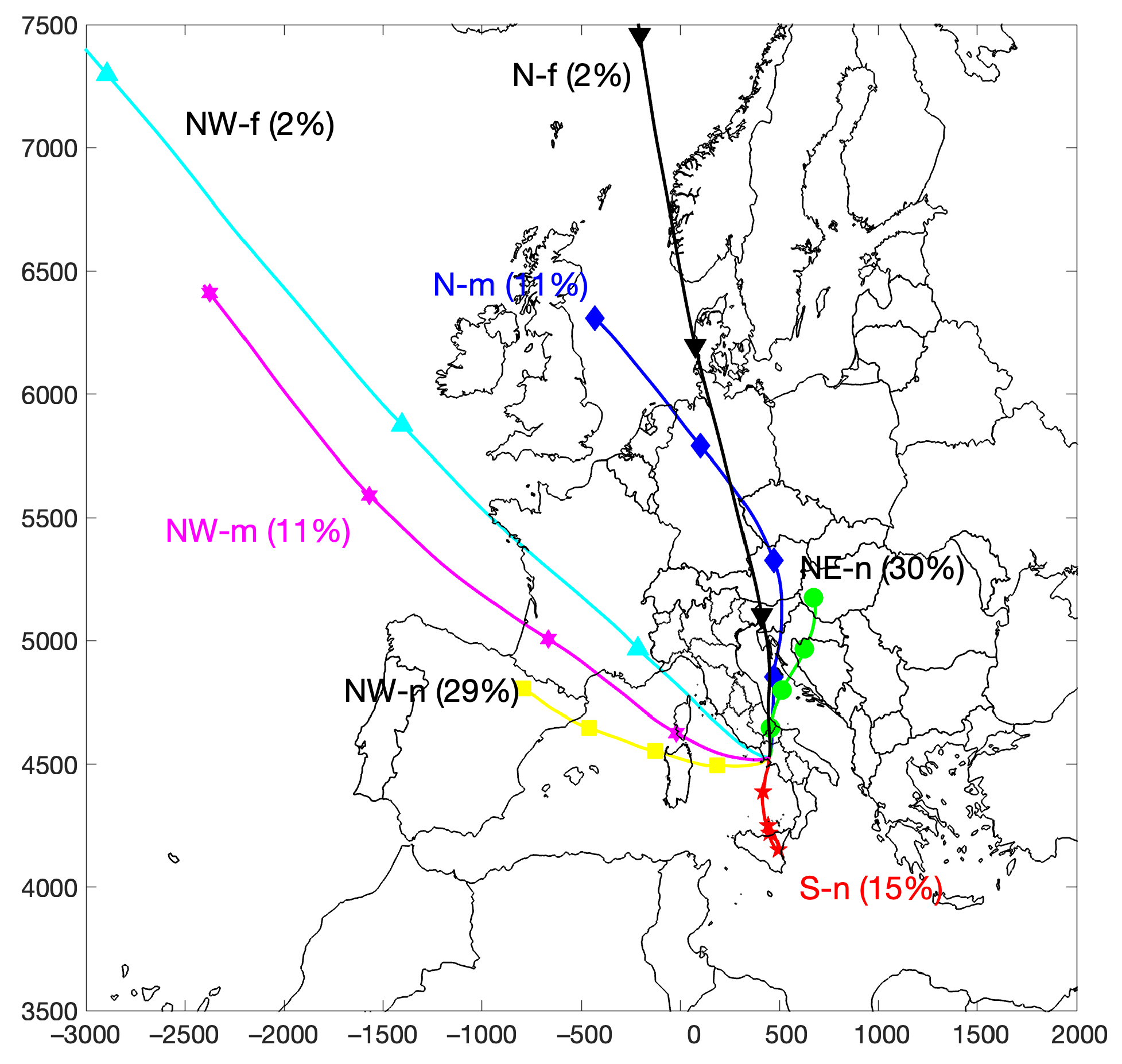
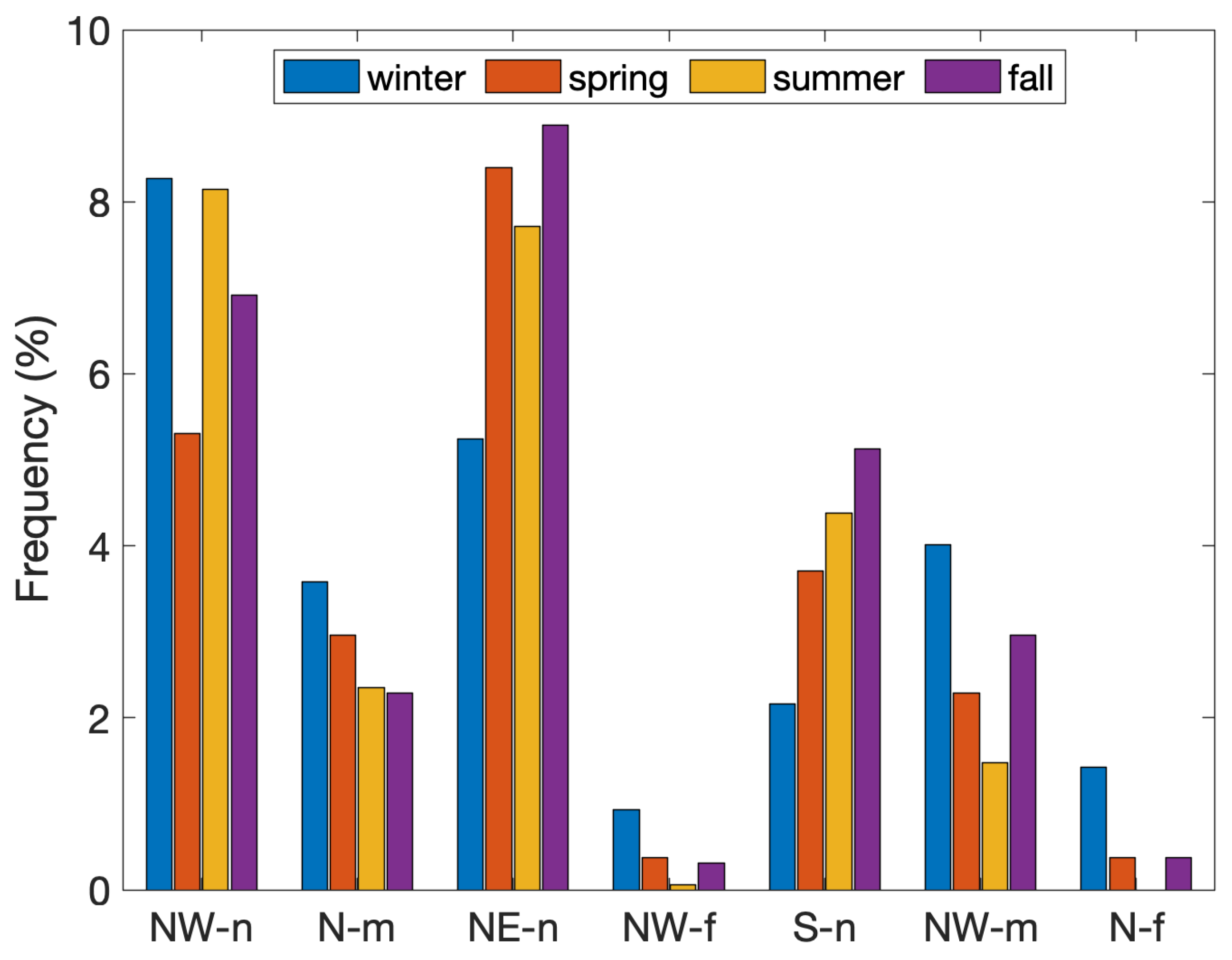
To assess the influence of meteorological conditions, we computed the correlations between PM10 concentrations measured at the PdA site and those of PM10 and PM2.5 recorded at nearby monitoring stations, all located within a maximum distance of 13 km from the PdA site. Data from these stations were obtained from the air quality monitoring database of the Campania region, accessible through the European Environment Agency website (https://eeadmz1-downloads-webapp.azurewebsites.net/, URL accessed on 15 February 2025). All selected stations are classified as either urban background or traffic monitoring sites within the metropolitan area of Naples.
The Pearson correlation coefficients between PdA and the other stations during the same sampling period are presented in Table 1. As observed, the correlation coefficients remained consistently high, with values not lower than 0.50 for PM10 and not lower than 0.47 for the correlation between PM10 at PdA and PM2.5 at the other stations. These relatively high values indicate that local emission sources are not the only contributing factor, highlighting the crucial role of large-scale meteorological conditions in homogenizing atmospheric PM concentrations.
The effects from large-scale meteorological conditions and the residence time analysis are reported in the following sections.
The importance of meteorological conditions can also be highlighted through the analysis of the results shown in Figure 5. This figure presents normalized PM10 data, i.e., data corrected according to the following expression:
c = C C ¯ σ C
where C ¯ represents the median value of the PM10 time series at the PdA site, and σ C is the corresponding standard deviation. Values greater than 1 indicate concentrations that exceed the median by at least one standard deviation.
The first notable observation is that the time series exhibits a clear right-skewed distribution, with low values not significantly below the mean, but with a number of positive anomalies considerably above the mean. The concentrations highlighted in red correspond to values exceeding the median by more than 1.5 times the interquartile range. According to this classification, 180 days were considered anomalous, specifically with a c-index above 1.236. These days were collectively indicated as ADs (anomalous days), and were usually associated with lower wind speed and higher-humidity conditions. The specific mean wind speed and relative humidity conditions are shown in Table 2. During ADs the wind speed is usually lower than during non-ADs, and the relative humidity is usually higher than during non-ADs, in accordance with previous studies [34,35,36],
Another interesting observation is that, among these 180 ADs, 23 were associated with dust conditions. Dust-affected days were defined as those showing evident transport from the south, as inferred from the analysis of backward trajectories. In cases of uncertainty, the analysis was complemented by the use of additional model outputs (e.g., CAMS—Copernicus Atmosphere Monitoring Service) or satellite data (i.e., TOMS/OMI UV Aerosol Index, MODIS AOD). During ADs the median PM10 concentration was 89.5 μg/m3, and for those associated with dust conditions, the median PM10 concentration was 93.1 μg/m3, highlighting the additional contribution of Saharan dust during anomalous days.

3.3. Airflow Paths

The cluster analysis of backward trajectories identified seven distinct airflow patterns influencing the PdA site, as depicted in Figure 6, showing their horizontal mean displacements throughout the stated period. The clusters were tagged according to their geographical origin and displacement relative to the source. Three clusters were characterized as northwesterly airflow, designated as NW-f (northwest—far), NW-m (northwest—medium), and NW-n (northwest—nearby); while three additional clusters originated from the north, identified as N-f (north—far), N-m (north—medium), and NE-n (northeast—nearby). Another cluster was associated with a southerly flow (S—nearby).
Figure 6 also displays the frequencies of occurrence for each cluster. The most frequent occurrences were for the NW-n and NE-n clusters, with frequencies of 29% and 30%, respectively. Infrequently, trajectories originated from the N-f and NW-f clusters, whereas the NW-m and N-m clusters showed intermediate frequencies of occurrence.
Figure 7 depicts the seasonal dynamics of airflow trajectories impacting PdA throughout the study period. This figure highlights the differences in the dynamic origin of air masses impacting the site, incorporating local circulation, short-range flows from the north and west, and sporadic long-range transport. These distinct airflow patterns exhibit pronounced seasonal variability. Local circulation emerged as the dominant feature of airflow patterns, exerting a consistent influence on PdA; this circulation accounted for a substantial proportion of airflows across all seasons, indicative of the influence of localized meteorological dynamics, such as topographical effects and thermal inversions, prevalent in regions with complex terrain, such as the area surrounding PdA. Specifically, nearby circulation from the north-east maintained a relatively stable influence throughout the seasons, contributing between 5 % of total trajectories in winter and 9 % in fall. This stability underscores the persistent nature of this circulation, likely associated with regional mesoscale weather patterns.
Airflows originating from the south exhibited a notable seasonal variation. During the winter months, southerly trajectories contributed minimally, averaging approximately 2 % . However, these flows increased in frequency during the summer and fall seasons, peaking at around 5 % , likely attributable to the heightened influence of convective processes and alterations in regional pressure gradients during warmer months. In contrast, northerly and northwesterly airflows exhibited a stronger influence during the winter, contributing on average 4 % of the total airflow. This seasonal predominance of northern air masses corresponds with the increased occurrence of cold front passages and high-pressure systems over central and southern Europe during winter, which often facilitates the advection of air masses from northern latitudes [37].

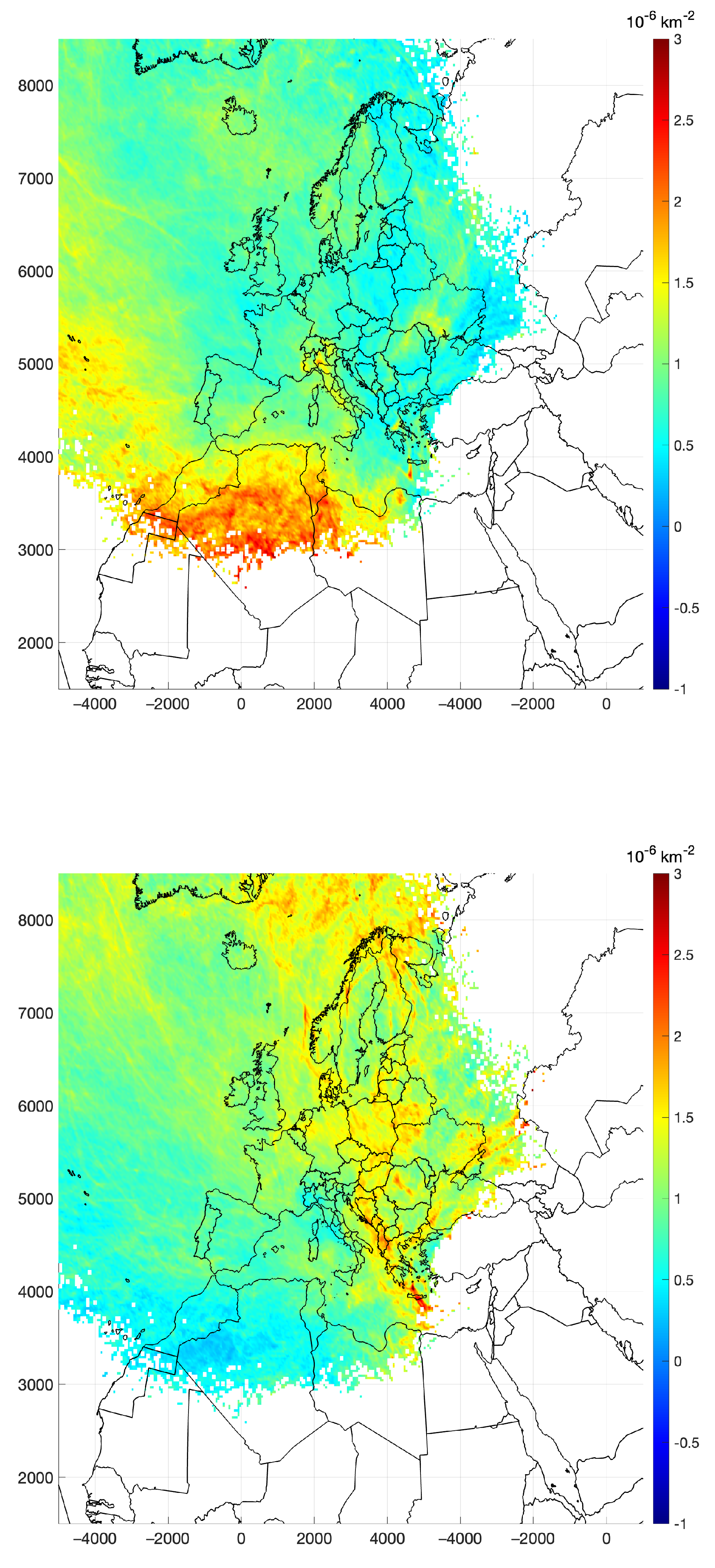
3.4. Residence Time Analysis

As described in Appendix A, a probability map was constructed and projected onto the Earth’s surface. To this end, trajectory endpoints were used to estimate the residence time (RT) probability map on a regular 25 × 25 km grid resolution (in UTM33 coordinates). To ensure the reliability of the analysis, uncertainties from the ensemble were addressed by the bootstrap method [38], by resampling the sample data (with replacement) among all trajectories belonging to the 75 members of each ensemble and performing inference about a sample from the resampled data. Retention of the p d f values for the residence time was conditioned on the cells with a mean value exceeding twice the estimated standard deviation.
The residence time calculation was conducted for three distinct sets of trajectories. A comprehensive residence time analysis was executed for the whole 6-year period. Subsequently, a second analysis focused on the subset of trajectories that reached PdA when PM10 concentrations exceeded the 80th percentile of the time series; and thirdly, a subset of trajectories when PM10 concentrations were below the 20th percentile. The RT pdfs derived from each of these analyses (and their decomposition into directional and accumulation potential; see Equation (A7)), provides insights into the geographical areas where air parcels influencing the receptor site most likely spent their time prior to the arrival at PdA during average-, high-, and low-pollution events.
Figure 8 represents the pdf for RT on a logarithmic color scale for the whole set of trajectories. As depicted, the predominant directions of arrival were from the northeasterly and westerly directions, corroborating the findings already found from cluster means in Figure 6, which reflected a similar pattern. This is consistent with a predominant influence at PdA of air masses originating from the northeastern part of Europe and from the western Mediterranean basin, usually associated with localized atmospheric circulation, including cyclonic or anti-cyclonic patterns and low wind conditions. The sharp gradient in residence times observed along geographical boundaries, such as the Alpine region, indicates the role of topography in modulating air mass transport pathways, potentially acting as a barrier to long-range advection, with little to no transport through this boundary. The impact of local topographical features is also evident. Figure 8 (upper-left panel) shows that the air masses that approach Naples mostly come from the eastern sector. This causes the channeling of sea/land breezes into the plain between the hills on the shoulders of the city and Mount Vesuvius. Lower residence times in areas such as northern Europe and southeastern regions of the Mediterranean basin contributed less frequently to the air composition at the receptor site during the analyzed period. The southeastern regions of the Mediterranean basin often exhibit nonsignificant values. Furthermore, the distribution underscores the influence of the central Mediterranean as a source or reservoir of atmospheric pollutants, with implications for air quality at this receptor site. High RT values in this region, due to the prevalence of nearby circulation patterns, point to stagnation events that enhance pollutant accumulation or recirculation.
The spatial patterns in the RT and transport directional frequency were quite similar (Figure 8). Therefore, the RT was predominantly due to the frequency at which trajectories traverse a given area prior to reaching the receptor. The distribution of accumulation potential exhibits considerable heterogeneity, with the most elevated values located within a band across the Italian peninsula, ranging from over 0.1 to 0.5 s/m, corresponding to effective air mass transport velocities of approximately 2 to 10 m/s. Notably, accumulation potentials were also observed over the Balkan region and the northern sector of the Saharan desert in areas identified by [39] as source regions in northern Africa.
Figure 9 provides the ratio of residence times during high- and low-pollution events. In particular, the ratio of the conditional probability (refer to Equation (1)) was computed for events during which the concentrations at the PdA site exceeded the 80th percentile or fell below the 20th percentile. Two prominent features are available from this figure: during high-pollution events, the regions contributing to emissions were located in the southeastern part of the domain, mainly from the Saharan region; nearby Italian regions, especially from Northern Italy and from the Tirrenian coast, also contribute to high pollution loads. Given that the residence time analysis pertains solely to the duration of the entire trajectory, the source–receptor analysis attributes a high conditional probability to segments traversing the Atlantic coasts. The maximum of the conditional probability east of the Canary Islands and the Morocco coastline was associated with trajectories passing first over the Atlantic Ocean and then northeastward over North Africa, where dust is actually mobilized, toward the Mediterranean basin, in agreement with [40]. Consequently, the observed maximum can be perceived as a potential artifact, attributing artificial emission sources to regions where several back trajectories associated with high-concentration events have traversed prior to reaching the actual source region.
During episodes of low pollution, atmospheric circulation was characterized by air mass trajectories originating from the northern European or northwestern Atlantic regions. As depicted in Figure 9, these trajectories from the northern sector were typically associated with low PM mass loading, which is likely due to their correlation with low emission levels and elevated wind velocities.
Upon delving deeper into the last statement, we specifically analyzed how PM10 concentrations depend on local meteorological conditions. To this end, Figure 10 shows the relationships between PM10 and meteorological variables (wind speed and relative humidity), for which we found a significant linear relationship (p-value < 0.05 ). These variables were extracted from the SYNOP messages of the Capodichino station, which is part of the monitoring network of the World Meteorological Organization (WMO), and is located near the sampling site (approximately 8 km away). The extracted data correspond to the daily average values of surface relative humidity and wind speed. The first panel depicts the influence of wind speed on PM10 concentrations. The observed negative correlation (p-value for the slope < 0.01) suggests that increasing wind speeds result in lower PM10 levels. The second panel displays the variation in PM10 concentrations as a function of relative humidity (RH%). The trend suggests a positive correlation (p-value for the slope < 0.002), indicating that higher RH levels are associated with increased PM10 concentrations.

4. Discussion

This study advances the understanding of particulate matter (PM10) transport dynamics in the Mediterranean region by integrating backward-trajectory analysis, cluster analysis, and residence time analysis to investigate air mass pathways and their contributions to PM10 concentrations at the PdA site, offering insights into the interplay of local emissions, regional transport mechanisms, and meteorological conditions. While earlier research has predominantly examined remote or rural locations in the Mediterranean basin [3,15], this work highlights the compound effects of local emissions and regional transport in a densely populated and industrialized region.
The analysis of PM10 concentrations during the period 2018–2023 clearly shows the high PM loads at this receptor. The distinctive characteristics of this site are evident in the distribution of daily data, which predominantly show values concentrated in the range of 20–40 μg/m3, and a slow and gradual decline in the frequency at higher concentration levels, accompanied by occurrences of extreme values exceeding 90 μg/m3. When compared to other urban and industrialized regions, PM10 levels at PdA are notably high. For instance, annual averages at PdA exceed those reported for similarly industrialized areas such as Milan and Turin in Northern Italy, where averages range between 30 and 40 μg/m3 [41]. In Mediterranean urban centers such as Barcelona and Athens, PM10 levels are typically lower, averaging around 25–35 μg/m3, reflecting differences in local emission sources and regional meteorological influences [42]. These findings highlight the unique challenges posed by the combination of local emissions, complex topographical features, and transboundary pollutant transport at the PdA site in Southern Italy.
Variations in daily values throughout the year are indicative of seasonal fluctuations in emission sources and synoptic/local meteorological conditions (e.g., [41]). The monthly variations in PM10 concentrations exhibit a pronounced increase during the colder months. This phenomenon at the PdA station can be ascribed to a heightened dependence on residential heating, coupled with reduced atmospheric dispersion due to temperature inversions, which confine pollutants near the surface level [43,44]. Furthermore, the increase in concentrations observed during the summer can likely be attributed to enhanced photochemical activity and the formation of secondary aerosols driven by elevated temperatures and sunlight, thereby exacerbating urban pollution [33].
The identification of seven distinct airflow patterns exemplifies the interplay of synoptic-scale meteorological conditions influencing the region. These patterns are governed by synoptic phenomena, notably including the extended subtropical anticyclone of the Atlantic (Azores) and the North Atlantic Oscillation [15,45,46,47]. Predominantly, local circulation prevails throughout the year, primarily originating from the northeastern and western directions. Although less frequent, southerly circulation denotes the impact of cyclonic activity within the Mediterranean and the advection of air masses from North Africa [48]. More specifically, during spring, large amounts of mineral particles are transported, mainly from the Sahara desert, towards the Mediterranean and Europe [14]. The transport is facilitated by the prevailing south-southwesterly winds induced by depressions advancing eastwards along the North African coast. In the summer months, the transport of Saharan dust within the western and central Mediterranean basin occurs because of thermal lows situated either over northwestern Africa or the Iberian Peninsula [14,49]. In contrast, the highest frequencies of the fast northerly and westerly patterns occur in winter, associated with stronger pressure gradients and enhanced zonal flow typical of the winter season, leading to rapid transport of air masses from distant regions [50].
The interaction between local topographical features and the proximity to the Mediterranean sea leads to the formation of nearby circulation patterns, influenced by thermal contrasts, thereby increasing the complexity of airflow in this region. Elevated PM10 concentrations are observed under these regional circulation patterns, particularly from the NE-n and NW-n directions. These results align with prior research indicating that regional circulation patterns exert a considerable influence on air quality in urban areas across the Mediterranean [51]. This influence is further corroborated by the frequency analysis of exceedance days, where PM10 concentrations exceed the EU’s daily limit of 50 μg/m3. Specifically, these nearby circulation patterns are responsible for 75% of the days with elevated pollution levels, highlighting the role of slow-moving air masses originating near Naples in facilitating pollutant accumulation [52].
The temporal and spatial distribution of residence times play a pivotal role in shaping the transport of pollutants and their potential accumulation in the region. The highest residence times are observed in proximity to the central Mediterranean area, indicating dominant local circulations. This finding highlights the importance of local sources in contributing to the regional air quality. Furthermore, elevated residence times are present along pathways extending to northern Africa and southeastern Europe, suggesting that long-range transport mechanisms also play a significant role during specific periods. The influence of the Sahara, particularly during dust episodes, aligns with prior studies demonstrating its impact on particulate matter concentrations in the Mediterranean basin [42,53].
Seasonal differences in the backward trajectories emphasize the interplay between meteorological conditions and pollutant transport. During the summer months, air masses originating from northern Africa were more prevalent, consistent with the enhanced desert dust transport typical of this season. In contrast, the winter period exhibited a higher frequency of trajectories from Europe, reflecting the influence of continental sources and synoptic-scale weather patterns. These results corroborate findings from similar studies conducted in the Mediterranean region [16,17]. The analysis also revealed that residence times are inversely related to the transport speed of air masses. Regions with higher residence times correspond to slower-moving air masses, allowing for greater accumulation of pollutants. This observation underscores the role of stagnant atmospheric conditions in exacerbating air quality issues. Areas with shorter residence times, typically associated with faster-moving air masses, exhibited lower pollutant concentrations, indicating efficient dispersion and dilution mechanisms. In terms of air quality, the residence time patterns imply that emissions from anthropogenic or natural sources within the highlighted high-RT regions are likely to have a significant impact on pollutant levels at the receptor site.
Finally, Figure 10 depicts correlations between PM levels and various meteorological variables throughout the sampling period, revealing several noteworthy trends. During days with higher wind speeds, PM concentrations tend to decrease. This observation aligns with established research demonstrating that wind facilitates the dispersion of airborne pollutants, thereby improving air quality. For instance, Garrido-Perez et al. [54] examined air stagnation events in Europe, highlighting that light winds contribute to the accumulation of pollutants, whereas stronger winds aid in their dispersal. Similar results have been reported for the US [55], China [56], and India [57]. However, it is also important to consider that very high wind speeds may contribute to the resuspension of dust and sea salt aerosols, potentially leading to localized increases in PM10 under certain conditions. This is evident from the right tail of the bar histogram in Figure 10, where higher wind speeds do not cause a clear and progressive decrease in concentration.
At the same time, this figure also shows that increased relative humidity conditions promote the accumulation and formation of particulate matter. This could be attributed to multiple factors. First, hygroscopic growth of aerosol particles can lead to an increase in their mass, thereby elevating PM10 concentrations. Additionally, high-RH conditions often correspond to stable atmospheric conditions, which limit dispersion and promote pollutant accumulation. Another contributing factor could be the enhanced secondary aerosol formation under high humidity, further augmenting PM concentrations. Notably, the highest PM10 concentrations occur when RH exceeds 90%, reinforcing the role of moisture in particle growth and accumulation [58].

5. Conclusions

This backward-trajectory analysis provides a comprehensive understanding of the atmospheric transport processes affecting the PdA site in a central Mediterranean region. Local circulation and long-range transport from northern Africa and Europe are the primary contributors to the observed air quality patterns. Seasonal variations in trajectory origins reflect the dynamic nature of atmospheric circulation and its implications for pollutant transport.
The implications of this study are significant for air quality management in the Mediterranean region. The identification of the central Mediterranean and northern Africa as key contributors to high PM10 levels underscores the need for transboundary policies that address both local emissions and regional transport. Furthermore, the findings emphasize the importance of targeted interventions during periods of stagnation, such as reducing emissions from industrial and residential heating sources in winter. These results complement the observations of Putaud et al. [41], who highlighted the need for localized emission control measures, by providing specific evidence from an urban–industrial context, i.e., by emphasizing both local and transboundary actions to mitigate particulate matter pollution. In the case of the PdA site, long-term strategies should integrate urban planning and sustainable development practices to mitigate PM10 pollution, balancing approaches that combine regulatory enforcement, technological innovation, public awareness, and transboundary collaboration. Such strategies not only address the immediate challenge of PM10 pollution but also contribute to the broader goals of environmental sustainability and public health protection.
Finally, this study opens new avenues for future research. The integration of residence time analysis with chemical transport models, such as WRF-Chem or CAMx, could enhance source apportionment by quantifying the relative contributions of natural and anthropogenic sources. Additionally, the potential impacts of climate change on atmospheric circulation patterns and pollutant transport warrant further investigation, as shifting synoptic conditions may alter the dynamics of PM10 accumulation in the Mediterranean basin.

Author Contributions

Conceptualization, A.R. and M.T. (Marco Trifuoggi); methodology, A.R. and M.T. (Marco Trifuoggi); validation, A.R. and E.C.; formal analysis, A.R.; investigation, A.G., M.A. and M.T. (Maria Toscanesi); resources, A.R., M.A. and M.T. (Marco Trifuoggi); data curation, A.R., E.C., A.G. and M.T. (Maria Toscanesi); writing—original draft preparation, A.G., A.R., E.C., M.A., M.T. (Maria Toscanesi) and M.T. (Marco Trifuoggi); writing—review and editing, A.R.; funding acquisition, M.T. (Marco Trifuoggi). All authors have read and agreed to the published version of the manuscript.

Funding

This research was funded by the Municipality of Pomigliano d’Arco, under the MONAIR project.

Institutional Review Board Statement

Not applicable.

Informed Consent Statement

Not applicable.

Data Availability Statement

Data and software analysis may be available from authors on request.

Acknowledgments

The authors acknowledge the Municipality of Pomigliano D’Arco (NA) for supporting the MONAIR project.

Conflicts of Interest

The authors declare no conflicts of interest.

Appendix A. The Probability Density Function Associated with Residence Time

The two-dimensional residence time (RT) depends on how frequently air mass trajectories pass over a grid cell and the time they remain within it. As outlined in [28,31], in the case of straight trajectories moving at constant speed, u, and duration, τ , the probability density function for RT in polar coordinates, ( θ , r ), assumes the following form:
f ( θ , r ) = H ( θ ) 2 π r u τ
where H ( θ ) indicates the density of trajectories from direction θ . The expression takes the form
H ( θ ) = h ( θ ) h ¯
where h ¯ denotes the mean density of trajectories spanning from 0 to 2 π , and h ( θ ) represents the density per unit radiant. u τ R max is the maximum distance traveled, on the assumption of a rectilinear trajectory and constant speed.
f can be conceptualized as comprising two distinct components: the transport directional frequency and the accumulation potential. The transport directional frequency quantifies the likelihood of air mass transport occurring between a source and receptor per unit arc length, equivalent to
D = H ( θ ) 2 π r
which decreases with distance due to the spread of trajectories over a larger area. The accumulation potential quantifies the time air parcels spend over a specific region, and is inversely related to transport speed:
A P = 1 u
This measure encapsulates the extent to which emissions originating from a specific region contribute to the accumulation of pollutants in air parcels. Indeed, as the velocity of an air parcel’s movement over a region decreases, the duration during which emissions from that region accumulate within the air parcel increases. Given these two definitions, f can be expressed as
f ( r , θ ) = D × A P τ
In its discrete form, D ( r , θ ) is averaged over the arc length of each grid cell, and the resulting value quantifies the frequency of trajectory crossings relative to the grid cell area.
D i , j = 1 L 1 T t = 1 T t r i , j , t
where D i , j has units of m−1; index i runs over all trajectories whose number is T; t r i , j , t is unit if trajectory t traverses grid cell ( i , j ) , and 0 otherwise; and L is a length scale, where L 2 is the area of the grid cell. Similarly, the discrete accumulation potential is derived as the mean time trajectories reside within a cell, normalized by the grid cell’s radial length:
A P i , j = n ¯ i , j Δ τ L ,
where
n ¯ i , j = 1 t = 1 T t r i , j , t t = 1 T n i , j , t
where A P i , j   [ s   m 1 ] is the discrete accumulation potential for grid cell ( i , j ) ; n i , j , t is the number of trajectory segment endpoints in grid cell ( i , j ) for trajectory t; n ¯ i , j is the average number of trajectory segment endpoints per trajectory in the grid cell ( i , j ) ; and Δ τ   [ s ] is the time interval between each trajectory segment endpoint.
These parameters are combined to estimate the pdf for the residence time in grid cell ( i , j ) as
f ( i , j ) = D i . j A P i , j / τ

References

  1. Stein, A.F.; Draxler, R.R.; Rolph, G.D.; Stunder, B.J.; Cohen, M.D.; Ngan, F. NOAA’s HYSPLIT atmospheric transport and dispersion modeling system. Bull. Am. Meteorol. Soc. 2015, 96, 2059–2077. [Google Scholar]
  2. Bakels, L.; Tatsii, D.; Tipka, A.; Thompson, R.; Dütsch, M.; Blaschek, M.; Seibert, P.; Baier, K.; Bucci, S.; Cassiani, M.; et al. FLEXPART version 11: Improved accuracy, efficiency, and flexibility. Geosci. Model Dev. 2024, 17, 7595–7627. [Google Scholar]
  3. Kahl, J.D.; Martinez, D.A.; Kuhns, H.; Davidson, C.I.; Jaffrezo, J.L.; Harris, J.M. Air mass trajectories to Summit, Greenland: A 44-year climatology and some episodic events. J. Geophys. Res. 1997, 102, 26861–26875. [Google Scholar]
  4. Tositti, L.; Riccio, A.; Sandrini, S.; Brattich, E.; Baldacci, D.; Parmeggiani, S.; Cristofanelli, P.; Bonasoni, P. Short-term climatology of PM10 at a high altitude background station in southern Europe. Atmos. Environ. 2013, 65, 142–152. [Google Scholar]
  5. Liao, H.; Wu, C. Investigation of source locations and contributions using an integrated trajectory-source apportionment method with multiple time resolution data. Int. J. Environ. Sci. Technol. 2017, 14, 1781–1786. [Google Scholar] [CrossRef]
  6. Hsu, Y.K.; Holsen, T.M.; Hopke, P.K. Comparison of hybrid receptor models to locate PCB sources in Chicago. Atmos. Environ. 2003, 37, 545–562. [Google Scholar]
  7. Reimann, S.; Schaub, D.; Stemmler, K.; Folini, D.; Hill, M.; Hofer, P.; Buchmann, B.; Simmonds, P.G.; Greally, B.R.; O’Doherty, S. Halogenated greenhouse gases at the Swiss High Alpine Site of Jungfraujoch (3580 m asl): Continuous measurements and their use for regional European source allocation. J. Geophys. Res. Atmos. 2004, 109. [Google Scholar]
  8. Wang, L.; Lyu, B.; Bai, Y. Aerosol vertical profile variations with seasons, air mass movements and local PM2.5 levels in three large China cities. Atmos. Environ. 2020, 224, 117329. [Google Scholar]
  9. Merico, E.; Cesari, D.; Gregoris, E.; Gambaro, A.; Cordella, M.; Contini, D. Shipping and air quality in Italian port cities: State-of-the-art analysis of available results of estimated impacts. Atmosphere 2021, 12, 536. [Google Scholar] [CrossRef]
  10. Chianese, E.; Tirimberio, G.; Appolloni, L.; Dinoi, A.; Contini, D.; Di Gilio, A.; Palmisani, J.; Cotugno, P.; Miniero, D.V.; Dusek, U.; et al. Chemical characterisation of PM10 from ship emissions: A study on samples from hydrofoil exhaust stacks. Environ. Sci. Pollut. Res. 2022, 29, 17723–17736. [Google Scholar]
  11. Pietrodangelo, A.; Bove, M.C.; Forello, A.C.; Crova, F.; Bigi, A.; Brattich, E.; Riccio, A.; Becagli, S.; Bertinetti, S.; Calzolai, G.; et al. A PM10 chemically characterized nation-wide dataset for Italy. Geographical influence on urban air pollution and source apportionment. Sci. Total Environ. 2024, 908, 167891. [Google Scholar] [PubMed]
  12. EEA. Europe’s Air Quality Status 2024; Technical Report; European Environment Agency: Copenhagen, Denmark, 2024. [Google Scholar]
  13. WHO. Air Quality, Energy, and Health; Technical Report; World Health Organization: Geneva, Switzerland, 2021. [Google Scholar]
  14. Barnaba, F.; Gobbi, G. Aerosol seasonal variability over the Mediterranean region and relative impact of maritime, continental and Saharan dust particles over the basin from MODIS data in the year 2001. Atmos. Chem. Phys. 2004, 4, 2367–2391. [Google Scholar] [CrossRef]
  15. Gkikas, A.; Houssos, E.; Hatzianastassiou, N.; Papadimas, C.; Bartzokas, A. Synoptic conditions favouring the occurrence of aerosol episodes over the broader Mediterranean basin. Q. J. R. Meteorol. Soc. 2012, 138, 932–949. [Google Scholar] [CrossRef]
  16. Querol, X.; Tobías, A.; Pérez, N.; Karanasiou, A.; Amato, F.; Stafoggia, M.; García-Pando, C.P.; Ginoux, P.; Forastiere, F.; Gumy, S.; et al. Monitoring the impact of desert dust outbreaks for air quality for health studies. Environ. Int. 2019, 130, 104867. [Google Scholar]
  17. Rodrıguez, S.; Querol, X.; Alastuey, A.; Kallos, G.; Kakaliagou, O. Saharan dust contributions to PM10 and TSP levels in Southern and Eastern Spain. Atmos. Environ. 2001, 35, 2433–2447. [Google Scholar]
  18. Koo, J.H.; Lee, D.; Bae, H.; Lee, T.; Na, S.G.; Yeh, S.W.; Park, J.; Yeo, M. Back-trajectory analyses for evaluating the transboundary transport effect to the aerosol pollution in South Korea. Environ. Pollut. 2024, 351, 124031. [Google Scholar]
  19. Poddubny, V.; Nagovitsyna, E.; Antonov, K.; Markelov, J.; Buevich, A.; Omelkova, E.; Manzhurov, I.; Medvedev, A.; Vasilyeva, J. Estimation of the atmospheric greenhouse gas spatial distribution in the Arctic using a back trajectory model. Math. Methods Appl. Sci. 2020, 43, 7657–7663. [Google Scholar]
  20. Jain, C.D.; Singh, V.; Raj, S.A.; Madhavan, B.; Ratnam, M.V. Local emission and long-range transport impacts on the CO, CO2, and CH4 concentrations at a tropical rural site. Atmos. Environ. 2021, 254, 118397. [Google Scholar]
  21. Li, C.; Dai, Z.; Liu, X.; Wu, P. Transport Pathways and Potential Source Region Contributions of PM2.5 in Weifang: Seasonal Variations. Appl. Sci. 2020, 10, 2835. [Google Scholar] [CrossRef]
  22. Perrino, C.; Giusto, M.; Sargolini, T.; Calzolai, G.; Canepari, S. Assessment of the link between atmospheric dispersion and chemical composition of PM10 at 2-h time resolution. Chemosphere 2022, 298, 134272. [Google Scholar]
  23. Draxler, R. HYSPLIT4 User’s Guide NOAA Tech; Technical Report; Memo. ERL ARL-230; NOAA Air Resources Laboratory: Silver Spring, MD, USA, 1999. [Google Scholar]
  24. Draxler, R.; Stunder, B.; Rolph, G.; Stein, A.; Taylor, A. HYSPLIT Tutorial. 2023. Available online: https://www.ready.noaa.gov/documents/Tutorial/html/index.html (accessed on 15 February 2025).
  25. Cape, J.; Methven, J.; Hudson, L. The use of trajectory cluster analysis to interpret trace gas measurements at Mace Head, Ireland. Atmos. Environ. 2000, 34, 3651–3663. [Google Scholar]
  26. Riccio, A.; Giunta, G.; Chianese, E. The application of a trajectory classification procedure to interpret air pollution measurements in the urban area of Naples (Southern Italy). Sci. Total Environ. 2007, 376, 198–214. [Google Scholar] [CrossRef]
  27. Riccio, A.; Chianese, E.; Agrillo, G.; Esposito, C.; Ferrara, L.; Tirimberio, G. Source apportion of atmospheric particulate matter: A joint Eulerian/Lagrangian approach. Environ. Sci. Pollut. Res. 2014, 21, 13160–13168. [Google Scholar]
  28. Ashbaugh, L.L.; Malm, W.C.; Sadeh, W.Z. A residence time probability analysis of sulfur concentrations at Grand Canyon National Park. Atmos. Environ. 1985, 19, 1263–1270. [Google Scholar]
  29. Poirot, R.L.; Wishinski, P.R. Visibility, sulfate and air mass history associated with the summertime aerosol in northern Vermont. Atmos. Environ. 1986, 20, 1457–1469. [Google Scholar] [CrossRef]
  30. Stohl, A. Computation, accuracy and applications of trajectories—A review and bibliography. Atmos. Environ. 1998, 32, 947–966. [Google Scholar]
  31. Schichtel, B.A.; Gebhart, K.A.; Barna, M.G.; Malm, W.C. Association of airmass transport patterns and particulate sulfur concentrations at Big Bend National Park, Texas. Atmos. Environ. 2006, 40, 992–1006. [Google Scholar]
  32. Council of European Union. Directive 2024/2881 of the European Parliament and of the Council of 23 October 2024 on Ambient Air Quality and Cleaner Air for Europe; Council of European Union: Brussels, Belgium, 2024. [Google Scholar]
  33. Zhang, R.; Wang, G.; Guo, S.; Zamora, M.L.; Ying, Q.; Lin, Y.; Wang, W.; Hu, M.; Wang, Y. Formation of urban fine particulate matter. Chem. Rev. 2015, 115, 3803–3855. [Google Scholar] [CrossRef]
  34. Liu, X.; Chang, M.; Zhang, J.; Wang, J.; Gao, H.; Gao, Y.; Yao, X. Rethinking the causes of extreme heavy winter PM2.5 pollution events in northern China. Sci. Total Environ. 2021, 794, 148637. [Google Scholar]
  35. Shikhovtsev, M.Y.; Molozhnikova, Y.V.; Obolkin, V.A.; Potemkin, V.L.; Lutskin, E.S.; Khodzher, T.V. Features of Temporal Variability of the Concentrations of Gaseous Trace Pollutants in the Air of the Urban and Rural Areas in the Southern Baikal Region (East Siberia, Russia). Appl. Sci. 2024, 14, 8327. [Google Scholar] [CrossRef]
  36. Baltaci, H.; Arslan, H.; Akkoyunlu, B. High PM10 source regions and their influence on respiratory diseases in Canakkale, Turkey. Int. J. Environ. Sci. Technol. 2022, 19, 797–806. [Google Scholar] [CrossRef]
  37. Rüdisühli, S.; Sprenger, M.; Leutwyler, D.; Schär, C.; Wernli, H. Attribution of precipitation to cyclones and fronts over Europe in a kilometer-scale regional climate simulation. Weather Clim. Dyn. 2020, 1, 675–699. [Google Scholar]
  38. Tibshirani, R.J.; Efron, B. An Introduction to the Bootstrap; Monographs on Statistics and Applied Probability, Volume 57; Chapman and Hall, Inc.: Boca Raton, FL, USA, 1993; pp. 1–436. [Google Scholar]
  39. Prospero, J.M.; Ginoux, P.; Torres, O.; Nicholson, S.E.; Gill, T.E. Environmental characterization of global sources of atmospheric soil dust identified with the Nimbus 7 Total Ozone Mapping Spectrometer (TOMS) absorbing aerosol product. Rev. Geophys. 2002, 40, 2-1–2-31. [Google Scholar]
  40. Israelevich, P.; Ganor, E.; Alpert, P.; Kishcha, P.; Stupp, A. Predominant transport paths of Saharan dust over the Mediterranean Sea to Europe. J. Geophys. Res. Atmos. 2012, 117, D02205. [Google Scholar]
  41. Putaud, J.P.; Van Dingenen, R.; Alastuey, A.; Bauer, H.; Birmili, W.; Cyrys, J.; Flentje, H.; Fuzzi, S.; Gehrig, R.; Hansson, H.C.; et al. A European aerosol phenomenology–3: Physical and chemical characteristics of particulate matter from 60 rural, urban, and kerbside sites across Europe. Atmos. Environ. 2010, 44, 1308–1320. [Google Scholar] [CrossRef]
  42. Querol, X.; Pey, J.; Pandolfi, M.; Alastuey, A.; Cusack, M.; Pérez, N.; Moreno, T.; Viana, M.; Mihalopoulos, N.; Kallos, G.; et al. African dust contributions to mean ambient PM10 mass-levels across the Mediterranean Basin. Atmos. Environ. 2009, 43, 4266–4277. [Google Scholar]
  43. Janhäll, S.; Olofson, K.F.G.; Andersson, P.U.; Pettersson, J.B.; Hallquist, M. Evolution of the urban aerosol during winter temperature inversion episodes. Atmos. Environ. 2006, 40, 5355–5366. [Google Scholar]
  44. Li, Z.; Guo, J.; Ding, A.; Liao, H.; Liu, J.; Sun, Y.; Wang, T.; Xue, H.; Zhang, H.; Zhu, B. Aerosol and boundary-layer interactions and impact on air quality. Natl. Sci. Rev. 2017, 4, 810–833. [Google Scholar] [CrossRef]
  45. Xoplaki, E.; González-Rouco, J.F.; Luterbacher, J.; Wanner, H. Mediterranean summer air temperature variability and its connection to the large-scale atmospheric circulation and SSTs. Clim. Dyn. 2003, 20, 723–739. [Google Scholar]
  46. Xoplaki, E.; González-Rouco, J.; Luterbacher, J.; Wanner, H. Wet season Mediterranean precipitation variability: Influence of large-scale dynamics and trends. Clim. Dyn. 2004, 23, 63–78. [Google Scholar]
  47. Krichak, S.; Alpert, P. Signatures of the NAO in the atmospheric circulation during wet winter months over the Mediterranean region. Theor. Appl. Climatol. 2005, 82, 27–39. [Google Scholar]
  48. Michaelides, S.; Karacostas, T.; Sánchez, J.L.; Retalis, A.; Pytharoulis, I.; Homar, V.; Romero, R.; Zanis, P.; Giannakopoulos, C.; Bühl, J.; et al. Reviews and perspectives of high impact atmospheric processes in the Mediterranean. Atmos. Res. 2018, 208, 4–44. [Google Scholar]
  49. Papadimas, C.; Hatzianastassiou, N.; Mihalopoulos, N.; Querol, X.; Vardavas, I. Spatial and temporal variability in aerosol properties over the Mediterranean basin based on 6-year (2000–2006) MODIS data. J. Geophys. Res. Atmos. 2008, 113. [Google Scholar] [CrossRef]
  50. Trigo, I.F.; Bigg, G.R.; Davies, T.D. Climatology of cyclogenesis mechanisms in the Mediterranean. Mon. Weather Rev. 2002, 130, 549–569. [Google Scholar] [CrossRef]
  51. Querol, X.; Alastuey, A.; Moreno, T.; Viana, M.; Castillo, S.; Pey, J.; Rodríguez, S.; Artiñano, B.; Salvador, P.; Sánchez, M.; et al. Spatial and temporal variations in airborne particulate matter (PM10 and PM2.5) across Spain 1999–2005. Atmos. Environ. 2008, 42, 3964–3979. [Google Scholar] [CrossRef]
  52. Kallos, G.; Kotroni, V.; Lagouvardos, K.; Papadopoulos, A. On the long-range transport of air pollutants from Europe to Africa. Geophys. Res. Lett. 1998, 25, 619–622. [Google Scholar] [CrossRef]
  53. Gkikas, A.; Hatzianastassiou, N.; Mihalopoulos, N.; Katsoulis, V.; Kazadzis, S.; Pey, J.; Querol, X.; Torres, O. The regime of intense desert dust episodes in the Mediterranean based on contemporary satellite observations and ground measurements. Atmos. Chem. Phys. 2013, 13, 12135–12154. [Google Scholar]
  54. Garrido-Perez, J.M.; Ordóñez, C.; García-Herrera, R.; Barriopedro, D. Air stagnation in Europe: Spatiotemporal variability and impact on air quality. Sci. Total Environ. 2018, 645, 1238–1252. [Google Scholar] [CrossRef]
  55. Schnell, J.L.; Prather, M.J. Co-occurrence of extremes in surface ozone, particulate matter, and temperature over eastern North America. Proc. Natl. Acad. Sci. USA 2017, 114, 2854–2859. [Google Scholar]
  56. Wang, X.; Dickinson, R.E.; Su, L.; Zhou, C.; Wang, K. PM2.5 pollution in China and how it has been exacerbated by terrain and meteorological conditions. Bull. Am. Meteorol. Soc. 2018, 99, 105–119. [Google Scholar] [CrossRef]
  57. Hassan, M.A.; Mehmood, T.; Liu, J.; Luo, X.; Li, X.; Tanveer, M.; Faheem, M.; Shakoor, A.; Dar, A.A.; Abid, M. A review of particulate pollution over Himalaya region: Characteristics and salient factors contributing ambient PM pollution. Atmos. Environ. 2023, 294, 119472. [Google Scholar] [CrossRef]
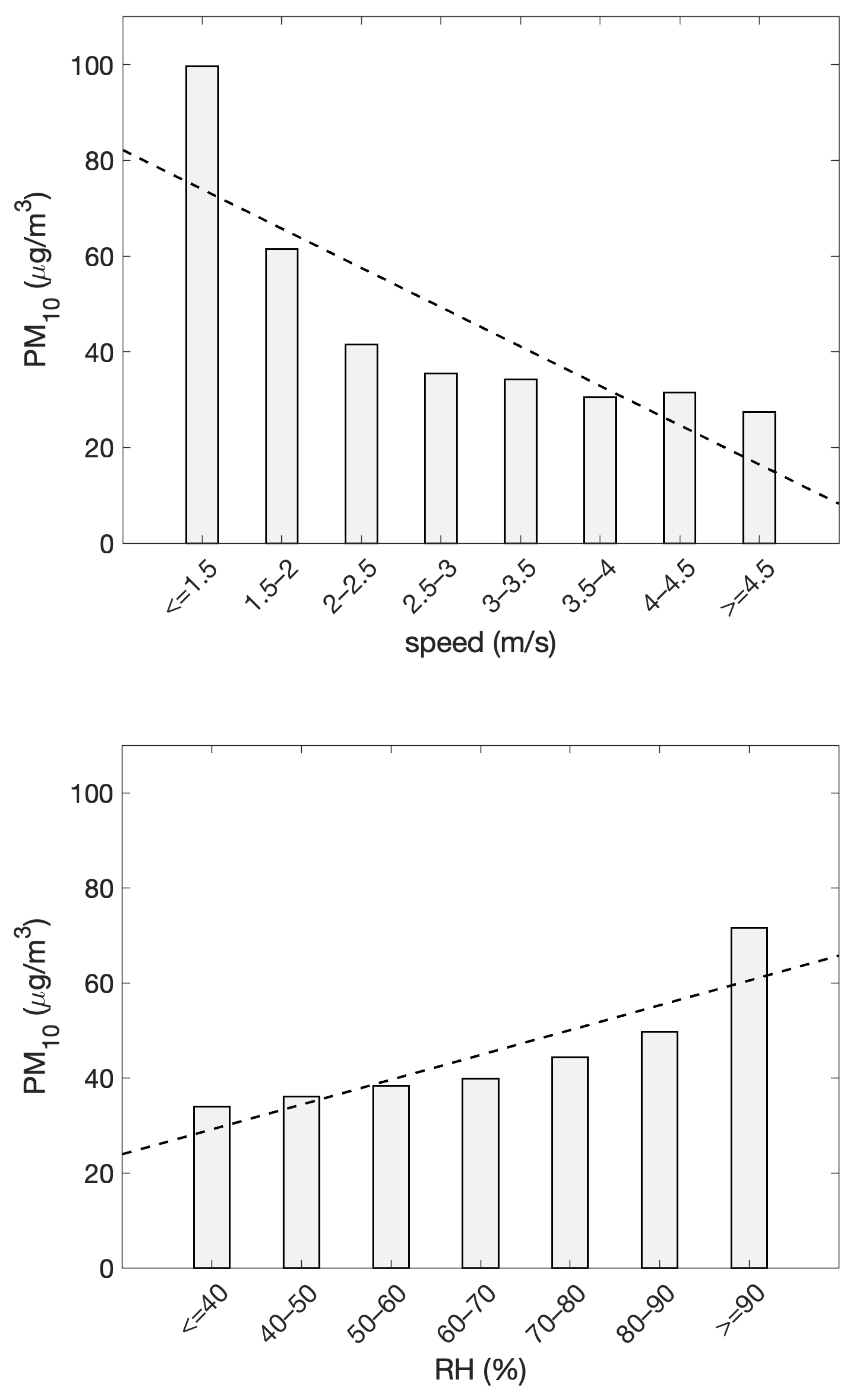
  58. Csavina, J.; Field, J.; Félix, O.; Corral-Avitia, A.Y.; Sáez, A.E.; Betterton, E.A. Effect of wind speed and relative humidity on atmospheric dust concentrations in semi-arid climates. Sci. Total Environ. 2014, 487, 82–90. [Google Scholar] [CrossRef]
Figure 1. Location of the sampling site in Pomigliano d’Arco (Italy).
Atmosphere 16 00393 g001
Figure 2. Distribution of daily PM10 concentrations for the period 2018–2023 as recorded at the PdA monitoring station.
Atmosphere 16 00393 g002
Figure 3. Yearly evolution of daily PM10 concentrations during the period 2018–2023 as recorded at the PdA station. On each box, the mean level is represented by the black diamond, the central horizontal line indicates the median, and the bottom and top edges of the box indicate the 25th and 75th percentiles, respectively. Lines extend from each box to capture the range of the data within 1.5 times the interquartile range. The most extreme data points that fall outside this range are marked with small dots.
Atmosphere 16 00393 g003
Figure 4. Monthly evolution of daily PM10 concentrations during the period 2018–2023 as recorded at the PdA station. On each box, the mean level is represented by the black diamond, the central horizontal line indicates the median, and the bottom and top edges of the box indicate the 25th and 75th percentiles, respectively. Lines extend from each box to capture the range of the data within 1.5 times the interquartile range. The most extreme data points that fall outside this range are marked with small dots.
Atmosphere 16 00393 g004
Figure 5. Normalized time series at the PdA site. Anomalies (values exceeding the median by more than 1.5 times the interquartile range) are indicated in red.
Atmosphere 16 00393 g005
Figure 6. Trajectory means of airflow patterns arriving at PdA during the period 2018–2023. The percentages represent the frequency of occurrence for each cluster. Symbols corresponding to each trajectory are displayed at intervals of 12 h.
Atmosphere 16 00393 g006
Figure 7. Seasonal frequency of each airflow pattern.
Atmosphere 16 00393 g007
Figure 8. The p d f for residence time (upper-left panel) and its decomposition into directional (upper-right panel) and accumulation potential (lower panel) components.
Atmosphere 16 00393 g008
Figure 9. Ratio of conditional probability, calculated for values above the 80th percentile (upper panel), and below the 20th percentile (lower panel).
Atmosphere 16 00393 g009
Figure 10. PM10 concentrations vs. wind speed (upper panel) and relative humidity (lower panel). The dashed lines represent the linear best fit, highlighting the trend line of particulate matter vs. wind and relative humidity ranks.
Atmosphere 16 00393 g010
Table 1. Pearson correlation coefficients (R) between PM10 concentrations measured at PdA and those of PM10 (fifth column) or PM2.5 (sixth column) measured at nearby stations. All these values are significant (p-value < 0.001 ).
Nearby Stations
CodeLatLonR (PM10)R (PM2.5)
IT1497A40.8636°14.2545°0.560.76
IT1496A40.8492°14.2311°0.690.80
PdA stationIT0898A40.8542°14.2511°0.800.80
IT1491A40.8542°14.2717°0.500.47
IT1493A40.8639°14.3414°0.930.90
Table 2. Median wind speed and RH during ADs (anomalous days) and non-ADs (non-anomalous days). For the definition of anomalous days, see Section 3.2.
Median Wind Speed (m/s)Median RH (%)
ADs1.8075.4
Non-ADs2.5168.5
Disclaimer/Publisher’s Note: The statements, opinions and data contained in all publications are solely those of the individual author(s) and contributor(s) and not of MDPI and/or the editor(s). MDPI and/or the editor(s) disclaim responsibility for any injury to people or property resulting from any ideas, methods, instructions or products referred to in the content.

