The Dual Role of Urban Vegetation: Trade-Offs Between Thermal Regulation and Biogenic Volatile Organic Compound Emissions

Abstract

Under the dual pressures of global warming and accelerated urbanization, urban green spaces (UGS) serve as crucial yet paradoxical elements, alleviating urban heat island (UHI) effects while emitting biogenic volatile organic compounds (BVOCs) that exacerbate air pollution; however, their spatial trade-offs remain underexplored. This study bridges this gap by developing an Urban Heat Mitigation Index (HMI) and a BVOC flux accounting framework integrating remote sensing and field observations. The results showed that (1) the cooling effect exhibits significant spatial heterogeneity, with continuous green networks around West Lake and along the Qiantang River forming efficient cooling corridors (HMI > 0.75), while fragmented green spaces in northeastern areas show weaker cooling effects (HMI < 0.35); (2) BVOC emission intensity displays a “high suburbs-low centers” pattern, with suburban areas emitting 1.9–2.3 times more BVOCs than urban centers, while BVOC-induced PM_2.5 (0.02–0.05 μg m⁻³) and O₃ (12–33 μg m⁻³) concentrations in city centers still pose significant health risks; (3) spatial analysis reveals a weak positive correlation between HMI and BVOC emissions (Moran’s I = 0.096, p < 0.05), with four distinct coupling patterns identified: “high cooling-low emissions” (17.5% of area), “low cooling-high emissions” (1.1%), “high cooling-high emissions” (18.7%), and “low cooling-low emissions” (3.9%). This study provides quantitative evidence for optimizing UGS layouts to balance ecological benefits and environmental risks, emphasizing the importance of vegetation screening and spatial allocation in sustainable urban planning.

1. Introduction

Global warming has become the most serious environmental challenge of the 21st century, with the frequency of extreme heat events posing a direct threat to urban systems [1,2,3]. Concurrent with accelerated urbanization and population concentration [4,5], changes in subsurface properties and vegetation cover [6,7], triggered by land-use changes, have not only significantly reshaped the landscape pattern and surface energy balance of cities, but have also resulted in a significant change in the energy balance of urban landscapes [8] causing multiple environmental effects, including the degradation of ecosystem services [9,10], the intensification of atmospheric pollution [11,12], and the urban heat island (UHI) effect [13,14,15].

Notably, the synergistic effect of the UHI with global warming significantly amplifies heat-related mortality risks, posing a critical challenge to global public health [16,17]. As a core element of blue–green infrastructure, urban green space (UGS) is recognized as the most promising nature-based solution for microclimate regulation through shade effect and transpiration cooling mechanism [18,19,20,21], while delivering additional essential ecosystem services [22,23]. Its cooling effectiveness is co-regulated by patch size, spatial configuration, and characteristics of the surrounding built environment [14,15,24], and this multidimensional dependence has led to the significant spatial heterogeneity of cooling effectiveness among global cities [25].

However, the ecological benefits of UGS are accompanied by countervailing effects. Vegetation-released biogenic volatile organic compounds (BVOCs) initiate photochemical processes that generate ground-level ozone (O₃) and secondary organic aerosols (SOA) [26], significantly contributing to urban O₃ and PM_2.5 pollution episodes [27]. These pollutants increase respiratory and cardiovascular disease mortality [28,29]; O₃ also harms ecosystems by reducing photosynthetic rates and even plant yields [30], a risk that is particularly pronounced at high urban background concentrations [31]. Current studies have focused on the characterization of BVOC emissions at different tree species levels [32,33]; the construction of multi-scale BVOC emission inventories [34], and the contribution of BVOCs to regional atmospheric composite pollution [35]. However, there are significant limitations in the refined spatial characterization of the existing methods [34], which seriously constrain the accurate assessment of urban air quality and public health impacts [36,37,38].

In the context of climate change and UHI synergistically exacerbating health risks, how to weigh the cooling effectiveness of UGS and the risk of BVOC emissions has become a key issue to be solved for sustainable urban development. Taking Hangzhou, China, as a case study, this research innovatively integrates 2020 field observation data with remote sensing techniques. We develop an urban heat mitigation index to quantify UGS cooling effectiveness while employing bottom-up BVOC flux accounting through biogenic emission modeling. Spatial overlay analysis and autocorrelation modeling reveal the geographic coupling between thermal regulation and emission patterns. These methodological advances not only elucidate the complex trade-off mechanism between urban greening benefits and air quality risks but also establish a transferable framework for evidence-based urban planning, providing municipalities like Hangzhou with science-driven strategies to simultaneously address climate adaptation and environmental health challenges.

2. Materials and Methods

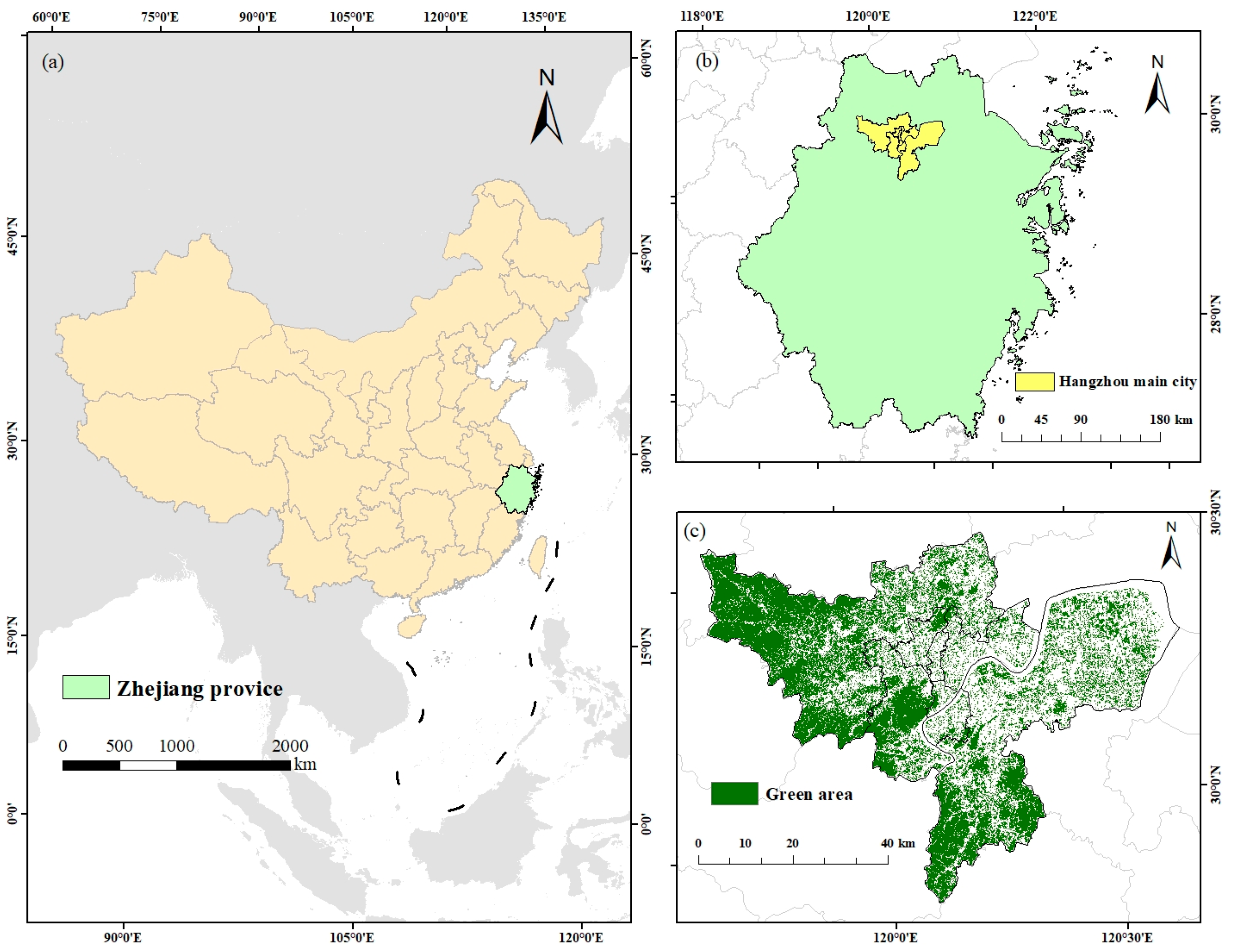
2.1. Study Area

Hangzhou (29°11′ N–30°33′ N, 118°21′ E–120°30′ E) is located in the northern part of China’s southeastern coastal region (Figure 1) and has a subtropical monsoon climate. There are four distinct seasons and abundant rainfall. The average annual temperature of the city is 17.8 °C, and the annual precipitation is 1454 mm. The main vegetation types here are broad-leaved evergreen forests and mixed forests. In recent years, Hangzhou’s green space has been expanding, and from 2010 to 2021, the area of parks and green spaces increased to 11,124 hectares (https://tjj.hangzhou.gov.cn/art/2023/12/4/art_1229453592_4222689.html, accessed 2 February 2025).

2.2. Urban Thermal Mitigation Analysis

The urban cooling model from the integrated valuation of ecosystem services and trade-offs (InVEST) model (https://naturalcapitalproject.stanford.edu/software/invest, accessed 2 February 2025) was used to calculate thermal mitigation in the city. The model first calculates a cooling capacity (CC) index for each pixel based on local shade, evapotranspiration, and albedo. The shade factor represents the proportion of tree canopy (≥2 m in height) associated with each land use/land cover (LULC) category. Potential evapotranspiration (https://data.tpdc.ac.cn, accessed 5 February 2025) and land use (http://www.resdc.cn, accessed 8 February 2025) were resampled in the calculations.

The evapotranspiration index (ETI) represents a normalized value of potential evapotranspiration [39]:

$$ETI={\displaystyle \frac{K_{c}ET0}{{ET}_{max}}}$$

(1)

where K_c is the evapotranspiration coefficient of the crop, ET0 is the reference evapotranspiration (mm), and ET_max is the maximum raster evapotranspiration value (mm). The cooling index CC_i for each pixel is calculated as follows:

$${CC}_i=0.6shade+0.2albedo+0.2\mathrm{E}\mathrm{T}1$$

(2)

where shade is shade and albedo indicate the percentage of reflected solar radiation for that site type (%).

Urban heat mitigation index HMI:

$$HMI=\left\{\begin{array}{c}{CC}_i\hspace{1em}\hspace{1em}\mathrm{i}\mathrm{f}{CC}_i\ge {CC}_{{park}_i}\mathrm{o}\mathrm{r}{GA}_i<2\mathrm{h}\mathrm{a}\\ {CC}_{{park}_i}\hspace{1em}\hspace{1em}\hspace{1em}\mathrm{O}\mathrm{t}\mathrm{h}\mathrm{e}\mathrm{r}\mathrm{s}\mathrm{i}\mathrm{t}\mathrm{u}\mathrm{a}\mathrm{t}\mathrm{i}\mathrm{o}\mathrm{n}\mathrm{s}\hspace{1em}\hspace{1em}\hspace{1em}\hspace{1em}\hspace{1em}\end{array}\right.$$

(3)

where CC_park is a cooling index for each park [40,41]:

$${\mathrm{G}\mathrm{A}}_{\mathrm{i}}={\mathrm{c}\mathrm{e}\mathrm{l}\mathrm{l}}_{\mathrm{a}\mathrm{r}\mathrm{e}\mathrm{a}}\times {\sum }_{\mathrm{j}\in \mathrm{d}\mathrm{r}\mathrm{a}\mathrm{d}\mathrm{i}\mathrm{u}\mathrm{s} \mathrm{f}\mathrm{r}\mathrm{o}\mathrm{m} \mathrm{i}}{\mathrm{g}}_{\mathrm{i}}$$

(4)

$${\mathrm{C}\mathrm{C}}_{{\mathrm{p}\mathrm{a}\mathrm{r}\mathrm{k}}_{\mathrm{i}}}={\sum }_{\mathrm{j}\in \mathrm{d}\mathrm{r}\mathrm{a}\mathrm{d}\mathrm{i}\mathrm{u}\mathrm{s} \mathrm{f}\mathrm{r}\mathrm{o}\mathrm{m} \mathrm{i}}{\mathrm{g}}_{\mathrm{i}}\times {\mathrm{C}\mathrm{C}}_{\mathrm{j}}\times {\mathrm{e}}^{\left({\displaystyle \frac{-\mathrm{d}\left(\mathrm{i},\mathrm{j}\right)}{{\mathrm{d}}_{\mathrm{c}\mathrm{o}\mathrm{o}\mathrm{l}}}}\right)}$$

(5)

where cell_area represents the grid area in hectares, g_i is pixel j is green space or 0 if it is not, d_(i,j) is the distance between pixels i and j, while d_cool denotes the distance over which the green space exerts a cooling effect (m). The distance-weighted average value of CC_i generated by green spaces is calculated based on these parameters.

2.3. Estimation of BVOC Emissions and Related Air Pollution

In this study, BVOCs were categorized as isoprene (E_ISP), monoterpenes (E_MN), sesquiterpenes (E_SQT), and other volatile organic compounds (OVOCs) (E_OVP). The BVOC emissions algorithm are as follows [42,43,44]:

$${\mathrm{E}}_{\mathrm{I}\mathrm{S}\mathrm{P}}={\mathsf{\epsilon }}_{\mathrm{I}\mathrm{S}\mathrm{P}}\mathrm{D}{\mathsf{\gamma }}_{\mathrm{T}}{\mathsf{\gamma }}_{\mathrm{S}}{\mathsf{\gamma }}_{\mathrm{P}}{\mathsf{\gamma }}_{\mathrm{C}}$$

(6)

$$E_{MNS}={\epsilon }_{MNS}D{\gamma }_T{\gamma }_S{\gamma }_P$$

(7)

$${\mathrm{E}}_{\mathrm{M}\mathrm{N}\mathrm{P}}={\mathsf{\epsilon }}_{\mathrm{M}\mathrm{N}\mathrm{P}}\mathrm{D}{\mathsf{\gamma }}_{\mathrm{T}}{\mathsf{\gamma }}_{\mathrm{S}}$$

(8)

$${\mathrm{E}}_{\mathrm{S}\mathrm{Q}\mathrm{T}}={\mathsf{\epsilon }}_{\mathrm{S}\mathrm{Q}\mathrm{T}}\mathrm{D}{\mathsf{\gamma }}_{\mathrm{T}}{\mathsf{\gamma }}_{\mathrm{S}}$$

(9)

$${\mathrm{E}}_{\mathrm{O}\mathrm{V}\mathrm{P}}={\mathsf{\epsilon }}_{\mathrm{O}\mathrm{V}\mathrm{P}}\mathrm{D}{\mathsf{\gamma }}_{\mathrm{T}}{\mathsf{\gamma }}_{\mathrm{S}}$$

(10)

$${\mathrm{E}}_{\mathrm{M}\mathrm{N}}=\mathrm{L}\mathrm{D}\mathrm{F}\times {\mathrm{E}}_{\mathrm{M}\mathrm{N}\mathrm{S}}+\left(1-\mathrm{L}\mathrm{D}\mathrm{F}\right)\times {\mathrm{E}}_{\mathrm{M}\mathrm{N}\mathrm{P}}$$

(11)

where ε represents the basal emission rate (μg C g⁻¹ h⁻¹) under standard conditions, and the photosynthetically active radiation (PAR) is 1000 μmol m⁻² s⁻¹. The Peak leaf biomass (D) (g) for each tree species was calculated from diameter at breast height (DBH) and tree height using the anisotropic growth equation [45]. γ_T, γ_P, and γ_S are the environmental correction factors used to calculate the effects of temperature, light intensity, and seasonal variations on the synthetic emissions, respectively. γ_C is the inhibitory factor for isoprene emissions by CO₂. Air temperature was used to calculate γ_T because the difference between leaf temperature and air temperature within the city is minimal [46]. Photosynthetically active radiation (PAR) and leaf area index (LAI) were used to calculate γ_P; atmospheric CO₂ concentration was used to calculate γ_C. Detailed information can be found in Figure S1.

We used the Fractional Aerosol Coefficient (FAC) and Incremental Reactivity (IR) methods to estimate the air quality impacts of BVOC emissions, such as O₃ and Secondary Organic Aerosols (SOA) [47,48]:

$${\mathrm{O}\mathrm{F}\mathrm{P}}_{\mathrm{i},\mathrm{j}}={\mathrm{M}\mathrm{I}\mathrm{R}}_{\mathrm{i}}\times {\displaystyle \frac{{\mathrm{E}}_{\mathrm{i},\mathrm{j}}\times {\mathsf{\tau }}_{{\mathrm{O}}_3}}{{\mathrm{S}}_{\mathrm{i}}\times \mathrm{H}}}$$

(12)

$${\mathrm{S}\mathrm{O}\mathrm{A}}_{\mathrm{i},\mathrm{j}}={\mathrm{F}\mathrm{A}\mathrm{C}}_{\mathrm{i}}\times {\displaystyle \frac{{\mathrm{E}}_{\mathrm{i},\mathrm{j}}\times {\mathsf{\tau }}_{\mathrm{S}\mathrm{O}\mathrm{A}}}{{\mathrm{S}}_{\mathrm{i}}\times \mathrm{H}}}$$

(13)

where E_i,j represents the BVOC emissions estimated; S is the area of grid i (30 m × 30 m); τ is the atmospheric lifetime of SOA or O₃. MIR (g O₃/g VOC) denotes the maximum incremental reactivity of the species i. FAC is the aerosol formation coefficient (g SOA/g VOC) and H is the boundary layer height estimated from hourly surface meteorological observations. Specific detailed information can be found in Table S2.

2.4. Spatial Autocorrelation

The autocorrelation model and spatial superposition were used to analyze the spatial relationship between BVOC and HMI to reveal the geographic coupling between the cooling effect of UGS and the risk of BVOC emissions, and to identify the high-risk areas, which will provide a basis for public health interventions [49]. Among them, the autocorrelation model used the bivariate Moran’s I index in geoda [50]:

$$\mathrm{I}={\displaystyle \frac{{\sum }_{\mathrm{i}=1}^{\mathrm{n}}{\sum }_{\mathrm{j}=1}^{\mathrm{n}}{\mathrm{W}}_{\mathrm{i}\mathrm{j}}\left({\mathrm{x}}_{\mathrm{i}}-\overline{\mathrm{x}}\right)\left({\mathrm{y}}_{\mathrm{j}}-\overline{\mathrm{y}}\right)}{{\mathrm{S}}^2\left({\sum }_{\mathrm{i}}{\sum }_{\mathrm{j}}{\mathrm{w}}_{\mathrm{i}\mathrm{j}}\right)}}$$

(14)

where I is the bivariate global spatial autocorrelation index, i.e., the correlation between the spatial distributions of spatial variables x and y on the whole; n is the total number of spatial units; W_ij is the spatial weight matrix established by the K-neighborhood method; x_i and y_j are the observed values of the independent variable and the dependent variable in spatial units i and j, respectively; and S² is the variance of all samples.

Spatial superposition uses local indicators of spatial association (LISA), which is used to describe the degree of spatial aggregation of values with a certain degree of similarity in the local area around the spatial unit, and to identify different spatial agglomeration patterns that may exist at different spatial locations.

3. Results

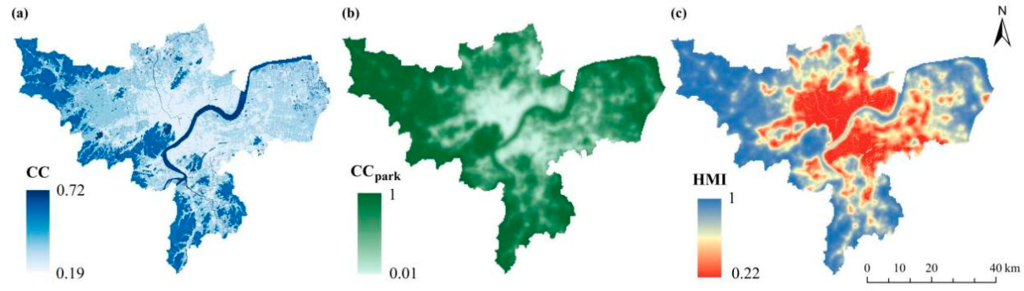
3.1. The Cooling Effect of Green Spaces

The moderating effect of green space on the urban heat link showed significant spatial differentiation (Figure 2). Based on image meta-analysis, vegetation canopy shading, transpiration and surface albedo jointly determined the cooling capacity (Figure 2a), while the cooling effect of each park green space showed a marginal decreasing trend with the expansion of the area (Figure 2b). The HMI composite index (Figure 2c) further indicated that the continuous green space network around West Lake and along the Qiantang River formed efficient cooling corridors (HMI > 0.75), while the northeast part of the city also differed in terms of weaker thermal mitigation due to green space fragmentation (HMI < 0.35), which may be related to the green space area, vegetation type, vegetation cover, and the surrounding environment.

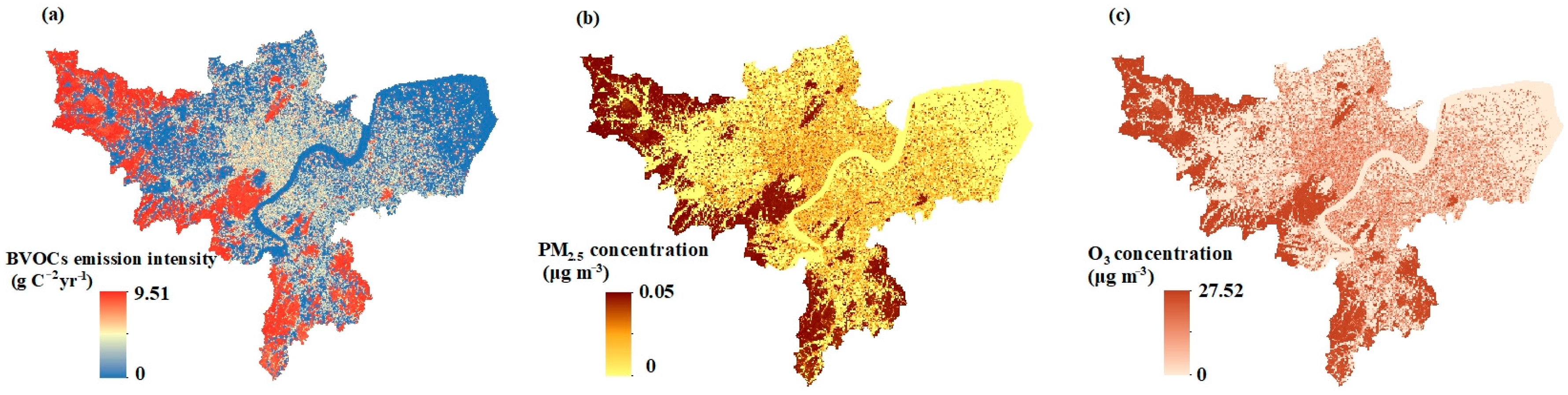
3.2. BVOC Emissions and Air Pollution from Green Spaces

The intensity of BVOC emissions and the air pollution generated were spatially heterogeneous, with high emissions and concentrations concentrated in suburban areas (Figure 3), probably due to the higher vegetation cover in the suburbs, while the concentration of pollutants in urban centers could not be ignored due to the restricted atmospheric diffusion, and the concentrations of PM_2.5 (Figure 3b) and O₃ (Figure 3c) generated by BVOC were not high but the urban areas, with large populations, would cause greater health risks. Although the concentrations of PM_2.5 (Figure 3b) and O₃ (Figure 3c) generated by BVOC are not high, the urban areas are highly populated and cause serious air pollution in the summer, which can lead to greater health risks.

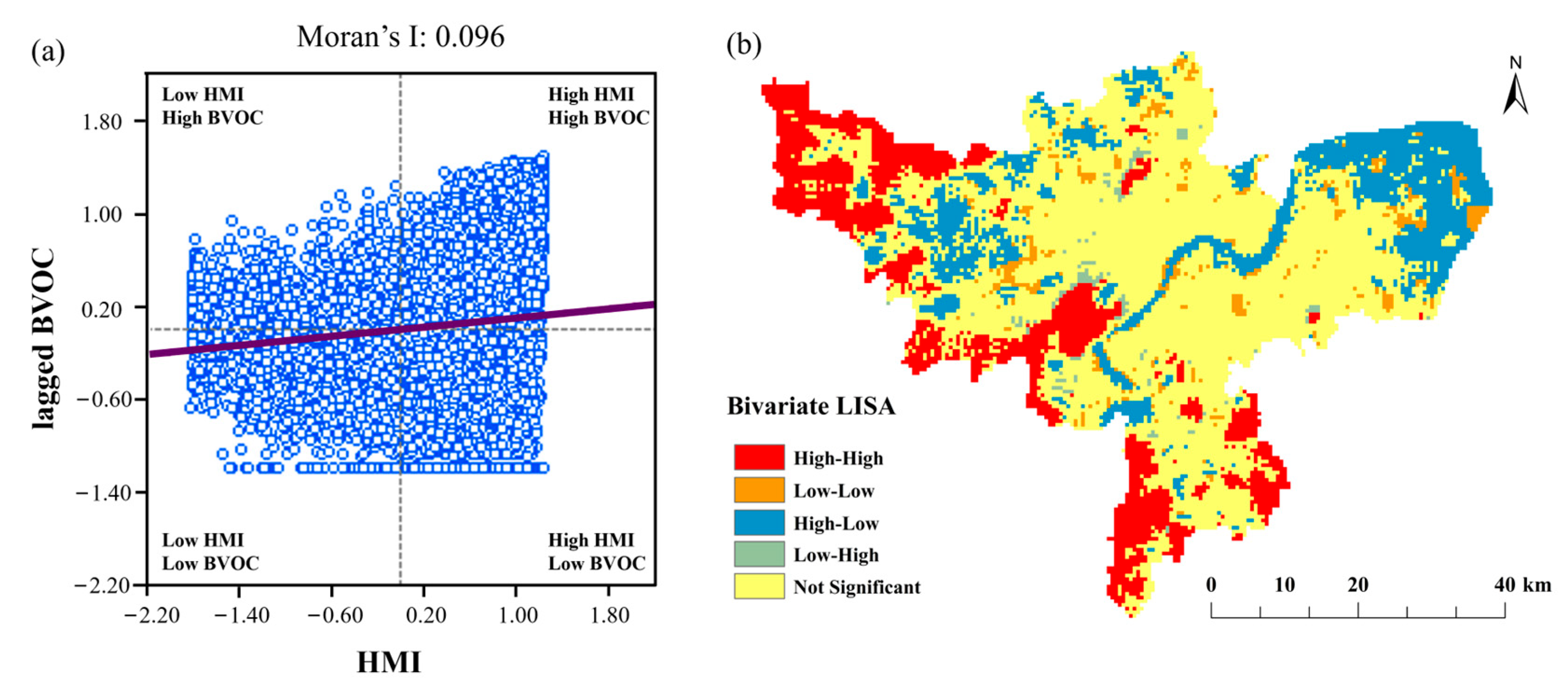
3.3. Spatial Relationships of Greenfield Ecosystem Services

Global spatial autocorrelation analysis showed a weak positive correlation between HMI and BVOC emissions (Moran’s I = 0.096, p < 0.05) (Figure 4a). The Local LISA clustering (Figure 4b) identifies areas that are not correlated (58.8%) as well as four typical types of areas that are correlated: (1) the “high HMI-low BVOC” zone (17.5%), which was concentrated on the southwest side of the West Lake and dominated by transpiration-dominated wetland vegetation; (2) the “low HMI-high BVOC” zone (1.1%), which may be influenced by pine and cypress high-emission tree species; (3) “high HMI-high BVOC” zone (18.7%), which is mostly found in large-scale plantation forests in suburban areas; (4) “low HMI-low BVOC” zone (3.9%), corresponding to hard surfaces in built-up urban areas.

4. Discussion

4.1. Trade-Off Mechanisms and Ecological Regulation of Vegetation Functional Traits

The cooling effects of vegetation and BVOC emissions showed obvious spatial differences, which were closely related to differences in plant functional characteristics [51,52,53]. A clear functional trade-off exists for dominant tree species. For example, although Cinnamomum camphora achieved strong cooling through high transpiration efficiency (average cooling of 0.84 °C per unit area), the intensity of its BVOC emissions was much higher than that of low-emission tree species [54,55,56]. This phenomenon has been related to leaf isoprenoid synthase activity and photosynthetic pathways [32], and C3 plants may mitigate photoinhibition under high-temperature stress by increasing BVOC emissions [33].

In addition, the negative correlation between transpiration efficiency and BVOC emission reveals a dual role of stomatal conductance [57]: large stomatal openings accelerate BVOC volatilization while promoting transpirational cooling. Therefore, tree species with strong stomatal regulation and low BVOC biosynthetic pathways (e.g., Lagerstroemia indica L. and Osmanthus fragrans) and tree species with good cooling effect and low BVOC emissions intensity (e.g., Ilex chinensis and Yulania denudata) were screened as optimization directions [31,58].

4.2. Spatial Coupling Patterns and Optimization Strategies of Cooling and BVOC Emissions

The spatial analysis revealed a weak positive correlation between thermal mitigation effects and BVOC emissions in the study area (Moran’s I = 0.096, p < 0.05), and identified four typical HMI–BVOC emission coupling patterns, which were closely related to the green space structure and vegetation configuration. This result suggests that the nonlinear relationship between green space cooling and emission risk needs to be regulated by refined spatial management.

In the “high cooling-low emission” hotspot (17.5%), which is mainly distributed in the continuous green space network around West Lake and along the Qiantang River, thanks to the complete ecological corridors and reasonable vegetation hierarchies, it is recommended to implement an ecological control red line system to limit the expansion of hard paving, and to increase the efficiency of cooling per unit area by planting a composite layer of trees, shrubs, and grasses. For the “low cooling-high emission” area (1.1%), which mainly occurs in the northeast part of the region with serious green space fragmentation, it is recommended to introduce pollution-resistant, low-emission tree species (e.g., Nerium oleander) to replace the high-emission coniferous species [31], and at the same time, optimize the spatial layout to enhance the connectivity of the green space. The “high cooling-high emission” areas (18.7%) were mainly located in the suburbs, which had a better cooling effect (HMI > 0.65), but the BVOC emission intensity was 1.9–2.3 times higher than that of the urban center. This is mainly related to the vegetation composition dominated by high-emission tree species such as Cinnamomum camphora and Populus tomentosa, and the risk of BVOC emissions should be reduced by adjusting the vegetation structure. The “low cooling—low emission” area (3.9%) is the most widely distributed, mainly in the sporadic green space in the built-up area. Low-emission cooling tree species should be selected to increase the green space coverage and expand the green space area. In addition, a vertical greening structure should be emphasized to improve the efficiency of emission reduction and ecological benefits. It is recommended that BVOC emission intensity be incorporated into the evaluation system of urban green space, and a dynamic monitoring platform be established to track the coupled changes in vegetation physiological parameters and air quality indicators in real time, so as to provide a scientific basis for the sustainable management of urban green space.

4.3. Research Limitations and Future Prospects

This study has limitations regarding model dependency for BVOC emission impacts on air quality, relying on static emission factors and simplified atmospheric chemistry simulations that inadequately capture BVOC–NOx–O₃ dynamics in complex urban environments. This leads to potential ozone formation miscalculations in both urban centers and vegetated suburban areas under varying meteorological conditions. Future research should develop integrated validation systems combining satellite data, ground monitoring networks, and vertical profile observations, while implementing process-based BVOC emission models that account for canopy micrometeorology and plant physiological responses to environmental variations.

Another limitation is the unquantified offsetting effect of anthropogenic heat emissions on green space cooling. This study inadequately addresses thermal contributions from human activities (air conditioning, traffic, and industrial emissions), potentially overestimating vegetation cooling potential in high-density areas, particularly during heat waves. Future work should integrate urban energy models with microclimate simulations, utilizing high-resolution thermal data from mobile platforms and IoT sensors to identify interactions between anthropogenic heat sources and natural cooling processes, thus providing frameworks for coordinated green–gray infrastructure planning.

Health risk assessments in this study exclude cumulative effects from long-term exposure, focusing primarily on acute scenarios while neglecting BVOC-mediated long-term low-dose exposure, particularly for vulnerable populations. This underestimates health considerations in urban greening decisions. Subsequent research should develop health impact assessment frameworks combining cohort tracking with exposure–response modeling, integrating healthcare data and community surveys to establish vulnerability indices for precision urban greening, while conducting multi-year monitoring to quantify long-term as so quantify long-term associations between BVOC emissions and health outcomes.

5. Conclusions

This study reveals the spatial trade-off relationship between heat mitigation and BVOC emissions in urban green spaces, and the main conclusions are as follows: the cooling effectiveness of green spaces is significantly affected by vegetation type, green space size, and spatial configuration. HMI is positively correlated with BVOC emissions, but also negatively correlated in some areas, and an increase in the cooling efficacy can be achieved through vegetation screening and spatial optimization while reducing the amount of pollution generated. It is recommended that cities establish a multi-dimensional evaluation system of “vegetation function—microclimate—air quality” in green space planning and incorporate BVOC emissions into urban ecological assessment indicators.

References

1. Robinson, A.; Lehmann, J.; Barriopedro, D.; Rahmstorf, S.; Coumou, D. Increasing Heat and Rainfall Extremes Now Far Outside the Historical Climate. NPJ Clim. Atmos. Sci. 2021, 4, 51. [Google Scholar] [CrossRef]
2. Sharma, A.; Dutta, P.; Shah, P.; Iyer, V.; He, H.; Sapkota, A.; Gao, C.S.; Wang, Y.C. Characterizing the Effects of Extreme Heat Events on All-Cause Mortality: A Case Study in Ahmedabad City of India, 2002–2018. Urban Clim. 2024, 54, 101832. [Google Scholar] [CrossRef]
3. Matthews, T.; Raymond, C.; Foster, J.; Baldwin, J.W.; Ivanovich, C.; Kong, Q.; Kinney, P.; Horton, R.M. Mortality Impacts of the Most Extreme Heat Events. Nat. Rev. Earth Environ. 2025, 6, 193–210. [Google Scholar] [CrossRef]
4. Sun, L.Q.; Chen, J.; Li, Q.L.; Huang, D. Dramatic Uneven Urbanization of Large Cities Throughout the World in Recent Decades. Nat. Commun. 2020, 11, 5366. [Google Scholar] [CrossRef] [PubMed]
5. Hu, Y.n.; Connor, D.S.; Stuhlmacher, M.; Peng, J.; Turner II, B.L. More Urbanization, More Polarization: Evidence from Two Decades of Urban Expansion in China. NPJ Urban Sustain. 2024, 4, 33. [Google Scholar] [CrossRef]
6. Gao, J.; O’Neill, B.C. Mapping Global Urban Land for the 21st Century with Data-Driven Simulations and Shared Socioeconomic Pathways. Nat. Commun. 2020, 11, 2302. [Google Scholar] [CrossRef]
7. Liu, Z.T.; Wu, R.; Chen, Y.X.; Fang, C.L.; Wang, S.J. Factors of Ecosystem Service Values in a Fast-Developing Region in China: Insights from the Joint Impacts of Human Activities and Natural Conditions. J. Clean. Prod. 2021, 297, 126588. [Google Scholar] [CrossRef]
8. Xiao, R.; Yin, H.Y.; Liu, R.X.; Zhang, Z.H.; Chinzorig, S.; Qin, K.; Tan, W.F.; Wan, Y.; Gao, Z.; Xu, C.; et al. Exploring the Relationship Between Land Use Change Patterns and Variation in Environmental Factors Within Urban Agglomeration. Sustain. Cities Soc. 2024, 108, 105447. [Google Scholar] [CrossRef]
9. Cao, W.; Wu, D.; Huang, L.; Liu, L.L. Spatial and Temporal Variations and Significance Identification of Ecosystem Services in the Sanjiangyuan National Park, China. Sci. Rep. 2020, 10, 6151. [Google Scholar] [CrossRef]
10. Cumming, G.S.; Buerkert, A.; Hoffmann, E.M.; Schlecht, E.; von Cramon-Taubadel, S.; Tscharntke, T. Implications of Agricultural Transitions and Urbanization for Ecosystem Services. Nature 2014, 515, 50–57. [Google Scholar] [CrossRef]
11. Jerrett, M. Atmospheric Science the Death Toll from Air-Pollution Sources. Nature 2015, 525, 330–331. [Google Scholar] [CrossRef] [PubMed]
12. Xu, T.T.; Song, Y.; Liu, M.X.; Cai, X.H.; Zhang, H.S.; Guo, J.P.; Zhu, T. Temperature Inversions in Severe Polluted Days Derived from Radiosonde Data in North China from 2011 to 2016. Sci. Total Environ. 2019, 647, 1011–1020. [Google Scholar] [CrossRef] [PubMed]
13. Ebi, K.L.; Capon, A.; Berry, P.; Broderick, C.; de Dear, R.; Havenith, G.; Honda, Y.; Kovats, R.S.; Ma, W.; Malik, A.; et al. Hot Weather and Heat Extremes: Health Risks. Lancet 2021, 398, 698–708. [Google Scholar] [CrossRef]
14. Wang, J.; Chen, Y.; Liao, W.L.; He, G.H.; Tett, S.F.B.; Yan, Z.W.; Zhai, P.M.; Feng, J.M.; Ma, W.J.; Huang, C.R.; et al. Anthropogenic Emissions and Urbanization Increase Risk of Compound Hot Extremes in Cities. Nat. Clim. Change 2021, 11, 1084–1089. [Google Scholar] [CrossRef]
15. Huang, Q.Y.; Xu, C.; Haase, D.; Teng, Y.M.; Su, M.R.; Yang, Z.F. Heterogeneous Effects of the Availability and Spatial Configuration of Urban Green Spaces on Their Cooling Effects in China. Environ. Int. 2024, 183, 108385. [Google Scholar] [CrossRef] [PubMed]
16. Patz, J.A.; Campbell-Lendrum, D.; Holloway, T.; Foley, J.A. Impact of Regional Climate Change on Human Health. Nature 2005, 438, 310–317. [Google Scholar] [CrossRef]
17. Ward, K.; Lauf, S.; Kleinschmit, B.; Endlicher, W. Heat Waves and Urban Heat Islands in Europe: A Review of Relevant Drivers. Sci. Total Environ. 2016, 569, 527–539. [Google Scholar] [CrossRef]
18. Pataki, D.E.; McCarthy, H.R.; Litvak, E.; Pincetl, S. Transpiration of Urban Forests in the Los Angeles Metropolitan Area. Ecol. Appl. 2011, 21, 661–677. [Google Scholar] [CrossRef]
19. Yang, L.; Liu, X.D.; Qian, F. Research on Water Thermal Effect on Surrounding Environment in Summer. Energy Build. 2020, 207, 109613. [Google Scholar] [CrossRef]
20. Bowler, D.E.; Buyung-Ali, L.; Knight, T.M.; Pullin, A.S. Urban Greening to Cool Towns and Cities: A Systematic Review of the Empirical Evidence. Landsc. Urban Plan. 2010, 97, 147–155. [Google Scholar] [CrossRef]
21. Georgescu, M.; Morefield, P.E.; Bierwagen, B.G.; Weaver, C.P. Urban Adaptation Can Roll Back Warming of Emerging Megapolitan Regions. Proc. Natl. Acad. Sci. USA 2014, 111, 2909–2914. [Google Scholar] [CrossRef] [PubMed]
22. Li, L.; Zheng, M.; Zhang, J.; Li, C.; Ren, Y.; Jin, X.; Chen, J. Effects of green infrastructure on the dispersion of PM2.5 and human exposure on urban roads. Environ. Res. 2023, 223, 115493. [Google Scholar] [CrossRef]
23. Wang, M.; Qin, M.; Xu, P.; Huang, D.; Jin, X.; Chen, J.; Dong, D.; Ren, Y. Atmospheric particulate matter retention capacity of bark and leaves of urban tree species. Environ. Pollut. 2024, 342, 123109. [Google Scholar] [CrossRef] [PubMed]
24. Das, M.; Das, A.; Momin, S. Quantifying the Cooling Effect of Urban Green Space: A Case from Urban Parks in a Tropical Mega Metropolitan Area (India). Sustain. Cities Soc. 2022, 87, 104062. [Google Scholar] [CrossRef]
25. Li, Y.X.; Svenning, J.C.; Zhou, W.Q.; Zhu, K.; Abrams, J.F.; Lenton, T.M.; Ripple, W.J.; Yu, Z.W.; Teng, S.N.; Dunn, R.R.; et al. Green Spaces Provide Substantial but Unequal Urban Cooling Globally. Nat. Commun. 2024, 15, 7108. [Google Scholar] [CrossRef]
26. Mochizuki, T.; Miyazaki, Y.; Ono, K.; Wada, R.; Takahashi, Y.; Saigusa, N.; Kawamura, K.; Tani, A. Emissions of Biogenic Volatile Organic Compounds and Subsequent Formation of Secondary Organic Aerosols in a Larix Kaempferi Forest. Atmos. Chem. Phys. 2015, 15, 12029–12041. [Google Scholar] [CrossRef]
27. Huang, R.J.; Zhang, Y.L.; Bozzetti, C.; Ho, K.F.; Cao, J.J.; Han, Y.M.; Daellenbach, K.R.; Slowik, J.G.; Platt, S.M.; Canonaco, F.; et al. High secondary aerosol contribution to particulate pollution during haze events in China. Nature 2014, 514, 218–222. [Google Scholar] [CrossRef]
28. Pugh, T.A.M.; MacKenzie, A.R.; Whyatt, J.D.; Hewitt, C.N. Effectiveness of Green Infrastructure for Improvement of Air Quality in Urban Street Canyons. Environ. Sci. Technol. 2012, 46, 7692–7699. [Google Scholar] [CrossRef]
29. Wang, Y.; Yang, Y.J.; Yuan, Q.Q.; Li, T.W.; Zhou, Y.; Zong, L.; Wang, M.Y.; Xie, Z.Y.; Ho, H.C.; Gao, M.; et al. Substantially Underestimated Global Health Risks of Current Ozone Pollution. Nat. Commun. 2025, 16, 102. [Google Scholar] [CrossRef]
30. Agyei, T.; Juráň, S.; Edwards-Jonášová, M.; Fischer, M.; Švik, M.; Komínková, K.; Ofori-Amanfo, K.K.; Marek, M.V.; Grace, J.; Urban, O. The Influence of Ozone on Net Ecosystem Production of a Ryegrass–Clover Mixture Under Field Conditions. Atmosphere 2021, 12, 1629. [Google Scholar] [CrossRef]
31. Ren, Y.; Qu, Z.L.; Du, Y.Y.; Xu, R.H.; Ma, D.P.; Yang, G.F.; Shi, Y.; Fan, X.; Tani, A.; Guo, P.P.; et al. Air Quality and Health Effects of Biogenic Volatile Organic Compounds Emissions from Urban Green Spaces and the Mitigation Strategies. Environ. Pollut. 2017, 230, 849–861. [Google Scholar] [CrossRef]
32. Guenther, A.B.; Jiang, X.; Heald, C.L.; Sakulyanontvittaya, T.; Duhl, T.; Emmons, L.K.; Wang, X. The Model of Emissions of Gases and Aerosols from Nature Version 2.1 (Megan2.1): An Extended and Updated Framework for Modeling Biogenic Emissions. Geosci. Model Dev. 2012, 5, 1471–1492. [Google Scholar] [CrossRef]
33. Bao, X.X.; Zhou, W.Q.; Xu, L.L.; Zheng, Z. A Meta-Analysis on Plant Volatile Organic Compound Emissions of Different Plant Species and Responses to Environmental Stress. Environ. Pollut. 2023, 318, 120886. [Google Scholar] [CrossRef] [PubMed]
34. Li, L.Y.; Yang, W.Z.; Xie, S.D.; Wu, Y. Estimations and Uncertainty of Biogenic Volatile Organic Compound Emission Inventory in China for 2008–2018. Sci. Total Environ. 2020, 733, 139301. [Google Scholar] [CrossRef] [PubMed]
35. Cai, B.; Cheng, H.M.; Kang, T.F. Establishing the Emission Inventory of Biogenic Volatile Organic Compounds and Quantifying Their Contributions to O3 and PM2.5 in the Beijing-Tianjin-Hebei region. Atmos. Environ. 2024, 318, 120206. [Google Scholar] [CrossRef]
36. Oderbolz, D.C.; Aksoyoglu, S.; Keller, J.; Barmpadimos, I.; Steinbrecher, R.; Skjoth, C.A.; Plass-Dülmer, C.; Prévôt, A.S.H. A Comprehensive Emission Inventory of Biogenic Volatile Organic Compounds in Europe: Improved Seasonality and Land-Cover. Atmos. Chem. Phys. 2013, 13, 1689–1712. [Google Scholar] [CrossRef]
37. Gu, S.; Guenther, A.; Faiola, C. Effects of Anthropogenic and Biogenic Volatile Organic Compounds on Los Angeles Air Quality. Environ. Sci. Technol. 2021, 55, 12191–12201. [Google Scholar] [CrossRef]
38. Venter, Z.S.; Hassani, A.; Stange, E.; Schneider, P.; Castell, N. Reassessing the Role of Urban Green Space in Air Pollution Control. Proc. Natl. Acad. Sci. USA 2024, 121, e2306200121. [Google Scholar] [CrossRef]
39. Zardo, L.; Geneletti, D.; Pérez-Soba, M.; Van Eupen, M. Estimating the Cooling Capacity of Green Infrastructures to Support Urban Planning. Ecosyst. Serv. 2017, 26, 225–235. [Google Scholar] [CrossRef]
40. Mcdonald, R.; Kroeger, T.; Boucher, T.; Longzhu, W.; Salem, R. Planting Healthy Air: A Global Analysis of the Role of Urban Trees in Addressing Particulate Matter Pollution and Extreme Heat. Environ. Sci. 2016, 128, 136. Available online: https://api.semanticscholar.org/CorpusID:197562156 (accessed on 20 February 2025).
41. Kunapo, J.; Fletcher, T.D.; Ladson, A.R.; Cunningham, L.; Burns, M.J. A spatially Explicit Framework for Climate Adaptation. Urban Water J. 2018, 15, 159–166. [Google Scholar] [CrossRef]
42. Guenther, A.; Baugh, B.; Brasseur, G.; Greenberg, J.; Harley, P.; Klinger, L.; Serca, D.; Vierling, L. Isoprene Emission Estimates and Uncertainties for the Central African Expresso Study Domain. J. Geophys. Res. Atmos. 1999, 104, 30625–30639. [Google Scholar] [CrossRef]
43. Staudt, M.; Bertin, N.; Frenzel, B.; Seufert, G. Seasonal Variation in Amount and Composition of Monoterpenes Emitted by Young Pinus pinea Trees—Implications for Emission Modeling. J. Atmos. Chem. 2000, 35, 77–99. [Google Scholar] [CrossRef]
44. Heald, C.L.; Wilkinson, M.J.; Monson, R.K.; Alo, C.A.; Wang, G.; Guenther, A. Response of Isoprene Emission to Ambient CO2 Changes and Implications for Global Budgets. Glob. Change Biol. 2010, 15, 1127–1140. [Google Scholar] [CrossRef]
45. Paul, K.I.; Roxburgh, S.H.; England, J.R.; Ritson, P.I.; Hobbs, T.J.; Brooksbank, K.; Raison, R.J.; Larmour, J.S.; Murphy, S.; Norris, J.; et al. Development and Testing of Allometric Equations for Estimating Above-Ground Biomass of Mixed-Species Environmental Plantings. For. Ecol. Manag. 2013, 310, 483–494. [Google Scholar] [CrossRef]
46. Meier, F.; Scherer, D. Spatial and Temporal Variability of Urban Tree Canopy Temperature During Summer 2010 in Berlin, Germany. Theor. Appl. Climatol. 2012, 110, 373–384. [Google Scholar] [CrossRef]
47. Mentel, T.F.; Kleist, E.; Andres, S.; Dal Maso, M.; Hohaus, T.; Kiendler-Scharr, A.; Rudich, Y.; Springer, M.; Tillmann, R.; Uerlings, R.; et al. Secondary Aerosol Formation from Stress-Induced Biogenic Emissions and Possible Climate Feedbacks. Atmos. Chem. Phys. 2013, 13, 8755–8770. [Google Scholar] [CrossRef]
48. Ghirardo, A.; Xie, J.F.; Zheng, X.H.; Wang, Y.S.; Grote, R.; Block, K.; Wildt, J.; Mentel, T.; Kiendler-Scharr, A.; Hallquist, M.; et al. Urban Stress-Induced Biogenic VOC Emissions and SOA-Forming Potentials in Beijing. Atmos. Chem. Phys. 2016, 16, 2901–2920. [Google Scholar] [CrossRef]
49. Jesri, N.; Saghafipour, A.; Koohpaei, A.; Farzinnia, B.; Jooshin, M.K.; Abolkheirian, S.; Sarvi, M. Mapping and Spatial Pattern Analysis of COVID-19 in Central Iran Using the Local Indicators of Spatial Association (LISA). Bmc Public Health 2021, 21, 2227. [Google Scholar] [CrossRef]
50. Anselin, L. Local Indicators of Spatial Association—LISA. Geogr. Anal. 1995, 27, 93–115. [Google Scholar] [CrossRef]
51. Machado, R.B.; Aguiar, L.M.S.; Jones, G.J.F. Do Acoustic Indices Reflect the Characteristics of Bird Communities in the Savannas of Central Brazil. Landsc. Urban Plan. 2017, 162, 36–43. [Google Scholar]
52. Jerrett, M.; Su, J.G.; MacLeod, K.E.; Hanning, C.; Houston, D.; Wolch, J. Safe Routes to Play? Pedestrian and Bicyclist Crashes Near Parks in Los Angeles. Environ. Res. 2016, 151, 742–755. [Google Scholar] [PubMed]
53. Zhang, L.; Wu, S.; Chang, X.; Wang, X.; Zhao, Y.; Xia, Y.; Trigiano, R.N.; Jiao, Y.; Chen, F. The Ancient Wave of Polyploidization Events in Flowering Plants and Their Facilitated Adaptation to Environmental Stress. Plant Cell Environ. 2020, 48, 2847–2856. [Google Scholar] [CrossRef]
54. Klinger, L.F.; Li, Q.J.; Guenther, A.B.; Greenberg, J.P.; Baker, B.; Bai, J.H. Assessment of Volatile Organic Compound Emissions from Ecosystems of China. J. Geophys. Res. Atmos. 2002, 107, ACH 16-1–ACH 16-21. [Google Scholar] [CrossRef]
55. Ren, Y.; Ge, Y.; Gu, B.J.; Min, Y.; Tani, A.; Chang, J. Role of Management Strategies and Environmental Factors in Determining the Emissions of Biogenic Volatile Organic Compounds from Urban Greenspaces. Environ. Sci. Technol. 2014, 48, 6237–6246. [Google Scholar] [CrossRef]
56. Shao, Y.C.; Zhang, J.C.; Sun, Y.T.; Li, J.; Zhuang, J.Y.; Li, E.; Xue, X. Comparison of Summer Transpiration Characteristics and Cooling and Humidifying Functions of Major Greening Tree Species in Shanghai. Soil Water Conserv. Sci. China 2015, 13, 83–90. [Google Scholar] [CrossRef]
57. Huang, J.B.; Hartmann, H.; Hellén, H.; Wisthaler, A.; Perreca, E.; Weinhold, A.; Rücker, A.; van Dam, N.M.; Gershenzon, J.; Trumbore, S.; et al. New Perspectives on CO2, Temperature, and Light Effects on Bvoc Emissions Using Online Measurements by Ptr-Ms and Cavity Ring Down Spectroscopy. Environ. Sci. Technol. 2018, 52, 13811–13823. [Google Scholar] [CrossRef]
58. Calfapietra, C.; Fares, S.; Manes, F.; Morani, A.; Sgrigna, G.; Sgrigna, G.; Loreto, F. Role of Biogenic Volatile Organic Compounds (BVOC) Emitted by Urban Trees on Ozone Concentration in Cities: A review. Environ. Pollut. 2013, 183, 71–80. [Google Scholar]
Figure 1. Geographic schematic of the study area: (a) Zhejiang Province, China; (b) urban area of Hangzhou City, Zhejiang Province; and (c) distribution of green spaces within the adult area of Hangzhou City.
Atmosphere 16 00385 g001
Figure 2. Cooling effect of green spaces in the study area: (a) cooling per pixel; (b) cooling per park green space; and (c) composite heat mitigation index.
Atmosphere 16 00385 g002
Figure 3. Emission intensity of BVOCs and air pollution generated in the study area: (a) BVOC emission intensity (g C m−2 yr−1); (b) SOA concentration generated by BVOC (μg m−3); and (c) O3 concentration generated by BVOC (μg m−3).
Atmosphere 16 00385 g003
Figure 4. Spatial correlation between HMI and BVOC emissions in the study area: (a) bivariate Moran’s I index; (b) spatial correlation LISA.
Atmosphere 16 00385 g004
Disclaimer/Publisher’s Note: The statements, opinions and data contained in all publications are solely those of the individual author(s) and contributor(s) and not of MDPI and/or the editor(s). MDPI and/or the editor(s) disclaim responsibility for any injury to people or property resulting from any ideas, methods, instructions or products referred to in the content.