Article

A Hybrid VMD-TPE-TCN Framework for Wind Shear Prediction near an Airport Runway

1
Department of Civil, Structural and Environmental Engineering, Trinity College Dublin, D02PN40 Dublin, Ireland
2
Hong Kong Observatory, 134A Nathan Road, Kowloon, Hong Kong, China
3
Key Laboratory of Infrastructure Durability and Operation Safety in Airfield of CAAC, Tongji University, 4800 Cao’an Road, Jiading, Shanghai 201804, China
4
Department of Civil Engineering, College of Engineering, Taif University, P.O. Box 11099, Taif 21944, Saudi Arabia
*
Authors to whom correspondence should be addressed.
Atmosphere 2025, 16(4), 381; https://doi.org/10.3390/atmos16040381
Submission received: 22 February 2025 / Revised: 18 March 2025 / Accepted: 26 March 2025 / Published: 27 March 2025
(This article belongs to the Section Atmospheric Techniques, Instruments, and Modeling)

Abstract

:
Wind shear presents a critical challenge to aviation safety, particularly during aircraft takeoff and landing, necessitating precise and timely forecasting to mitigate operational risks. This paper introduces a hybrid Variational Mode Decomposition (VMD) framework integrated with a Tree-structured Parzen Estimator (TPE)-optimized Temporal Convolutional Network (TCN) for accurate wind shear magnitude prediction. The model utilizes Doppler LiDAR data collected from January 2020 to December 2021 from two Doppler LiDAR systems installed at Hong Kong International Airport (HKIA). The VMD technique decomposes wind shear signals into intrinsic mode functions (IMFs), which are individually modeled using the TCN, effectively capturing both short-term variations and long-term dependencies. TPE-based hyperparameter tuning optimizes key parameters, further enhancing the predictive accuracy of the proposed framework. A comparative evaluation against VMD-TPE-LSTM, VMD-TPE-BiLSTM, VMD-TPE-GRU, and VMD-TPE-BiGRU demonstrates that the VMD-TPE-TCN(IMF 1-2-4-5) framework achieves the best performance. It shows a lower Mean Absolute Error (MAE) of 6.50, Root Mean Square Error (RMSE) of 2.04, and Theil’s U Statistic of 0.1270, reflecting better predictive accuracy. These outcomes affirm the capability of the VMD-TPE-TCN framework to provide reliable wind shear forecasts, enhancing aviation safety, operational planning, and risk management within airport environments.

1. Introduction

Wind shear presents a significant aerodynamic hazard, affecting aircraft stability, imposing structural stresses, and disrupting passenger comfort. The International Civil Aviation Organization (ICAO) recognizes low-level wind shear, which occurs below 1600 feet in altitude and within three nautical miles of the runway threshold, as a major operational risk during takeoff and landing. This atmospheric disturbance can cause sudden changes in wind speed, generate severe turbulence, and disrupt an aircraft’s approach path, often requiring go-arounds and increasing pilot workload [1,2]. 
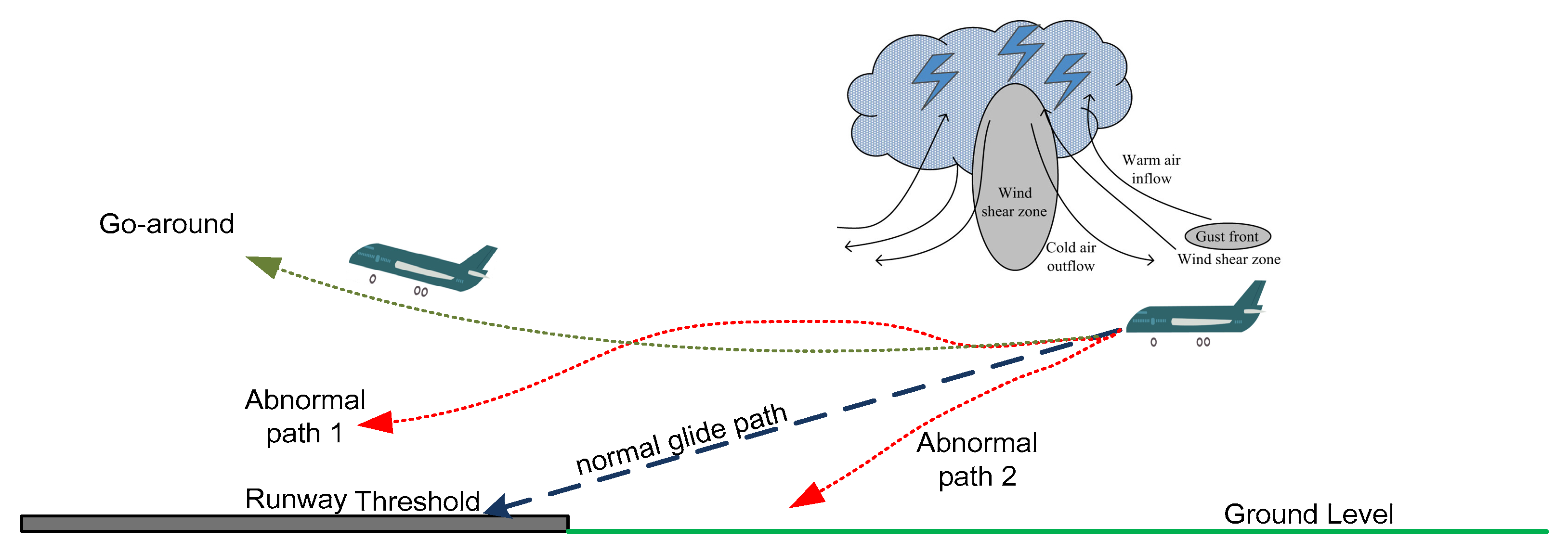
Figure 1 illustrates the impact of wind shear on an approaching aircraft, resulting in potential disruptions such as sudden deviations from the intended glide path and the need for go-arounds. The figure presents a normal glide path along with two abnormal flight paths. In the first case, the aircraft encounters severe wind disturbances, leading to a go-around before reaching the runway threshold. The second occurs due to wind shear-induced loss of altitude, causing a lower-than-expected approach near the runway. These deviations can compromise flight stability, increase pilot workload, and necessitate immediate corrective actions to maintain safe flight operations. The presence of gust fronts, cold air outflows, and turbulence within the wind shear zone further intensifies these challenges, increasing the risk of missed approaches and requiring precise pilot intervention.
The significant impact of wind shear on aviation operations necessitates precise forecasting to enhance flight safety and operational reliability. Accurate prediction allows pilots and air traffic controllers to implement proactive measures, minimizing disruptions and mitigating risks. By anticipating wind shear occurrences, adjustments can be made to flight paths, takeoff and landing schedules, and other operational procedures to ensure safer flight operations. Reliable forecasts enable timely warnings, equipping pilots with critical information to prepare for sudden wind variations and adjust their maneuvers accordingly. This predictive capability reduces the likelihood of wind shear-related incidents and improves overall flight stability.
Wind shear is a transient phenomenon that changes over time and is influenced by dynamic atmospheric conditions [3,4]. Numerous airports globally have gained substantial advantages from the use of precise, high-resolution, remote sensing technologies such as the Terminal Doppler Weather Radar (TDWR) and Doppler Light Detection and Ranging (LiDAR), which are essential for detecting wind shear events. The primary methods for detecting wind shear include TDWR, ground-based anemometer networks, and wind profilers [5,6,7]. Since the mid-1990s, these techniques have been effective in alerting airports to wind shear, especially during tropical cyclones and thunderstorms. However, TDWR systems can be less accurate in clear weather conditions. To address this, the LiDAR system has been integrated with TDWR to enhance the detection and warning capabilities for wind shear in clear weather. Doppler LiDAR can detect return signals from aerosols, providing accurate Doppler wind measurements even in clear air.
Although advanced technologies effectively detect wind shear near airports, they have limitations in predicting its timing and associated risk factors. Accurate wind shear forecasting is essential for improving aviation safety, as it enables timely warnings and the implementation of proactive measures during critical flight phases. Time series modeling is particularly effective for this task, utilizing historical data to analyze and predict wind shear occurrences by identifying temporal patterns and trends. This predictive capability enhances situational awareness, allowing data-driven adjustments to flight operations and reducing the likelihood of wind shear-related incidents [8].
Extensive research has focused on wind speed forecasting within the power and energy sectors, driven by the increasing demand for wind energy generation and advancements in wind energy technology. This body of work is reflected in numerous studies that explore predictive modeling techniques, ranging from statistical methods to machine learning approaches, aimed at improving the accuracy and reliability of wind speed predictions for efficient energy management and grid stability [9,10,11,12]. In contrast, relatively few studies have focused on predicting wind shear events near airport runways. Despite its significant impact on aviation safety, research in this area remains limited, with most efforts directed toward detection rather than prediction. Capturing the complex atmospheric dynamics that lead to wind shear presents a major challenge, requiring advanced modeling approaches that can accurately forecast its occurrence and intensity. Improved prediction techniques are essential for enhancing flight safety and optimizing operational planning [13,14,15,16]. As a result, wind shear prediction in aviation has received less attention than wind energy forecasting. Recent advancements in Artificial Intelligence (AI) have led to significant improvements in accuracy and efficiency across various aviation applications. Machine learning and deep learning models have been applied to predict and analyze complex meteorological phenomena, including turbulence, wind shear, and storm patterns. These AI-driven forecasts enhance situational awareness for pilots and air traffic controllers, contributing to safer and more efficient flight operations. For instance, in aviation meteorology, AI models have been widely employed to evaluate turbulence and wind shear effects. Hybrid Principal Component Analysis (PCA) and K-Means clustering have been used to assess the impact of turbulence on aircraft performance [17]. For forecasting intense wind shear events, Extreme Gradient Boosting (XGBoost) has demonstrated strong predictive capabilities [8]. The severity classification of wind shear has been achieved using the BalanceCascade framework combined with SHAP analysis, allowing for better interpretability of model predictions [18]. The assessment of flight turbulence using LiDAR data has been explored through a combination of Conditional Generative Adversarial Networks (CGAN) and XGBoost, enhancing the accuracy of turbulence predictions [19]. Similarly, Random Forest (RF) has been applied for real-time diagnosis of turbulence associated with thunderstorms, aiding in better turbulence monitoring and warning systems [20]. In aviation safety, AI-driven techniques have been utilized to predict and mitigate risks associated with flight operations. A hybrid model combining Support Vector Machines (SVM) and Deep Neural Networks (DNN) has been employed for forecasting aviation incident risks [21]. For flight risk identification, clustering algorithms have been used to select the most relevant parameters for risk assessment [22]. To predict aircraft system failures, Multi-Layer Perceptron (MLP) and Support Vector Regression (SVR) models have been implemented, offering accurate failure detection and maintenance insights [23]. Furthermore, Recurrent Neural Networks (RNNs) have been applied to detect anomalies in aircraft data, improving early fault detection and operational reliability [24].
In aviation operations, AI models have been integrated to optimize air traffic management and flight efficiency. RF has been employed to forecast temporal and spatial delay states of air traffic, improving congestion management [25]. To enhance flight delay prediction, an Attention-Based Bidirectional Long Short-Term Memory (AB-LSTM) network has been implemented, providing higher accuracy in delay forecasting [26]. Predicting departure delays at airports has been facilitated using Neural Networks, allowing for better scheduling and resource allocation [27]. Similarly, LSTM models have been utilized to estimate aircraft boarding times at gates, optimizing passenger flow and turnaround efficiency [28]. Furthermore, an Explainable Boosting Machine (EBM) has been applied to predict missed approaches induced by wind shear based on pilot reports (PIREPs), providing an interpretable framework for identifying operational disruptions [29].
Despite these advancements, wind shear forecasting remains a challenging task, requiring more robust predictive models that can effectively capture its complex temporal dependencies. This study aims to develop an advanced wind shear prediction framework that integrates Variational Mode Decomposition (VMD) [30,31], Tree-structured Parzen Estimator (TPE), and Temporal Convolutional Network (TCN) [
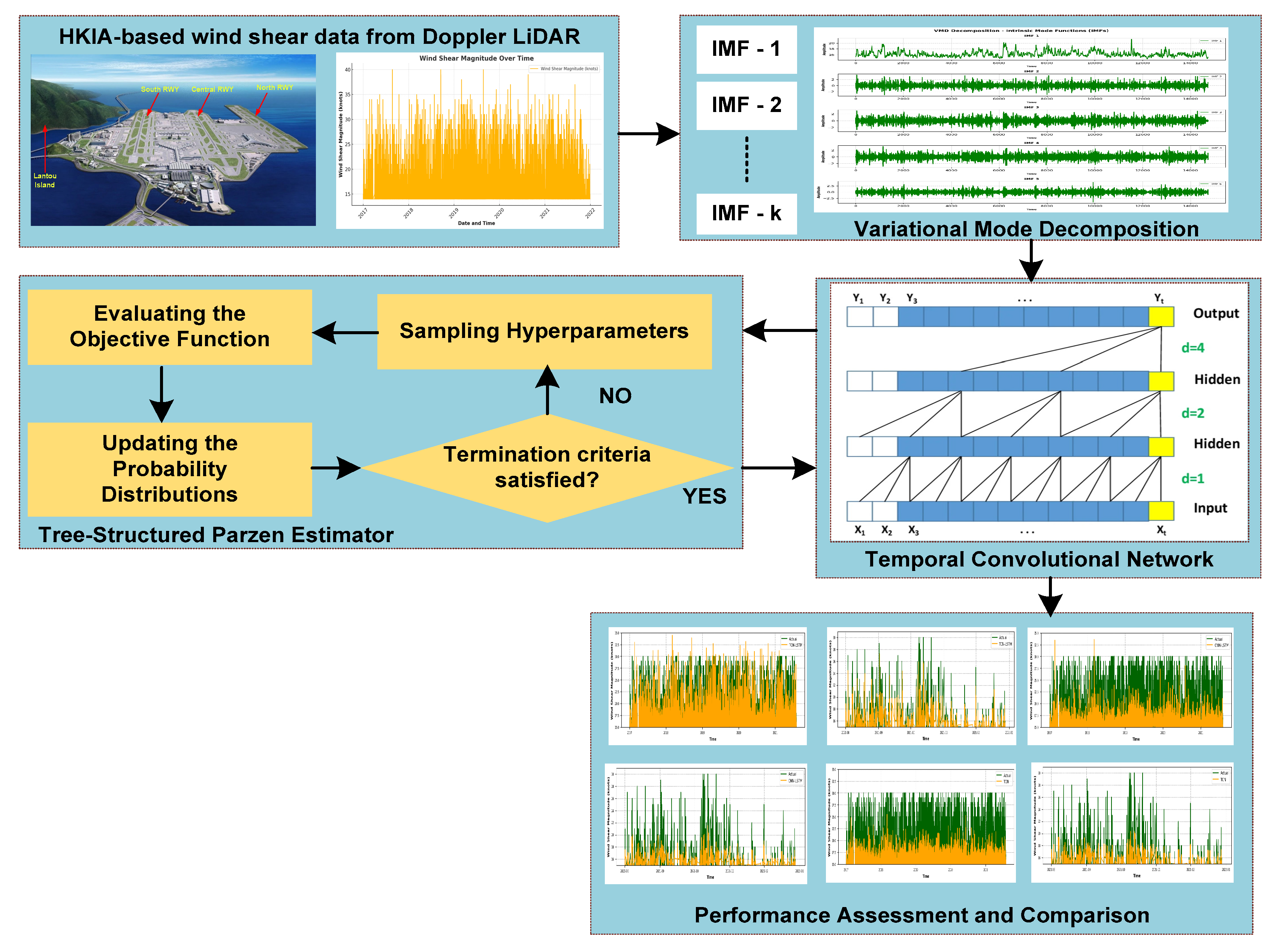
32]. The primary objective is to enhance wind shear forecasting accuracy at Hong Kong International Airport (HKIA) using Doppler LiDAR data. The key research tasks include (1) decomposing wind shear signals into intrinsic mode functions (IMFs) using VMD for better feature extraction; (2) optimizing TCN hyperparameters with TPE to improve predictive performance; (3) evaluating the effectiveness of the proposed VMD-TPE-TCN model against state-of-the-art deep learning models such as LSTM, BiLSTM, and GRU; and (4) assessing the model’s ability to provide reliable forecasts that support aviation safety and operational planning as shown in Figure 2. To the best of our knowledge, this is the first application of a VMD-TPE-TCN framework for wind shear modeling in aviation safety, marking a significant advancement in meteorological forecasting.
The remainder of the paper is organized as follows: Section 2 illustrates detailed information about the study location and HKIA-based Doppler LiDAR data, and provides an overview of the Hybrid VMD-TPE-TCN framework and performance metrics. Section 3 provides a detailed analysis of data including performance assessment. Section 4 concludes by summarizing the findings and future recommendations.

2. Materials and Methods

HKIA functions as the principal aviation gateway for Hong Kong, situated on the artificially expanded Lantau Island along the subtropical coastline of mainland China, as depicted in Figure 3 [33]. It is located at 22.3135° N and 113.9137° E, reinforcing its strategic role as a major hub for international air traffic. Its proximity to key economic centers across the Asia-Pacific region enables extensive global connectivity, supporting both passenger and cargo operations. With state-of-the-art infrastructure, HKIA ranks among the busiest and most efficient airports worldwide. However, the region is prone to severe meteorological disturbances. The airport frequently encounters extreme weather conditions, including typhoons, heavy rainfall, wind shear with speeds between 14 and 30 knots, strong crosswinds, and significant turbulence, all of which pose challenges to runway operations [34,35]. Strong winds flowing across the hills of Lantau Island, situated south of HKIA, are the primary contributors to wind shear and turbulence at the airport. These winds, often associated with tropical cyclones and intense monsoons, account for approximately 75% of all pilot-reported wind shear incidents. Sea breezes contribute to around 15% of these occurrences, while the remaining 10% result from various meteorological phenomena, including gust fronts, microbursts, low-level jets, and turbulence generated by airport structures [36]. These factors emphasize the ongoing need for research to mitigate the effects of severe weather on aviation safety and operational efficiency at HKIA.

2.1. Doppler LiDAR System Description and Data Processing

The Doppler LiDAR system at Hong Kong International Airport (HKIA) is an advanced remote sensing instrument designed to detect and analyze wind shear events. Its initial deployment in August 2002, atop the air traffic control complex, marked the first operational use of Doppler LiDAR for aviation weather alerting worldwide. To enhance coverage and data reliability, a second unit was installed in 2006. The system operates at a 2-micrometer wavelength, emitting laser pulses (≈2 mJ at 500 Hz) and generating line-of-sight velocity measurements (10 Hz) by averaging 50 consecutive pulses per data point, thereby improving measurement precision. It has a 100 m range resolution and can detect wind characteristics within 400 m to 10 km. The maximum measurable velocity is 20 m/s, extendable to 40 m/s with a trade-off in the detection range [37].
To facilitate precise wind shear detection, the Hong Kong Observatory (HKO) developed the Glide Path Scan (GPScan) strategy [38]. This strategy enables Doppler LiDAR to perform targeted scans along three-degree glide paths, aligning laser beams to capture detailed headwind profiles from radial wind measurements as shown in Figure 4 [39]. The system operates within an azimuth range of 220–280° and maintains a fixed 3° elevation angle, allowing for high-resolution wind field representation. Measurements are recorded at slant ranges of 350 to 4500 m, covering critical approach and departure zones. Each LiDAR unit conducts both plan-position indicator (PPI) scans and dedicated glide-path scans, monitoring all major runway configurations: 07LA, 25RA, 07LD, 25RD (North Runway) and 07RA, 25LA, 07RD, 25LD (South Runway). The headwind profiles, derived from radial velocity data, are updated at one-minute intervals [40].
To identify wind shear occurrences, the GLYGA algorithm processes the headwind component profiles, which are gridded at 100 m intervals and extend up to 4–5 nautical miles from the runway endpoint. Utilizing the Peak Spotter algorithm, GLYGA detects sustained velocity changes, identifying wind shear ramps within progressively increasing window lengths of 400, 800, 1600, and up to 6400 m. The severity of these ramps is determined by a severity factor, which scales with headwind increment and the inverse cube root of ramp length. When the severity factor exceeds the operational threshold of 14 knots, an automatic wind shear alert is triggered [18]. Figure 5 depicts an example of Doppler LiDAR velocity plots for RWY 07 and 25 at 0145 UTC, on 27 August 2017.
Table 1 presents key parameters from the Doppler LiDAR system at HKIA, essential for analyzing wind shear events near the runway. The Date and Time indicate when the event was recorded, while Wind Shear Magnitude (knots) quantifies its intensity. The Elevation Angle, fixed at 3.00 degrees, ensures a consistent glide path for approach-phase analysis. The Azimuth Angle represents the LiDAR beam’s horizontal orientation, adjusting across specific degrees for comprehensive runway coverage. The Assigned Runway identifies the detection location, while the Encounter Location specifies the wind shear occurrence location relative to the runway, using codes such as 1MD, RWY, and 2MF (Figure 6). For instance, 1MF denotes an area within 0–1 nautical mile from the runway threshold at the approach (final) end, while 1MD indicates a location within 0–1 nautical mile beyond the runway departure end. The approach glide path remains fixed at 3 degrees, whereas the takeoff profile varies depending on the aircraft type and weight [41].

2.2. Hybrid VMD-TPE-TCN Framework for Time Series Analysis of Wind Shear

The proposed Hybrid VMD-TPE-TCN framework for time series modeling of wind shear integrates Variational Mode Decomposition (VMD), Tree-structured Parzen Estimator (TPE), and Temporal Convolutional Network (TCN) to effectively model wind shear time series data. Wind shear signals exhibit non-stationary and multi-scale characteristics, making them challenging to model using conventional methods. VMD was selected over Empirical Mode Decomposition (EMD) because it addresses key limitations of EMD, such as mode mixing and sensitivity to noise. Unlike EMD, which relies on iterative extrema-based decomposition, VMD formulates the decomposition as a variational optimization problem, ensuring better mode separation and improved robustness in handling non-stationary signals [30,42]. By decomposing the time series into Intrinsic Mode Functions (IMFs), VMD preserves key frequency components while minimizing noise interference. For time series forecasting, TCN was chosen over LSTM and GRU due to its parallelization capability, stable gradients, and superior ability to capture long-range dependencies. Unlike recurrent architectures such as LSTM and GRU, which process data sequentially and suffer from vanishing gradient issues, TCN utilizes dilated causal convolutions to capture both short-term fluctuations and long-term dependencies efficiently [43,44]. This makes TCN computationally more efficient while maintaining high predictive accuracy. Similarly, optimizing TCN requires efficient hyperparameter tuning. TPE is a Bayesian optimization algorithm that models the probability distribution of hyperparameters and iteratively refines the search space. Compared to grid search or random search, TPE reduces computational cost while improving convergence to optimal hyperparameters [32,45]. The steps involved in the proposed framework are as follows:

2.2.1. Step 1: Variational Mode Decomposition (VMD)

The process begins with the VMD step in which a signal processing technique used to decompose the wind shear time series x ( t ) into a set of IMFs, VMD is particularly effective for handling non-stationary and non-linear signals, which, in our case, is wind shear data from Doppler LiDAR. The goal of VMD is to minimize the sum of the bandwidths of the IMFs and ensure that each IMF is compact around a central frequency. This can be achieved by solving an optimization problem using the Alternating Direction Method of Multipliers (ADMM) [46]. The optimization problem is formulated in Equations (1) and (2).
min μ k , ω k k = 1 K t δ t + j π t μ k ( t ) e j ω k t 2 2
Subject to the constraint
k = 1 K μ k t = x ( t ) ,
where μ k t represents the k t h IMF, ω k is its center frequency, t is the partial derivative with respect to time, δ t is the Dirac delta function, ∗ denotes convolution, and j π t represents the Hilbert transform kernel, ensuring analytical signal extraction. The output of this step is a set of IMFs μ k t , which are then used as inputs for the next stage.
A critical challenge in VMD is determining the optimal number of IMFs K, as an arbitrary selection may lead to over-decomposition (excessive noise) or under-decomposition (loss of useful information). To systematically determine k, the Spectral Energy Analysis is employed, which ensures that the chosen number of IMFs retains the majority of the original signal’s energy while avoiding excessive decomposition [47]. To achieve this, we first compute the energy of each IMF, defined as Equation (3).
E k = t I M F k 2 t
where I M F k ( t ) represents the amplitude of the k t h IMF at time t .
The total energy of the decomposed signal across all IMFs is computed by using Equation (5) and the cumulative energy ratio is determined as Equation (5).
E t o t a l = i = 1 K E i
E c u m = i = 1 K E i E t o t a l
The optimal number of IMFs is selected as the smallest K that ensures at least 95% of the total signal energy is captured, preventing unnecessary decomposition while preserving the key features of the wind shear signal.

2.2.2. Step 2: Temporal Convolutional Network (TCN)

The TCN is trained on the optimal decomposed IMFs μ k t . TCN is a specialized neural network designed for sequence modeling tasks, and it uses dilated causal convolutions to capture long-term dependencies in time series data [48]. The causal convolution ensures that the output at time t depends only on inputs at time t and earlier, while the dilated convolution increases the receptive field without increasing the number of parameters. The dilated convolution operation is defined as Equation (6).
f d g t = k = 0 K 1 f ( k ) g t d k
where f is the input signal, g is the filter, and d is the dilation factor. In addition, residual connections are employed to improve gradient flow and enable deeper networks. The output of a residual block is given by Equation (7).
O u t p u t = A c t i v a t i o n C o n v o l u t i o n ( x ) + x
The TCN processes the IMFs and produces a final prediction of the wind shear time series.

2.2.3. Step 3: Tree-Structured Parzen Estimator (TPE)

The hyperparameters of TCN are optimized using the TPE. The TPE is a Bayesian optimization algorithm that efficiently explores the hyperparameter space by modeling the probability distribution of hyperparameters given the validation loss [49]. The algorithm works by constructing two probability models: p x | y , which represents the probability of hyperparameters x given a loss y, and p y , which represents the probability of the loss y. TPE selects hyperparameters that maximize the Expected Improvement (EI) [50], which is given by Equation (8).
E I y ( x ) = y ( y y ) p ( y | x ) d y
where y is a threshold loss value.
This iterative process continues until the optimal hyperparameters for the TCN are found and ensures that the model is well-tuned. In this study, the hyperparameter search was conducted over a predefined range, focusing on parameters that significantly impact model performance, including the number of filters, learning rate, and batch size [51]. These parameters can significantly impact the ability of the model to capture both short-term fluctuations and long-term dependencies in wind shear patterns. For instance, batch size significantly impacts training stability and convergence. Smaller sizes (e.g., 32) enhance generalization but introduce noise, while larger sizes (e.g., 128) stabilize learning but may slow convergence. To optimize training efficiency and model performance, we tuned batch size within the 32–128 range, ensuring a balance between speed, stability, and accuracy. The number of filters is another crucial hyperparameter influencing the ability of the model to extract meaningful temporal features. A lower filter count (50) may limit feature extraction, while a higher count (160) enhances representation but increases computational complexity. To achieve an optimal balance between feature learning and efficiency, we tuned the filter range within 50–160 through hyperparameter optimization. Similarly, the learning rate determines the step size for weight updates during training, directly affecting convergence speed and model stability. A lower learning rate (0.001) ensures stable learning but may slow convergence, while a higher learning rate (0.01) accelerates training but risks instability. To optimize performance, we tuned the learning rate within the range of 0.001–0.01, ensuring a balance between training speed and stability through hyperparameter optimization.

2.2.4. Step 4: Reconstruction and Prediction

The final step involves integrating the outputs of the TCN to produce a comprehensive prediction of the wind shear time series. The decomposed IMFs, each processed by the TCN, are combined to reconstruct the predicted wind shear signal. This can be carried out by using Equation (9).
IMF r e s c a l e d = IMF p r e d - IMF p r e d , m i n MF p r e d , m a x - IMF p r e d , m i n IMF o r i g , m a x - IMF o r i g , m i n + IMF o r i g , m i n
where IMF p r e d is the predicted IMF, IMF p r e d , m i n is the minimum value of the predicted IMF, IMF p r e d , m i n is the maximum value of predicted IMF, and IMF o r i g is the original value of IMF.

2.3. Competitive Models

2.3.1. Long Short-Term Memory (LSTM)

LSTM is an advanced recurrent neural network (RNN) variant designed to handle long-range dependencies more effectively [52]. It achieves this through memory cells and a gating mechanism that selectively retains or forgets information over extended time sequences [53]. In wind shear forecasting, LSTM can capture complex temporal dependencies in Doppler LiDAR data, making it effective for predicting both gradual and abrupt changes in wind shear magnitude. However, LSTM is computationally heavier than GRU, which may impact real-time applications.

2.3.2. Bidirectional Long Short-Term Memory (BiLSTM)

BiLSTM further enhances LSTM by incorporating bidirectional processing [54]. In the case of wind shear modeling, this dual-directionality allows the model to consider both past and future wind patterns, making it particularly useful in capturing dynamic wind shear behaviors. BiLSTM is advantageous when wind shear signals exhibit dependencies that are not strictly forward-propagating, as it can leverage contextual information from future time steps to improve prediction accuracy. However, it also introduces additional computational complexity compared to standard LSTM.

2.3.3. Gated Recurrent Unit (GRU)

GRU is a type of RNN that is well-suited for time-series forecasting due to its ability to capture long-range dependencies while maintaining computational efficiency [55]. Unlike traditional RNNs, GRU uses gates to regulate information flow, preventing vanishing gradient issues. In the context of wind shear prediction, GRU processes sequential Doppler LiDAR data, capturing temporal patterns crucial for forecasting sudden wind shear events. Its relatively simple architecture enables faster training compared to LSTM, making it a competitive choice for real-time applications [56].

2.3.4. Bidirectional Gated Recurrent Unit (BiGRU)

BiGRU extends GRU by incorporating a bidirectional structure, allowing the model to learn from both past and future time steps [57,58]. This is particularly beneficial in wind shear forecasting, as sudden shifts in wind intensity and direction often exhibit patterns that depend on both previous and upcoming conditions. By processing the sequence in both directions, BiGRU enhances pattern recognition and improves the accuracy of wind shear predictions compared to standard GRU.

2.4. Performance Metrics

In the evaluation of the proposed VMD-TPE-TCN time series model, along with other benchmark models, various performance metrics are employed to assess predictive accuracy and effectiveness. These metrics include Mean Squared Error (MSE), Root Mean Square Error (RMSE), and Theil’s U Statistic. MSE and RMSE quantify the magnitude of prediction errors, while Theil’s U provides a comparative measure of forecast accuracy relative to a naïve baseline. These metrics provide a comprehensive evaluation of the model’s performance and ensure a reliable assessment of its suitability for wind shear forecasting. Table 2 presents a detailed overview of these key performance metrics, including their descriptions and mathematical formulations.

3. Results and Discussion

The wind shear dataset from the Doppler LiDAR at HKIA comprises a total of 147,290 wind shear measurements collected from 1 January 2020 to 29 December 2021. These measurements are recorded at irregular intervals, capturing variations that meet or exceed the 14-knot threshold for wind shear events, as defined by the ICAO. Table 3 presents the descriptive statistics for wind shear magnitude, including the minimum, mean, maximum, median, standard deviation (SD), skewness, and kurtosis. For modeling and forecasting, the Doppler LiDAR dataset is split into training and testing sets. The training data include records from 1 January 2020 to 30 July 2021, while the testing dataset consists of observations from 1 August 2021 to 29 December 2021. The implementation was carried out in Python 3.10 on a PC with an Intel(R) Core(TM) i7-6700HQ CPU at 2.6 GHz and 16 GB of RAM, running Windows 10.

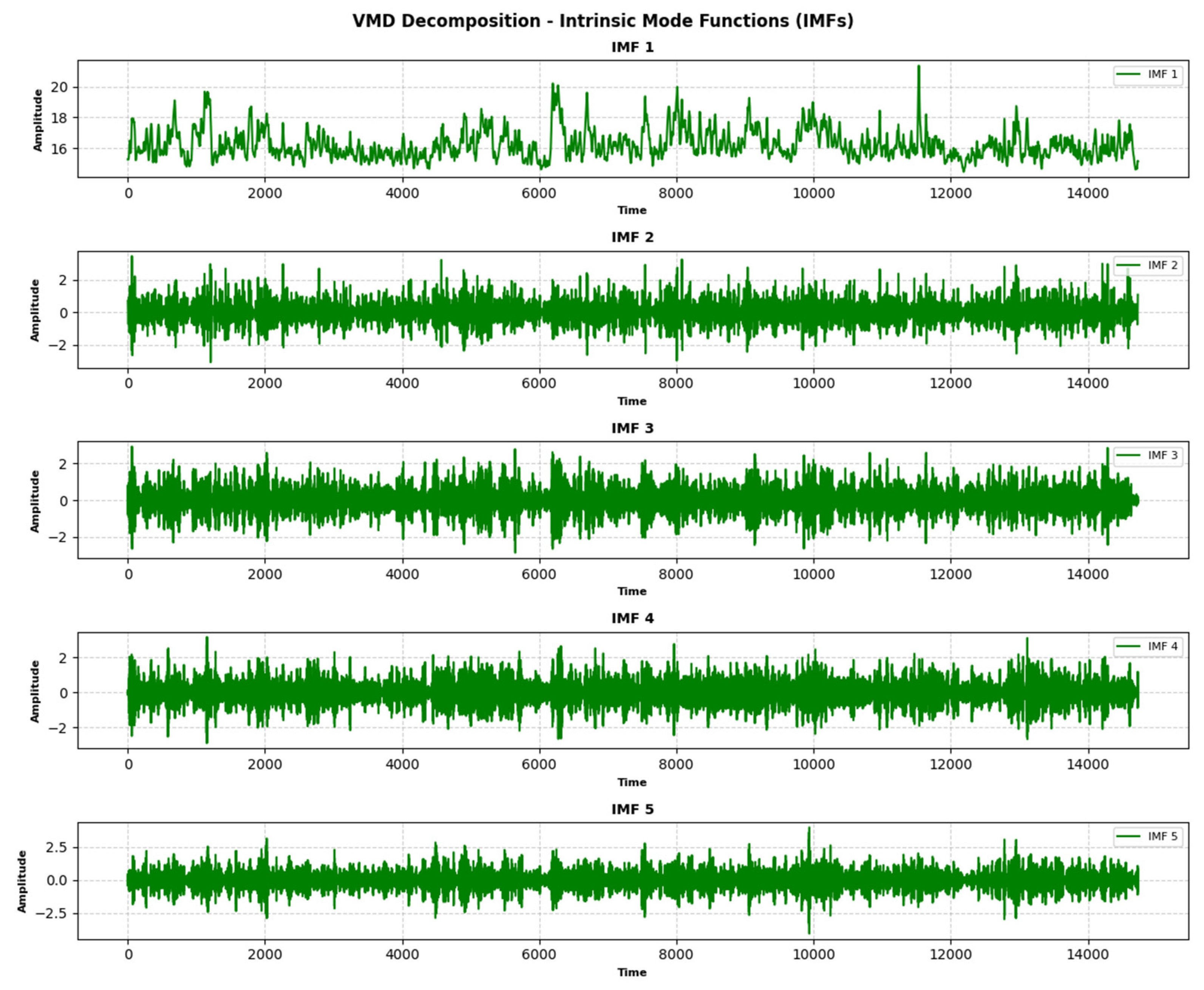
3.1. VMD Decomposition for Wind Shear Magnitude Data

In this study, the VMD technique is employed to decompose the wind shear magnitude time series into a set of IMFs. The wind shear magnitude data, represented by the variable signal, are first downsampled by retaining every 10th data point to reduce computational complexity while preserving the essential characteristics of the signal. The VMD algorithm is then applied with the following parameters: a moderate bandwidth constraint (alpha = 1500), no strict noise tolerance (tau = 0), and an optimized number of IMFs (K = 5) to ensure a concise yet meaningful decomposition. The initialization of frequencies is set to one, and a tolerance level of 1 × 10⁻⁷ is used to ensure convergence. The VMD process decomposes the wind shear magnitude signal into optimized IMFs, each representing distinct frequency components and temporal patterns inherent in the data. The IMFs are plotted individually, with the x-axis representing time and the y-axis representing the amplitude of each IMF. High-frequency IMFs, such as IMF 1 and IMF 2, capture rapid fluctuations or noise in the signal, while low-frequency IMFs, such as IMF 4 and IMF 5, represent slower trends or long-term patterns. This decomposition allows for a detailed analysis of the signal’s multi-scale characteristics, separating it into distinct components, which can be individually analyzed for processing via TPE-optimized TCN. These IMFs are visualized using green lines in subplots, with each subplot corresponding to a specific IMF, as shown in Figure 7.

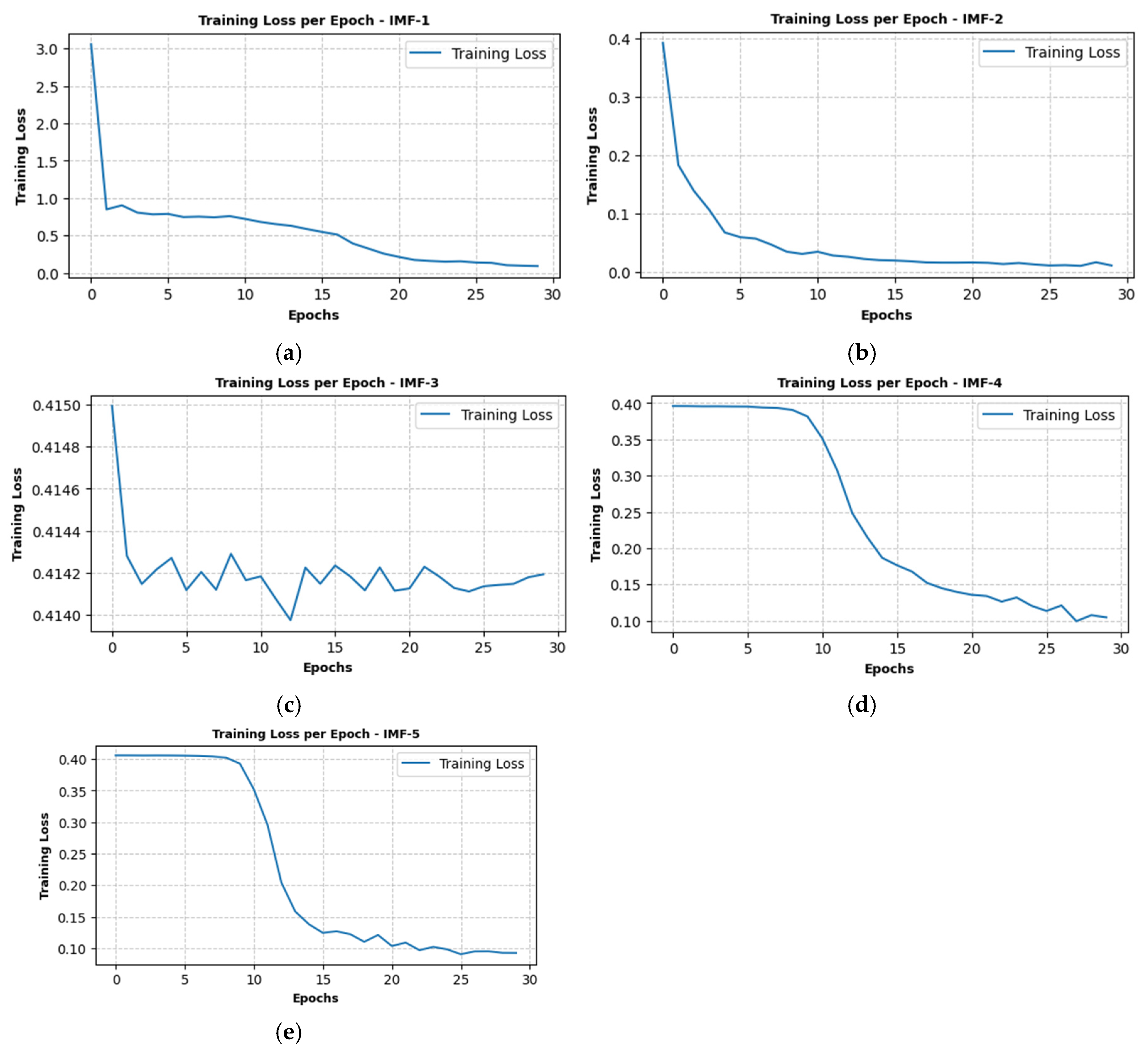
3.2. Training and Hyperparameter Tuning of Each IMF of TCN Model

The process of training and hyperparameter tuning for the TCN model involves several key steps to ensure optimal performance in predicting IMFs derived from wind shear magnitude data. The process begins with the preparation of input–output pairs using a sliding window approach, where a window size of 90 time steps is used to create sequences of input data and corresponding target values for each IMF. This step ensures that the model captures temporal dependencies in the data. Next, hyperparameter optimization is performed using the TPE technique. The hyperparameters optimized include the number of filters, learning rate, and batch size, with the goal of minimizing the MSE loss. The TCN model architecture consists of 1D convolutional layers with dilated causal convolutions, ReLU activation functions, and a global average pooling layer followed by a dense layer for regression. This architecture is designed to effectively capture temporal patterns in the data. Figure 8 shows the training loss per epoch for each IMF. The training loss curves for each IMF are plotted to visualize the model’s convergence during training, showing a steady decrease in loss over epochs.
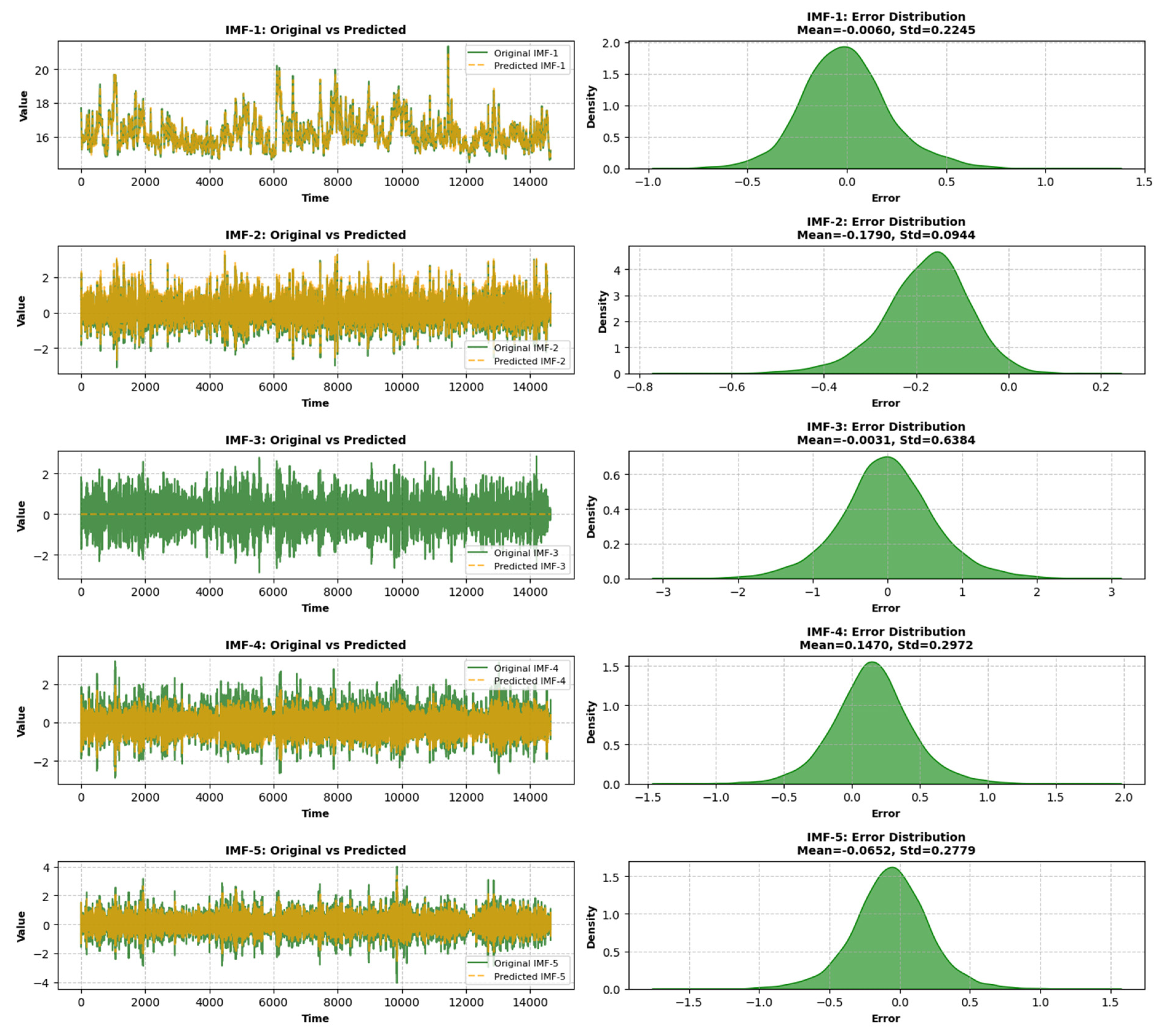
For each IMF, the TCN model is trained using the optimized hyperparameters, and its performance is evaluated using metrics including MSE, RMSE, and Theil’s U Statistic, as shown in Table 4 and Table 5, respectively. Similarly, Figure 9 shows the actual and predicted values of each IMF obtained from the TPE-optimized TCN model. For IMF-1, the optimal hyperparameters are batch size = 32, filters = 128, and learning rate = 0.00167, resulting in excellent predictive accuracy with MSE = 0.020, RMSE = 0.142, and Theil’s U = 0.004. Similarly, for IMF-2, the model achieves strong performance with batch size = 80, filters = 64, and learning rate = 0.00698, yielding MSE = 0.010, RMSE = 0.102, and Theil’s U = 0.076. These results indicate that the TCN model effectively captures high-frequency components of the wind shear data.
For IMF-3, the model shows moderate performance with batch size = 64, filters = 48, and learning rate = 0.00217, producing MSE = 0.035, RMSE = 0.186, and Theil’s U = 0.152. However, the model struggles with low-frequency IMFs, such as IMF-4 and IMF-5. For IMF-4, the optimal hyperparameters are batch size = 80, filters = 64, and learning rate = 0.00145, but the performance metrics are poor, with MSE = 0.391, RMSE = 0.625, and Theil’s U = 0.964. Similarly, for IMF-5, the model achieves sub-optimal results with batch size = 96, filters = 96, and learning rate = 0.00105, resulting in MSE = 0.400, RMSE = 0.632, and Theil’s U = 0.956.

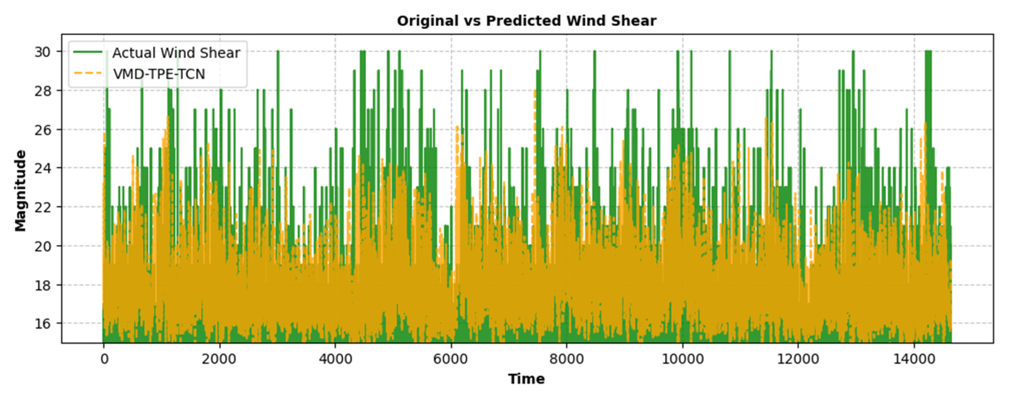
3.3. Rescaling and Reconstruction of Wind Shear Signals

The rescaling and reconstruction process is a critical step in the VMD-TPE-TCN, where the predicted IMFs are rescaled to their original magnitude and combined to reconstruct the wind shear signal. Each predicted IMF is rescaled to match the original scale of the corresponding IMF obtained from VMD. The rescaled IMFs are summed to reconstruct the wind shear signal. However, due to the poor performance of IMF-3, as indicated by its high MSE, RMSE, and Theil’s U values shown in Table 5, it is excluded from the final reconstruction. This exclusion helps improve the overall accuracy of the reconstructed signal by focusing on the well-predicted IMFs (IMF-1, IMF-2, IMF-4, and IMF-5), as shown in Table 6. The actual and predicted wind shear signals are plotted together for comparison, as shown in Figure 10. The actual signal is represented by a solid green line, while the predicted signal from the VMD-TPE-TCN framework is shown as a dashed orange line.

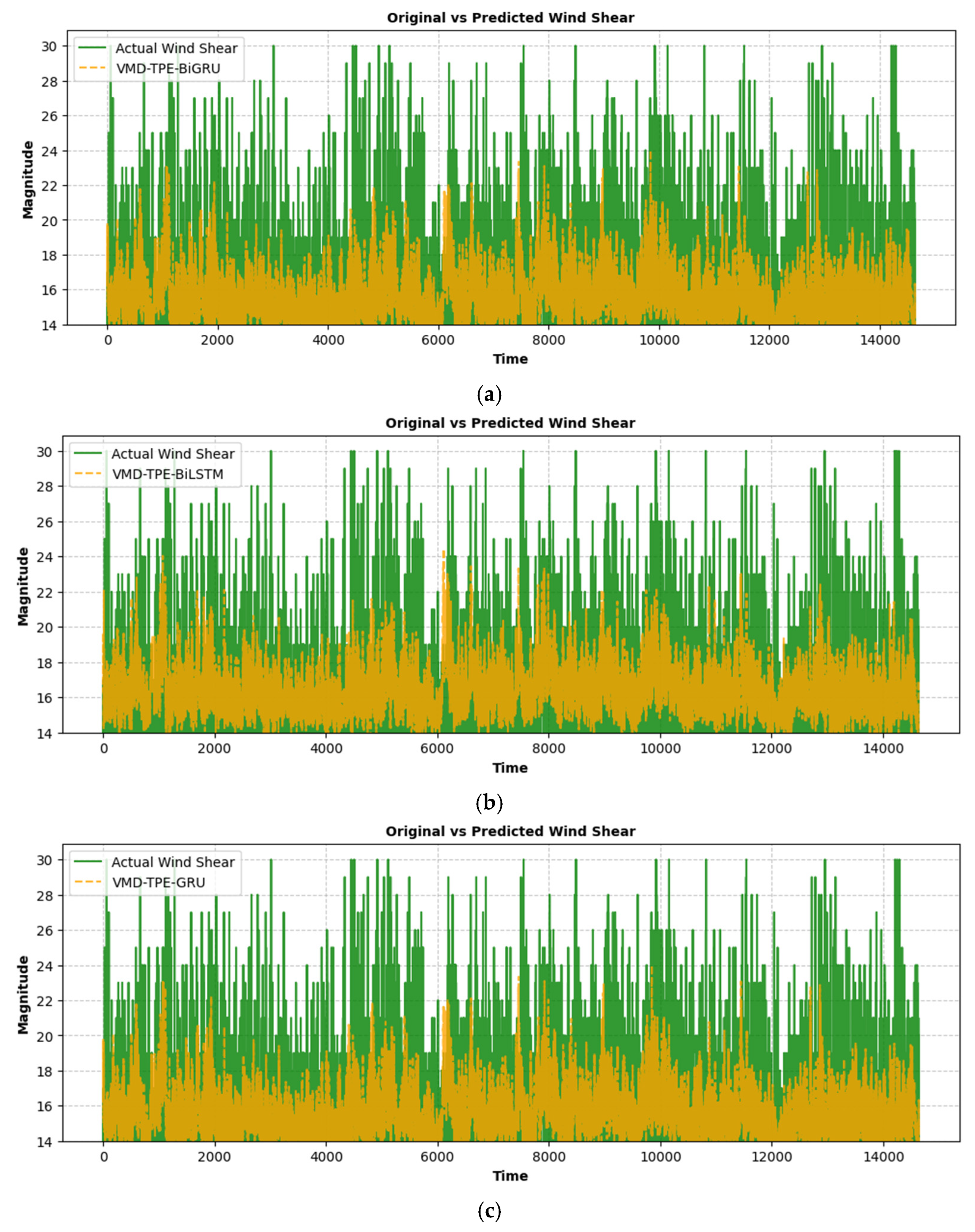
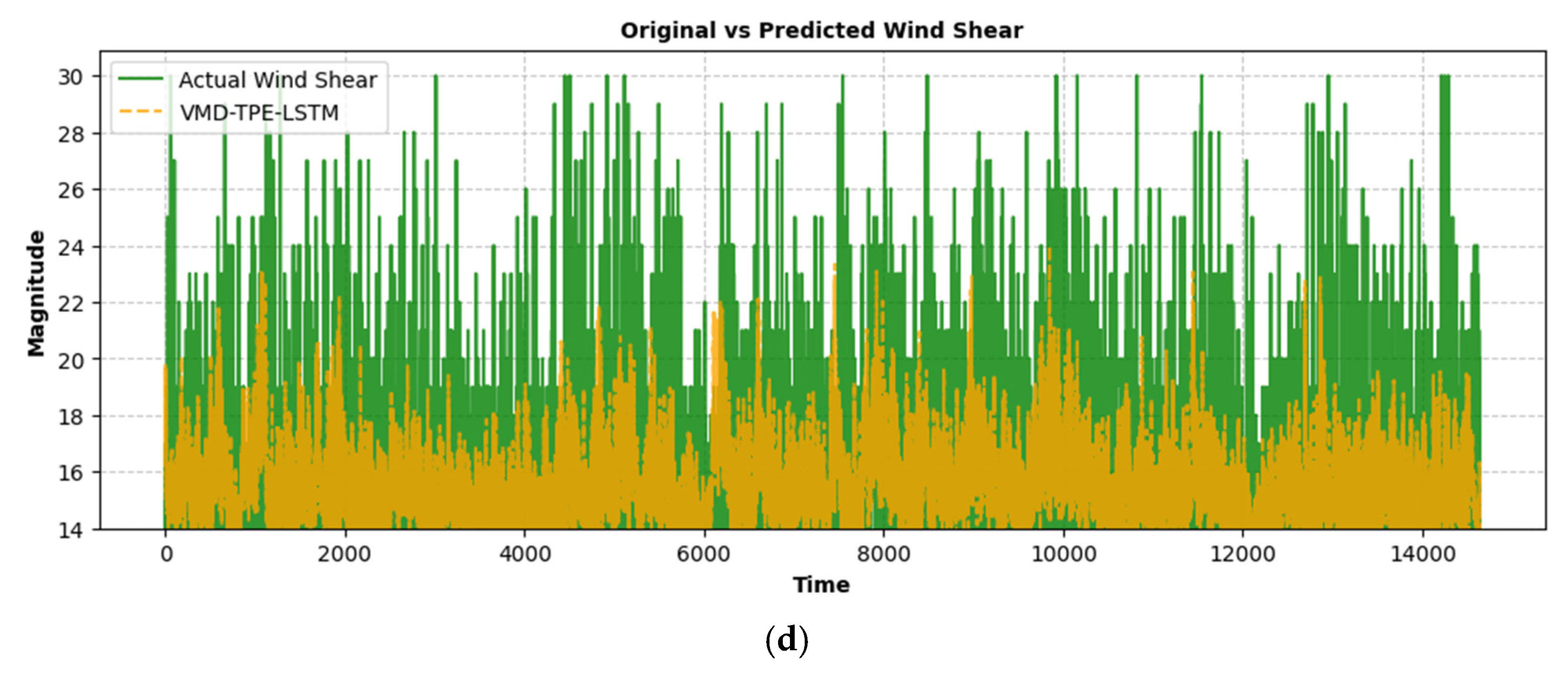
3.4. Comparison with Other Competitive Models

The evaluation of the proposed VMD-TPE-TCN (IMF1-2-4-5) model in comparison with competitive architectures, including VMD-TPE-BiGRU, VMD-TPE-BiLSTM, VMD-TPE-GRU, and VMD-TPE-LSTM, shows its better performance in wind shear magnitude prediction, as shown in Figure 11. The VMD-TPE-TCN model achieves the lowest RMSE (2.04) and Theil’s U (0.1270), indicating higher predictive accuracy and better generalization compared to the other models. In addition, the MAE (6.50) of the VMD-TPE-TCN(IMF1-2-4-5) framework is significantly lower, demonstrating its effectiveness in minimizing absolute prediction errors. The VMD-TPE-BiGRU model is the next best model with RMSE (2.94), Theil’s U (0.1770), and MAE (8.50), as shown in Table 7. A comparative analysis reveals substantial relative improvements achieved by the VMD-TPE-TCN(IMF1-2-4-5) model over other architectures. It achieves an approximate 30.6% reduction in RMSE compared to VMD-TPE-BiGRU, 32.9% compared to VMD-TPE-BiLSTM, and 37.8% compared to VMD-TPE-LSTM. Theil’s U Statistic, which quantifies forecast accuracy relative to a naïve benchmark, is also significantly lower for the VMD-TPE-TCN(IMF1-2-4-5) model, demonstrating a 28.3% improvement over VMD-TPE-BiGRU, 30.7% over VMD-TPE-BiLSTM, and 37.6% over VMD-TPE-LSTM. These outcomes show the ability of the VMD-TPE-TCN(IMF1-2-4-5) framework to capture intricate temporal dependencies more effectively while reducing prediction errors, establishing it as the most reliable model for wind shear forecasting in aviation safety applications.

4. Conclusions and Recommendations

This study proposed a hybrid VMD-TPE-TCN framework for wind shear magnitude forecasting, integrating Variational Mode Decomposition (VMD) for multi-scale signal decomposition and a Tree-structured Parzen Estimator (TPE)-optimized Temporal Convolutional Network (TCN) for enhanced temporal pattern learning. The Doppler LiDAR data from HKIA were used for model training and evaluation. The VMD technique decomposes wind shear signals into Intrinsic Mode Functions (IMFs), allowing TCN to model each IMF individually while TPE optimizes the hyperparameters to refine predictive performance. To validate its effectiveness, the VMD-TPE-TCN framework was compared against alternative models, including VMD-TPE-BiGRU, VMD-TPE-BiLSTM, VMD-TPE-GRU, and VMD-TPE-LSTM. The following conclusions can be drawn:
  • The VMD-TPE-TCN (IMF1-2-4-5) framework demonstrated the best predictive performance among all tested models, achieving an MAE of 6.50, RMSE of 2.04, and Theil’s U Statistic of 0.1270. These results indicate its superior ability to capture temporal dependencies in wind shear data while minimizing forecasting errors.
  • The second-best model, VMD-TPE-BiGRU, recorded an MAE of 8.50, RMSE of 2.94, and Theil’s U Statistic of 0.1770, showing slightly lower predictive accuracy compared to the proposed framework.
  • In contrast, the worst-performing model, VMD-TPE-LSTM, exhibited higher prediction errors, with an MAE of 10.70, RMSE of 3.65, and Theil’s U Statistic of 0.2035, reflecting its reduced effectiveness in modeling wind shear dynamics.
There are certain limitations of this study, which are as follows:
  • The model was trained using Doppler LiDAR data from HKIA, which may restrict its applicability to other airports with different meteorological patterns and geographical conditions.
  • An improper selection of IMFs may lead to over-decomposition or loss of crucial wind shear information, potentially affecting prediction accuracy.
  • Given the dynamic nature of wind shear patterns influenced by climate variability, the current model lacks real-time adaptive learning mechanisms that could enable continuous updating of the forecasting model in response to changing atmospheric conditions.
Future research should focus on expanding the applicability of the VMD-TPE-TCN framework by integrating additional datasets from diverse airport environments to improve generalization. In addition, the integration of real-time adaptive learning mechanisms would enable the model to dynamically adjust to evolving meteorological trends, making wind shear forecasting more responsive and reliable in operational settings.

Author Contributions

Conceptualization, A.K.; Data curation, P.-w.C.; Formal analysis, A.K.; Investigation, F.C.; Methodology, A.K.; Project administration, F.C. and A.H.A.; Resources, P.-w.C.; Software, P.-w.C.; Validation, A.H.A.; Visualization, F.C. All authors have read and agreed to the published version of the manuscript.

Funding

The present study received financial support from the National Natural Science Foundation of China (Grant No. 52250410351), the National Foreign Expert Project (Grant No. QN2022133001L), Taif University (TU-DSPP-2024-173), and Xiaomi Young Talent Program.

Institutional Review Board Statement

Not applicable.

Informed Consent Statement

Not applicable.

Data Availability Statement

The raw data supporting the conclusions of this article will be made available by the authors on request.

Acknowledgments

We are thankful to the Hong Kong Observatory of Hong Kong International Airport for providing us Doppler LiDAR data as well as grateful to Taif University for their valuable support. In addition, we acknowledge the use of the Grammarly AI tool, which was employed solely for grammar correction in the manuscript.

Conflicts of Interest

The authors declare no conflicts of interest.

References

  1. Polukhin, A.; Ostapenko, O. Features of landing approach for aircraft in automatic and yoke control modes in conditions of horizontal lateral wind shear. Наукoємні технoлoгії 2018, 4, 512–517. [Google Scholar]
  2. O’Connor, A.; Kearney, D. Evaluating the effect of turbulence on aircraft during landing and take-off phases. Int. J. Aviat. Aeronaut. Aerosp. 2018, 5, 10. [Google Scholar]
  3. Zhang, H.; Liu, X.; Wang, Q.; Zhang, J.; He, Z.; Zhang, X.; Li, R.; Zhang, K.; Tang, J.; Wu, S. Low-level wind shear identification along the glide path at BCIA by the pulsed coherent doppler LiDAR. Atmosphere 2020, 12, 50. [Google Scholar] [CrossRef]
  4. Bretschneider, L.; Hankers, R.; Schönhals, S.; Heimann, J.-M.; Lampert, A. Wind shear of low-level jets and their influence on manned and unmanned fixed-wing aircraft during landing approach. Atmosphere 2021, 13, 35. [Google Scholar] [CrossRef]
  5. Gheitasi, N.; Mazlumi, F. A review on radar applications in civil aviation. In Proceedings of the International Conference of Iran Air and Space Association, Tehran, Iran, 20–22 May 2023; pp. 1–8. [Google Scholar]
  6. Morris, M.T.; Brewster, K.A.; Carr, F.H. Assessing the Impact of Non-Conventional Radar and Surface Observations on High-Resolution Analyses and Forecasts of a Severe Hailstorm. Electron. J. Sev. Storms Metereology (EJSSM) 2021, 16, 1–39. [Google Scholar] [CrossRef]
  7. Nechaj, P.; Gaál, L.; Bartok, J.; Vorobyeva, O.; Gera, M.; Kelemen, M.; Polishchuk, V. Monitoring of low-level wind shear by ground-based 3D lidar for increased flight safety, protection of human lives and health. Int. J. Environ. Res. Public Health 2019, 16, 4584. [Google Scholar] [CrossRef]
  8. Khattak, A.; Chan, P.-W.; Chen, F.; Peng, H. Time-series prediction of intense wind shear using machine learning algorithms: A case study of Hong Kong international airport. Atmosphere 2023, 14, 268. [Google Scholar] [CrossRef]
  9. Santhosh, M.; Venkaiah, C.; Vinod Kumar, D. Current advances and approaches in wind speed and wind power forecasting for improved renewable energy integration: A review. Eng. Rep. 2020, 2, e12178. [Google Scholar] [CrossRef]
  10. Liu, Z.; Jiang, P.; Zhang, L.; Niu, X. A combined forecasting model for time series: Application to short-term wind speed forecasting. Appl. Energy 2020, 259, 114137. [Google Scholar]
  11. Sweeney, C.; Bessa, R.J.; Browell, J.; Pinson, P. The future of forecasting for renewable energy. Wiley Interdiscip. Rev. Energy Environ. 2020, 9, e365. [Google Scholar]
  12. Zhang, W.; Lin, Z.; Liu, X. Short-term offshore wind power forecasting-A hybrid model based on Discrete Wavelet Transform (DWT), Seasonal Autoregressive Integrated Moving Average (SARIMA), and deep-learning-based Long Short-Term Memory (LSTM). Renew. Energy 2022, 185, 611–628. [Google Scholar]
  13. Zhang, H.; Wu, S.; Wang, Q.; Liu, B.; Yin, B.; Zhai, X. Airport low-level wind shear lidar observation at Beijing Capital International Airport. Infrared Phys. Technol. 2019, 96, 113–122. [Google Scholar] [CrossRef]
  14. Liu, X.; Zhang, H.; Wu, S.; Wang, Q.; He, Z.; Zhang, J.; Li, R.; Liu, S.; Zhang, X. Effects of buildings on wind shear at the airport: Field measurement by coherent Doppler lidar. J. Wind Eng. Ind. Aerodyn. 2022, 230, 105194. [Google Scholar]
  15. Yoshino, K. Low-level wind shear induced by horizontal roll vortices at Narita International Airport, Japan. J. Meteorol. Soc. Jpn. Ser. II 2019, 97, 403–421. [Google Scholar]
  16. Khattak, A.; Zhang, J.; Chan, P.-W.; Chen, F. Assessment of Wind Shear Severity in Airport Runway Vicinity using Interpretable TabNet approach and Doppler LiDAR Data. Appl. Artif. Intell. 2024, 38, 2302227. [Google Scholar]
  17. Mizuno, S.; Ohba, H.; Ito, K. Machine learning-based turbulence-risk prediction method for the safe operation of aircrafts. J. Big Data 2022, 9, 29. [Google Scholar]
  18. Khattak, A.; Chan, P.W.; Chen, F.; Peng, H. Interpretable ensemble imbalance learning strategies for the risk assessment of severe-low-level wind shear based on LiDAR and PIREPs. Risk Anal. 2024, 44, 1084–1102. [Google Scholar]
  19. Zhuang, Z.; Zhang, H.; Chan, P.-W.; Tai, H.; Deng, Z. A Machine Learning-Based Model for Flight Turbulence Identification Using LiDAR Data. Atmosphere 2023, 14, 797. [Google Scholar] [CrossRef]
  20. Williams, J.K. Using random forests to diagnose aviation turbulence. Mach. Learn. 2014, 95, 51–70. [Google Scholar]
  21. Zhang, X.; Mahadevan, S. Ensemble machine learning models for aviation incident risk prediction. Decis. Support Syst. 2019, 116, 48–63. [Google Scholar]
  22. Mangortey, E.; Monteiro, D.; Ackley, J.; Gao, Z.; Puranik, T.G.; Kirby, M.; Pinon-Fischer, O.J.; Mavris, D.N. Application of machine learning techniques to parameter selection for flight risk identification. In Proceedings of the AIAA Scitech 2020 Forum, Orlando, FL, USA, 6–10 January 2020; p. 1850. [Google Scholar]
  23. Celikmih, K.; Inan, O.; Uguz, H. Failure prediction of aircraft equipment using machine learning with a hybrid data preparation method. Sci. Program. 2020, 2020, 8616039. [Google Scholar] [CrossRef]
  24. Nanduri, A.; Sherry, L. Anomaly detection in aircraft data using Recurrent Neural Networks (RNN). In Proceedings of the 2016 Integrated Communications Navigation and Surveillance (ICNS), Herndon, VA, USA, 19–21 April 2016; pp. 5C2-1–5C2-8. [Google Scholar]
  25. Rebollo, J.J.; Balakrishnan, H. Characterization and prediction of air traffic delays. Transp. Res. Part C Emerg. Technol. 2014, 44, 231–241. [Google Scholar] [CrossRef]
  26. Mamdouh, M.; Ezzat, M.; Hefny, H. Improving flight delays prediction by developing attention-based bidirectional LSTM network. Expert Syst. Appl. 2024, 238, 121747. [Google Scholar] [CrossRef]
  27. Khan, W.A.; Ma, H.-L.; Chung, S.-H.; Wen, X. Hierarchical integrated machine learning model for predicting flight departure delays and duration in series. Transp. Res. Part C Emerg. Technol. 2021, 129, 103225. [Google Scholar] [CrossRef]
  28. Schultz, M.; Reitmann, S. Machine learning approach to predict aircraft boarding. Transp. Res. Part C Emerg. Technol. 2019, 98, 391–408. [Google Scholar] [CrossRef]
  29. Khattak, A.; Chan, P.-w.; Chen, F.; Peng, H. Explainable Boosting Machine for Predicting Wind Shear-Induced Aircraft Go-around based on Pilot Reports. KSCE J. Civ. Eng. 2023, 27, 4115–4129. [Google Scholar] [CrossRef]
  30. Lahmiri, S. A variational mode decompoisition approach for analysis and forecasting of economic and financial time series. Expert Syst. Appl. 2016, 55, 268–273. [Google Scholar] [CrossRef]
  31. Chen, H.; Lu, T.; Huang, J.; He, X.; Yu, K.; Sun, X.; Ma, X.; Huang, Z. An improved VMD-LSTM model for time-varying GNSS time series prediction with temporally correlated noise. Remote Sens. 2023, 15, 3694. [Google Scholar] [CrossRef]
  32. Liang, M.; An, B.; Li, K.; Du, L.; Deng, T.; Cao, S.; Du, Y.; Xu, L.; Gao, X.; Zhang, L. Improving genomic prediction with machine learning incorporating TPE for hyperparameters optimization. Biology 2022, 11, 1647. [Google Scholar] [CrossRef]
  33. Yuen, A.; Tsui, K.; Fung, M. Hong Kong Airport’s Competitiveness as an International Hub. In Aviation Law and Policy in Asia; Brill Nijhoff: Leiden, The Netherlands, 2020; pp. 118–142. [Google Scholar]
  34. Chan, P.; Hon, K. Observation and numerical simulation of terrain-induced windshear at the Hong Kong International Airport in a planetary boundary layer without temperature inversions. Adv. Meteorol. 2016, 2016, 1454513. [Google Scholar] [CrossRef]
  35. Hon, K.; Chan, P. Application of LIDAR-derived eddy dissipation rate profiles in low-level wind shear and turbulence alerts at Hong Kong International Airport. Meteorol. Appl. 2014, 21, 74–85. [Google Scholar]
  36. Chan, P. Severe wind shear at Hong Kong International airport: Climatology and case studies. Meteorol. Appl. 2017, 24, 397–403. [Google Scholar]
  37. Li, L.; Chan, P.W. LIDAR observation and numerical simulation of vortex/wave shedding at the Eastern Runway Corridor of the Hong Kong International Airport. Meteorol. Appl. 2016, 23, 379–388. [Google Scholar] [CrossRef]
  38. Huang, J.; Ng, M.K.P.; Chan, P.W. Wind shear prediction from light detection and ranging data using machine learning methods. Atmosphere 2021, 12, 644. [Google Scholar] [CrossRef]
  39. Zhang, J.; Chan, P.W.; Ng, M.K. LiDAR-Based Windshear Detection via Statistical Features. Adv. Meteorol. 2022, 2022, 3039797. [Google Scholar] [CrossRef]
  40. Chan, P.; Lai, K.; Kong, W.; Tse, S. Performance of windshear/microburst detection algorithms using numerical weather prediction model data for selected tropical cyclone cases. Atmos. Sci. Lett. 2023, 24, e1173. [Google Scholar]
  41. Hallock, J.M.A.J. Aircraft Takeoff Characteristics; Federal Aviation Administration: Washington, DC, USA, 2001.
  42. Wai, K.P.; Koo, C.H.; Huang, Y.F.; Chong, W.C. Decomposed intrinsic mode functions and deep learning algorithms for water quality index forecasting. Neural Comput. Appl. 2024, 36, 13223–13242. [Google Scholar]
  43. Wang, J.-J.; Wang, C.; Fan, J.-S.; Mo, Y. A deep learning framework for constitutive modeling based on temporal convolutional network. J. Comput. Phys. 2022, 449, 110784. [Google Scholar] [CrossRef]
  44. Liu, M.; Qin, H.; Cao, R.; Deng, S. Short-term load forecasting based on improved TCN and DenseNet. IEEE Access 2022, 10, 115945–115957. [Google Scholar]
  45. Shekhar, S.; Bansode, A.; Salim, A. A comparative study of hyper-parameter optimization tools. In Proceedings of the 2021 IEEE Asia-Pacific Conference on Computer Science and Data Engineering (CSDE), Brisbane, Australia, 8–10 December 2021; pp. 1–6. [Google Scholar]
  46. Liu, S.; Zhao, R.; Yu, K.; Zheng, B.; Liao, B. Output-only modal identification based on the variational mode decomposition (VMD) framework. J. Sound Vib. 2022, 522, 116668. [Google Scholar] [CrossRef]
  47. Dragomiretskiy, K.; Zosso, D. Variational mode decomposition. IEEE Trans. Signal Process. 2013, 62, 531–544. [Google Scholar] [CrossRef]
  48. Chen, S. A Time Series Sales Data Forecasting Model Based on TCN and Its Three Variants. In Proceedings of the 2024 International Conference on Industrial IoT, Big Data and Supply Chain (IIoTBDSC), Wuhan, China, 20–22 September 2024; pp. 152–159. [Google Scholar]
  49. Chen, C.; Seo, H. Prediction of rock mass class ahead of TBM excavation face by ML and DL algorithms with Bayesian TPE optimization and SHAP feature analysis. Acta Geotech. 2023, 18, 3825–3848. [Google Scholar]
  50. Wang, R.; Nabney, I.; Golbabaee, M. Grouped Sequential Optimization Strategy—the Application of Hyperparameter Importance Assessment in Deep Learning. arXiv 2025, arXiv:2503.05106. [Google Scholar]
  51. Lin, W.-H.; Wang, P.; Chao, K.-M.; Lin, H.-C.; Yang, Z.-Y.; Lai, Y.-H. Deep-learning model selection and parameter estimation from a wind power farm in Taiwan. Appl. Sci. 2022, 12, 7067. [Google Scholar] [CrossRef]
  52. Dubey, A.K.; Kumar, A.; García-Díaz, V.; Sharma, A.K.; Kanhaiya, K. Study and analysis of SARIMA and LSTM in forecasting time series data. Sustain. Energy Technol. Assess. 2021, 47, 101474. [Google Scholar]
  53. Abbasimehr, H.; Paki, R. Improving time series forecasting using LSTM and attention models. J. Ambient Intell. Humaniz. Comput. 2022, 13, 673–691. [Google Scholar] [CrossRef]
  54. Yang, M.; Wang, J. Adaptability of financial time series prediction based on BiLSTM. Procedia Comput. Sci. 2022, 199, 18–25. [Google Scholar]
  55. Alshehri, O.S.; Alshehri, O.M.; Samma, H. Blood Glucose Prediction Using RNN, LSTM, and GRU: A Comparative Study. In Proceedings of the 2024 IEEE International Conference on Advanced Systems and Emergent Technologies (IC_ASET), Hammamet, Tunisia, 27–29 April 2024; pp. 1–5. [Google Scholar]
  56. Cahuantzi, R.; Chen, X.; Güttel, S. A comparison of LSTM and GRU networks for learning symbolic sequences. In Proceedings of the Science and Information Conference, London, UK, 13–14 July 2023; pp. 771–785. [Google Scholar]
  57. Fargalla, M.A.M.; Yan, W.; Wu, T. Attention-based bi-directional gated recurrent unit (Bi-GRU) for sequence shale gas production forecasting. In Proceedings of the International Petroleum Technology Conference, Dhahran, Saudi Arabia, 12–14 February 2024; p. D021S040R001. [Google Scholar]
  58. Duan, Y.; Liu, Y.; Wang, Y.; Ren, S.; Wang, Y. Improved BIGRU Model and Its Application in Stock Price Forecasting. Electronics 2023, 12, 2718. [Google Scholar] [CrossRef]
Figure 1. Wind Shear effect on the approaching aircraft.
Atmosphere 16 00381 g001
Figure 2. Proposed Hybrid VMD-TPE-TCN framework for the time series modeling and prediction of wind shear.
Atmosphere 16 00381 g002
Figure 3. HKIA airport sounding terrain and three-parallel runways system.
Atmosphere 16 00381 g003
Figure 4. A Doppler LiDAR scan along the 3-degree fixed glide path for the approach to the runway.
Atmosphere 16 00381 g004
Figure 5. Doppler LiDAR measurements for various runways at 0145 UTC on 27 August 2017.
Atmosphere 16 00381 g005
Figure 6. Encounter locations of wind shear events in the runway vicinity.
Atmosphere 16 00381 g006
Figure 7. IMFs generated from the Doppler LiDAR-based wind shear data.
Atmosphere 16 00381 g007
Figure 8. Training loss per epoch for each IMF; (a) IMF-1; (b) IMF-1; (c) IMF-3; (d) IMF-4; (e) IMF-5.
Atmosphere 16 00381 g008
Figure 9. Actual vs. prediction plot for each IMF with their respective error distribution.
Atmosphere 16 00381 g009
Figure 10. Predicted wind shear based on the selected combined IMFs of VMD-TPE-TCN.
Atmosphere 16 00381 g010
Figure 11. Comparison of actual and predicted wind shear magnitudes using different models: (a) VMD-TPE-BiGRU, (b) VMD-TPE-BiLSTM, (c) VMD-TPE-GRU, and (d) VMD-TPE-LSTM.
Atmosphere 16 00381 g011aAtmosphere 16 00381 g011b
Table 1. Data instances obtained from the Doppler LiDAR at HKIA.
Date and TimeWind Shear Magnitude (Knots)Elevation Angle (Degrees)Azimuth Angle (Degrees)Assigned RunwayEncounter Location
6 April 2017 22:17:3422(3.00 3.00)(220.06 221.63)07L2MD
26 July 2017 12:12:4515(3.00 3.00)(223.32 223.41)07RRWY
............
15 September 2018 17:24:3724(3.00 3.00)(221.63 222.33)07R2MF
19 December 2019 04:13:5230(3.00 3.00)(230.11 231.07)25LRWY
............
27August 2021 22:41:3517(3.00 3.00)(280.88 282.44)07L1MF
Table 2. Description of performance metrics.
MetricDescriptionExpression
MSEMeasures the average squared differences between predicted and actual values. 1 N x = 1 N Ψ x Ψ ¯ x 2
RMSEMeasures the square root of the average squared differences between predicted and actual values. x = 1 N Ψ x Ψ ¯ x 2 N
Theil’s UEvaluates forecast accuracy relative to a naïve (random walk) model, where values close to 0 indicate superior predictive performance. 1 N x = 1 N Ψ x Ψ ^ x 2 1 N x = 1 N Ψ x 2
Table 3. Descriptive statistics for wind shear magnitude.
StatisticValue
Mean16.30
SD2.62
Minimum14
Maximum30
Skewness2.06
Kurtosis6.30
Table 4. Optimal Hyperparameters of TCN model.
IMFHyperparameterRangeOptimal Value
IMF-1Batch Size32–12832
Filters50–160128
Learning Rate0.001–0.010.0017
IMF-2Batch Size32–12880
Filters50–16064
Learning Rate0.001–0.010.0069
IMF-3Batch Size32–12864
Filters50–16048
Learning Rate0.001–0.010.0022
IMF-4Batch Size32–12880
Filters50–16060
Learning Rate0.001–0.010.0015
IMF-5Batch Size32–128105
Filters50–16096
Learning Rate0.001–0.010.0011
Table 5. Performance Metrics for Each IMF.
IMFMSERMSETheil’s U
IMF-10.0500.2200.006
IMF-20.0410.2020.146
IMF-30.4060.6370.995
IMF-40.1080.3310.285
IMF-50.0850.2840.235
Table 6. Performance Metrics of the final reconstructed VMD-TPE-TCN framework.
ModelMAERMSETheil’s U
VMD-TPE-TCN (IMF1-2-4-5)6.502.040.1270
Table 7. Performance Metrics of different competitive models.
ModelMAERMSETheil’s U
VMD-TPE-BiGRU8.502.940.1770
VMD-TPE-BiLSTM9.643.040.1834
VMD-TPE-GRU10.583.280.1944
VMD-TPE-LSTM10.703.650.2035
Disclaimer/Publisher’s Note: The statements, opinions and data contained in all publications are solely those of the individual author(s) and contributor(s) and not of MDPI and/or the editor(s). MDPI and/or the editor(s) disclaim responsibility for any injury to people or property resulting from any ideas, methods, instructions or products referred to in the content.

