Mechanism Study of Two-Dimensional Precipitation Diagnostic Models Within a Dynamic Framework

Abstract

This study investigates the formation and triggering mechanisms of precipitation processes. Given the substantial effort required to construct a 3D model, we developed an idealized 2D precipitation scenario, using a simplified dynamical framework with vortex wind fields as the background atmospheric flow field. By modeling the transport, uplift, and subsidence of water vapor and liquid water, a condensation model was developed to simulate air parcel uplift and high-altitude water vapor condensation. Further, a cloud microphysics precipitation scheme was incorporated to simulate precipitation triggering and falling processes following water vapor condensation. Model results demonstrate that the approach accurately reproduces key processes of water vapor transport, condensation, and precipitation formation. With a time step of 15 s and a total of 120 steps, the simulation of a 30-min scenario was completed in just 158.5 s, indicating the high computational efficiency of the model. This paper introduces an innovative research scheme for a diagnostic model. Upon technological maturity, the model will utilize radar wind field data as its input to evaluate and enhance the performance of precipitation diagnostic models in real weather processes. This research lays a solid foundation for the further refinement and optimization of precipitation forecasting models, thereby advancing the accuracy of weather prediction.

1. Introduction

In recent years, there has been increasing attention on the study of mesoscale and small-scale convective precipitation processes. Convective precipitation arises from atmospheric convection movements and is typically associated with severe weather systems such as thunderstorms, intense short-duration rainfall, strong winds, and hail. The occurrence of convective precipitation often exhibits suddenness and local specificity. Under conditions of high local humidity, precipitation events can escalate into strong convective episodes. Strong convective precipitation is characterized by its abrupt onset, high intensity, and short duration. Such events have the potential to cause urban flooding and geological hazards like debri flows and flash floods in mountainous regions [1], leading to incalculable consequences [2]. Therefore, research into mesoscale and small-scale convective precipitation processes holds significant scientific and practical value [3].

In general, studies with a grid resolution finer than 1 km are considered to be small-scale meteorological simulations. The study of small-scale weather processes faces several significant challenges [4], primarily manifested in the following aspects: a. The dynamic mechanisms involved are highly complex, encompassing interactions among multiple physical processes that defy precise description. b. The mechanisms triggering and forming precipitation remain unclear, lacking experimental validation. c. There is a scarcity of observational data. Given the sudden and localized nature of small-scale weather processes, conducting field observations is exceedingly difficult, greatly limiting the availability of observational data [5]. Therefore, it is necessary to more accurately characterize and simulate the small-scale water vapor phase transition processes [6].

The causes of precipitation are complex, but calculations and forecasting generally involve three main processes [7]: atmospheric dynamic processes [8], water vapor condensation processes [9], and raindrop formation processes [10]. The atmospheric dynamic processes involve the physical mechanisms of air movement within the atmosphere [11,12], including the generation of winds [13], upward and downward air currents, and the formation of weather systems such as cyclones and anticyclones [14]. These factors influence vertical air movements, causing air to cool as it rises, potentially reaching the dew point temperature and triggering precipitation [15]. The water vapor condensation process refers to the saturation and condensation of water vapor in the air when it cools, forming water droplets or ice crystals. Typically, liquid water exists as cloud droplets at higher altitudes during this stage [16]. Raindrop formation processes [17] involve the gradual aggregation and merging of suspended cloud droplets into raindrops, which eventually fall to the ground. Understanding these processes is crucial for accurately predicting and calculating precipitation events, which play a significant role in weather forecasting and climate studies.

Regarding the simulation of convective precipitation processes, extensive research has been conducted [18], primarily relying on mainstream numerical models such as WRF and MM5 [19,20,21]. The focus has been on the analysis of overall precipitation processes [22]. While traditional models such as WRF and MM5 have achieved significant success in simulating the overall precipitation process, it is necessary to further decompose the specific precipitation processes for in-depth study. This approach can uncover the underlying mechanisms of precipitation formation, offering a new research pathway and theoretical reference for enhancing the precision and reliability of precipitation simulation. [23]. For instance, Arabas et al. [24] and Morrison et al. [25] have proposed innovative solutions using stream function simplification of atmospheric flow fields, thereby better focusing on processes such as moisture transport, condensation, and droplet formation. These experimental approaches avoid the complex feedbacks between thermodynamic processes like moisture condensation and dynamic processes, allowing studies to concentrate more on exploring phase changes in water vapor and cloud microphysics.

This study draws inspiration from the design principles of the aforementioned models to develop a novel precipitation model termed the “Diagnostic” model. Employing the Eulerian grid method, this model stores information regarding water vapor and liquid water within grid cells, facilitating material transport between grid points through fluid advection. The distinction from the Arabas model lies in the differing design frameworks: the Arabas model focuses on the condensation process of Lagrangian particles during their motion, whereas the model employed in this study emphasizes the overall changes in the grid field.

This study is dedicated to innovatively constructing a precipitation diagnostic model that simulates the flow of water vapor, phase transitions, and the dynamics of weather systems under the premise of known wind field characteristics. This research holds significant value and relevance for improving precipitation simulation and advancing the development of small-scale meteorological numerical models. For instance, in radar weather detection processes, the three-dimensional wind field retrieval information provided by Doppler radar offers crucial input data for the model. Incorporating these data into the model to simulate weather evolution allows for a comparison between radar-estimated and model-predicted precipitation, which is of paramount importance for refining the computational methods of the model. This approach contributes a new research perspective to enhancing the reliability of weather forecasting.

2. Physical Model Methods

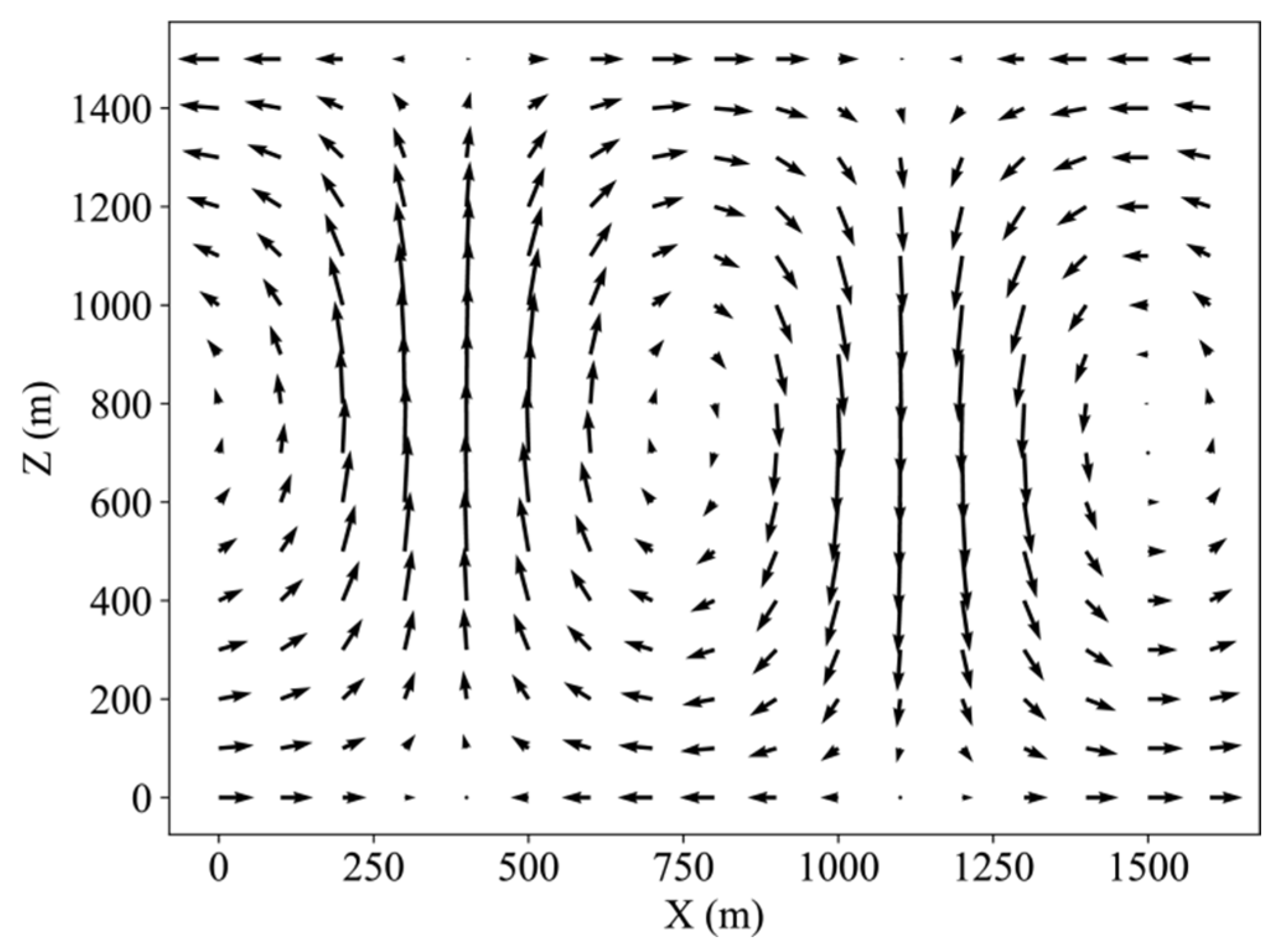
2.1. Initial Field Setup

During the precipitation process, the transport of substances such as water vapor and liquid water in the air is primarily guided by wind vectors, with materials transported along the direction of the wind. The Arabas model constructs an idealized convective scenario and greatly simplifies the dynamic processes. It employs a stream function to calculate the initial background wind field, which is used to simulate the formation of precipitation. In the design of our model, this experiment draws inspiration from the approach of the Arabas model. The Arabas model, an open-source C++ model, is hosted on GitHub (Software name: libcloudph++, Version: 1.0, see https://github.com/igfuw/libcloudphxx/wiki, accessed on 25 March 2025). It is encapsulated within the PySDM (Version: 2.0) Python library and named after its author, becoming known as the ‘Arabas model’.

The model employs a stream function to represent the two-dimensional wind field. The experiment assumes that the density of dry air (ρ_d) remains constant over time.

$$\left\{\begin{array}{c}{\rho }_d·u=-{\displaystyle \frac{\partial \mathsf{\psi }}{\partial z}}\\ {\rho }_d·w=-{\displaystyle \frac{\partial \mathsf{\psi }}{\partial x}}\end{array}\right.$$

(1)

Here, ψ = ψ(x, z, t) represents a stream function, where u and w denote the horizontal and vertical components of the wind vector, respectively. The stream function ψ is defined as [26]

$$\mathsf{\psi }(x,z)=-w_{max}·{\displaystyle \frac{X}{\pi }}·sin\left(\pi ·{\displaystyle \frac{z}{Z}}\right)·cos\left(2\pi ·{\displaystyle \frac{x}{X}}\right)$$

(2)

Here, w_max = 0.6 m/s, based on the setup conditions of the Arabas model, the simulation domain has a width of X = 1500 m width and a height of Z = 1500 m height. The coordinates x and z denote positions of different grid points, x ∈ [0, X], z ∈ [0, Z]. The resulting velocity field describes a vortex field containing both updrafts and downdrafts, as illustrated in Figure 1.

In the Arabas model, the authors employ the liquid water potential temperature (denoted as θ_l) as the indicator for initial temperature setting. All grid points at different heights are initialized with a uniform θ_l = 289 K as the initial temperature. The expression for liquid water potential temperature is given by

$${\theta }_l=T·{\left({\displaystyle \frac{p_0}{p}}\right)}^{{\displaystyle \frac{0.285}{1-0.00366·(T-273.15)}}}$$

(3)

Here, p₀ = 1000 hPa, where p denotes the atmospheric pressure at different grid points, and T represents the air temperature. Air density follows the principle of atmospheric hydrostatic equilibrium, with a surface pressure of 1015 hPa. The grid spacing is set at dx = 20 m and dz = 20 m. Initial water vapor content at all grid points is uniformly set to q_v = 7.5 g/kg.

In this paper, the parameter selection, such as the maximum wind speed, grid spacing, and others, adheres to the conditions set by the Arabas model. This approach is taken because the Arabas model employs fixed configurations in terms of the regional scope, grid point resolution, and the height of vertical layers, which are not readily adjustable during model operation. Consequently, we have configured the parameters of this study in accordance with these presets of the Arabas model to ensure the comparability of the research findings.

2.2. Data Description and Model Specification

The model employed in this study utilizes an idealized virtual scenario, thus representing a fictional region. The wind field, temperature, humidity, and pressure conditions involved in the experiment are all set according to the preceding hypothetical conditions.

This paper discusses the Arabas model, whose code is hosted on GitHub (access address: https://github.com/igfuw/libcloudphxx/wiki, accessed on 25 March 2025). The model employs a unique architecture where particle swarms carry physical quantities such as water vapor. In this model, particles persist on their trajectories. In contrast, the diagnostic model used in this study adopts a gridded approach, storing physical quantities like water vapor and liquid water in regular grid cells, thus forming a grid-based simulation system. The distinction between this grid model and the particle model lies in its focus on the spatial discretization of physical quantities, enabling a detailed simulation of atmospheric processes.

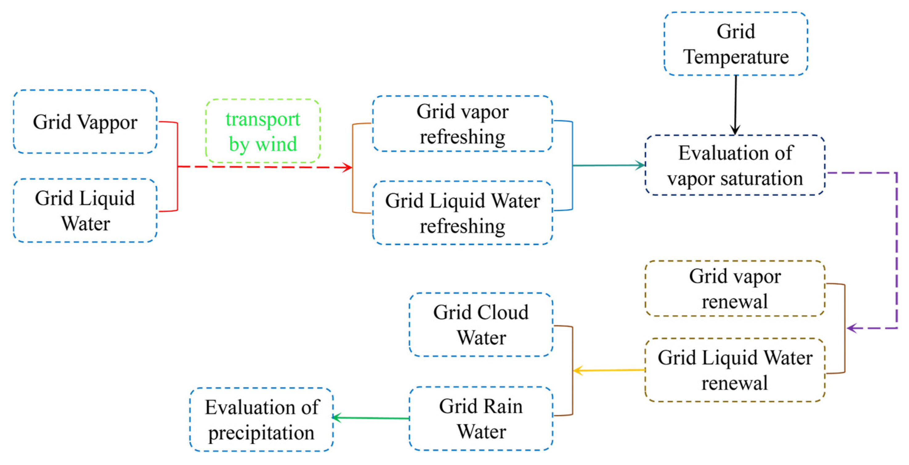
2.3. Water Vapor Condensation

The moisture content in the air is limited; once saturated, water vapor condenses onto aerosols to form liquid droplets. The determination of vapor saturation employs the Clausius–Clapeyron equation, initially calculating the water vapor pressure in the air [27]:

$$es=611.2·e^{{\displaystyle \frac{17.67·T_c}{T_c+243.5}}}$$

(4)

Here, es denotes the vapor pressure generated by water vapor in the air, measured in Pascals (Pa), and T_c represents the air temperature in degrees Celsius, where T_c = T − 273.15.

The specific humidity at saturation corresponding to temperature T_c is calculated as [28]

$$q_{sat}=0.622·{\displaystyle \frac{es}{p-es}}$$

(5)

Here, q_sat represents the threshold of gaseous water that 1 kg of air can hold, measured in kg/kg. When the moisture content in the air exceeds this threshold, the excess condenses into liquid water. In practical modeling, a relative humidity threshold is set at RH = 1.05, assuming that when the water vapor content surpasses 1.05·q_sat, the program determines that the excess water vapor condenses into liquid form.

Within the computational framework of this model, separate arrays are designated for storing the variables of “gaseous water” and “liquid water”. When the model’s algorithm detects that the water vapor content at a specific grid point meets the condensation criteria, the amount of water vapor exceeding the condensation threshold is deducted from the “gaseous water” array. This excess water vapor is then converted into “liquid water” and added to the corresponding position in the “liquid water” array. This mechanism ensures the accurate simulation of the water vapor condensation process within the model.

2.4. Material Transport

In calculating the transport of water vapor and liquid water in the atmosphere, the material transport equation is typically employed [29]:

$${\displaystyle \frac{\partial m}{\partial t}}+u{\displaystyle \frac{\partial m}{\partial x}}+w{\displaystyle \frac{\partial m}{\partial z}}=\kappa ·{\nabla }^2\left(m\right)+S$$

(6)

Here, m denotes substances such as water vapor and liquid water, κ represents the diffusion coefficient, and S denotes the source term.

The model employs the finite difference method to solve partial differential equations, approximating the time partial derivative as follows [30]:

$${\displaystyle \frac{\partial m}{\partial t}}\approx {\displaystyle \frac{m_i^{n+1}-m_i^n}{∆t}}$$

(7)

Approximations for the first-order partial derivative are [31]

$${\displaystyle \frac{\partial m}{\partial x}}\approx {\displaystyle \frac{m_{i+1}^n-m_{i-1}^n}{2·∆x}}$$

(8)

Approximations for the second-order partial derivative are [32]

$${\displaystyle \frac{{\partial }^{2}m}{\partial x^2}}\approx {\displaystyle \frac{m_{i+1,j}-2m_{i,j}+m_{i-1,j}}{∆x^2}}$$

(9)

The material transport equation is formulated using the above approach. Following the same computational principles, this operational method is also applicable to the differentiation operations in the vertical direction (z-direction).

2.5. Temperature Equation

For two-dimensional scenarios, the temperature convection–diffusion equation assumes the following form:

$${\displaystyle \frac{\partial T}{\partial t}}+u·{\displaystyle \frac{\partial T}{\partial x}}+v·{\displaystyle \frac{\partial T}{\partial z}}=\alpha ·\left({\displaystyle \frac{{\partial }^{2}T}{\partial x^2}}+{\displaystyle \frac{{\partial }^{2}T}{\partial z^2}}\right)$$

(10)

It is essential to account for the variation in temperature in relation to altitude [33,34]:

$$c_p{\displaystyle \frac{dT}{dt}}=-gw-L_v·{\displaystyle \frac{dq}{dt}}$$

(11)

Here, c_p denotes the specific heat capacity of air, with c_p = 1005 J/(kg·K), and L_v represents the latent heat of water vapor, which is 2260 kJ/kg at standard atmospheric pressure. Generally, c_p remains constant, while L_v exhibits minor fluctuations with temperature changes. In the equation, dq/dt represents the heat absorbed or released during water vapor phase change. w denotes vertical velocity, and g represents gravity.

In the equation above, −gw accounts for temperature variations due to the static equilibrium process. When calculating temperature diffusion across different vertical grid points in the model, adjustments are made to exclude temperature changes caused by the static equilibrium process.

As shown in Figure 2, the flowchart depicts the experimental design of a precipitation diagnostic model. This diagram outlines the computational process from the transport of water vapor and liquid water in the air to their condensation.

In the actual atmosphere, liquid water in the air exists not in isolation but adheres to aerosol particles, forming water droplets. Generally, small water droplets are referred to as ‘cloud droplets’ and larger ones as ‘raindrops’. In the real atmosphere, when there are enough cloud droplets present, they collide and merge to form raindrops. Due to the uneven size distribution of cloud and raindrop particles, precipitation models often need to establish particle spectra to describe the distribution characteristics of particles within cloud and raindrop formations. This particle spectrum model is also known as a ‘cloud microphysics’ model.

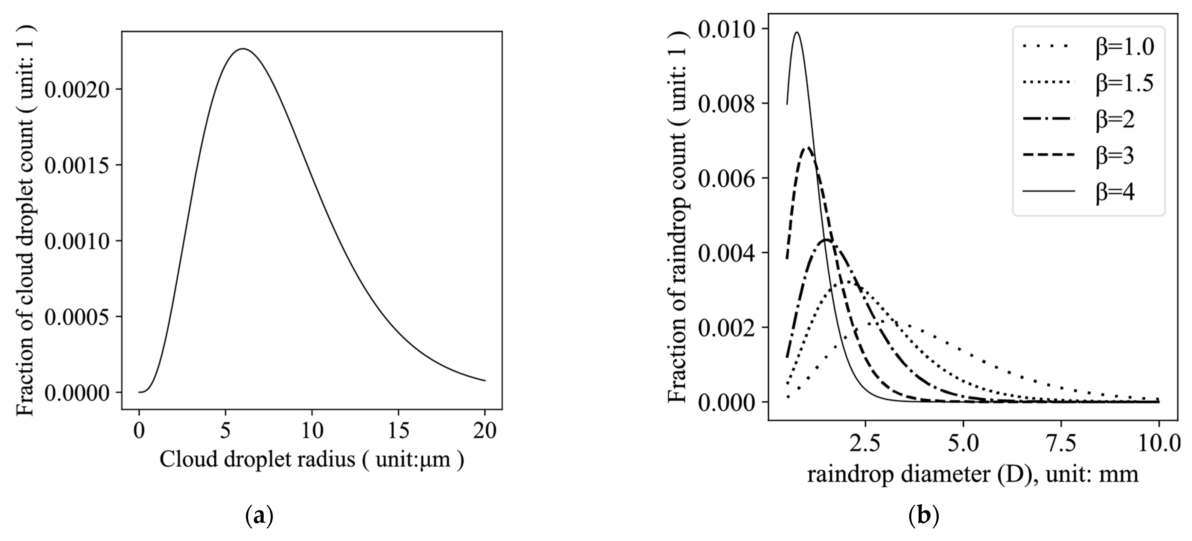
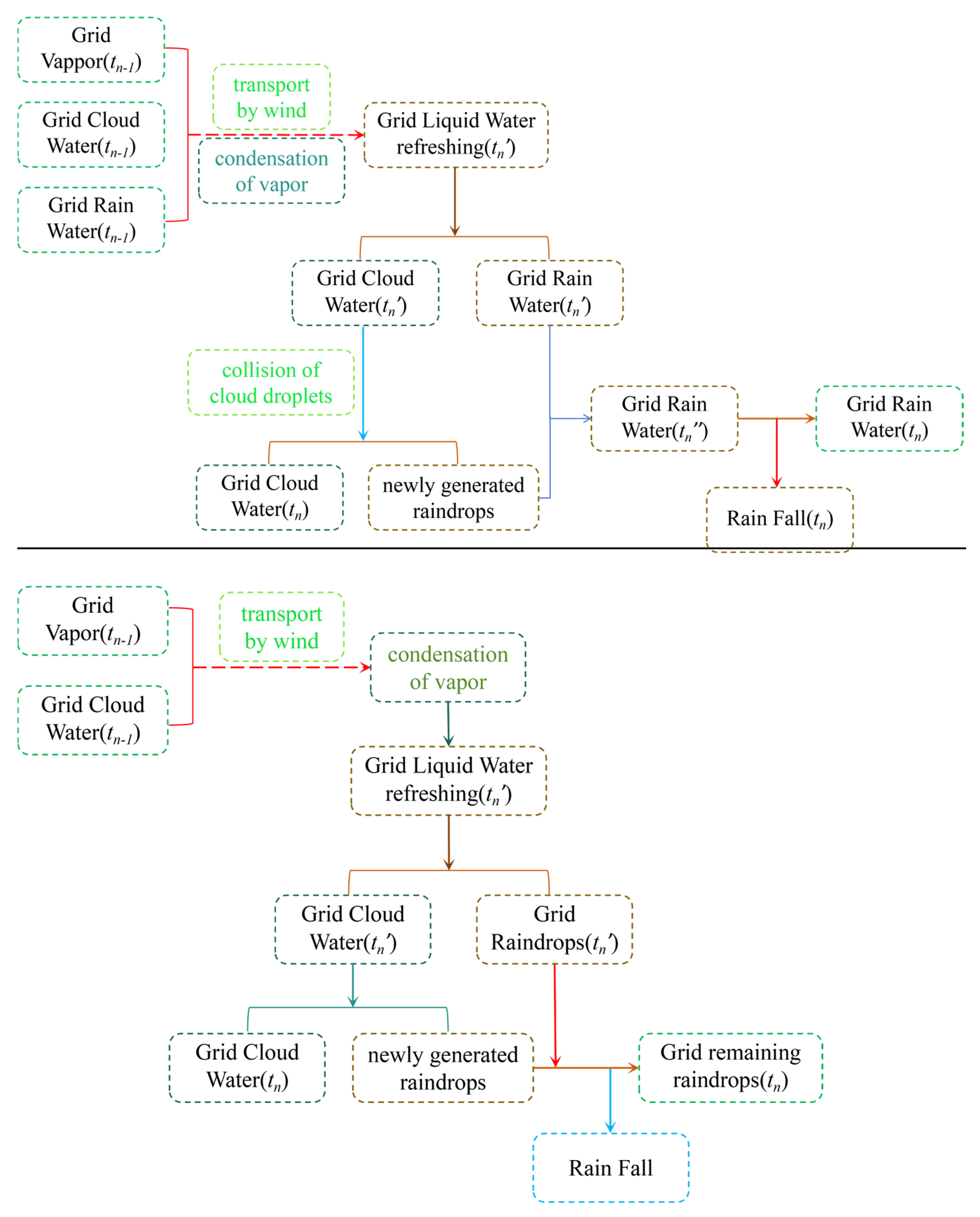
3. Design of the Precipitation Model

The previous section described the construction of a water vapor condensation model within a dynamic framework. This section presents the design approach for the precipitation model.

In the Arabas model, the authors assumed cloud droplet sizes follow a lognormal distribution [35], and they outlined the algorithm for cloud droplet aggregation leading to raindrop formation [36]. This chapter primarily focuses on the design of the precipitation scheme for the diagnostic model [37].

The “diagnostic model” adopts a double-moment framework, which involves establishing two sets of forecast equations with distinct parameters for two different types of particles: cloud droplets and raindrops. Spectral function models utilize the mathematical equations of Gamma distributions to establish relationships between droplet size and particle counts.

Axel Seifert et al. [38] proposed that the cloud droplet spectrum can be expressed using the Gamma function:

$$\left\{\begin{array}{c}{f}_c\left(t\right)=A·t^{\mu }·e^{-Bt}\\ x=R_0·t \end{array},tϵ(\mathrm{0,10}]\right.$$

(12)

In the above equation, the parameter t serves as the independent variable, x represents particle radius, and f_c denotes the cloud droplet distribution spectrum. Here, A, B, and μ are adjustable parameters, with μ set to 3 for this experiment (μ can be 0, 1, 2, or 3), and parameters A = 1, B = 1. The equation includes R₀ = 20 × 10^–7 m and x_max = 20 × 10^–6 m, indicating a maximum cloud droplet size of 20 μm.

Similarly, the raindrop spectrum can be expressed using the Gamma function:

$$f_r\left(D\right)=\alpha ·D^{\mu }{e}^{-\beta D}$$

(13)

Here, D represents the raindrop diameter, with values ranging from 0.04 to 1 mm. Parameters α and β are adjustable parameters that can be chosen based on empirical data; for this experiment, μ is set to 3.

As shown in Figure 3, characteristic distribution functions are constructed for cloud droplet and raindrop spectra, displaying the proportion of particles of different sizes within their respective populations. According to Figure 3b, the parameter β for the raindrop spectrum needs to be selected judiciously.

A dynamic mapping between liquid water content and the parameter β, with β ∈ [1, 4], is incorporated into the model’s parameterization design. The parameter β takes on different values corresponding to the varying levels of liquid water content: it reaches a maximum of 4 when the liquid water content is minimal and decreases to a minimum of 1 as the liquid water content increases. This approach aids the model in more effectively capturing the trends in raindrop mass distribution.

Assuming both cloud and raindrop particles are spherical, the formula for calculating particle volume is

$$V(r)={\displaystyle \frac{3}{4}}·\pi ·r^3$$

(14)

The formula for calculating the mass of cloud and raindrop particles is

$$m\left(r\right)=\rho V\left(r\right)$$

(15)

Here, ρ represents the density of water, and m(r) denotes the density of water. Using the above equations, the mass of cloud and raindrop particles of different diameters can be calculated. Assuming N_c and N_r represent the total number of particles in the cloud and raindrop spectra, respectively, according to Equations (15) and (16), we calculate the total mass of liquid water corresponding to the cloud spectrum (m_cloud) and the raindrop spectrum (m_rain).

$$m_{cloud}={\int }_0^{r_{max}}m\left(r\right)·f_c$$

(16)

$$m_{rain}={\int }_0^{\infty }m\left(r\right)·f_r$$

(17)

The number of particles N_c and N_r in the cloud and raindrop spectra correspond to the total mass of liquid water m_cloud and m_rain, respectively, determining the actual number of particles in the cloud (N_c) and rain (N_r) spectra per unit mass (1 g) of liquid water. This allows us to ascertain the number of cloud droplets (N_c) and raindrops (N_r) corresponding to different masses of liquid water.

Typically, after water vapor condenses in the air, it initially exists in the form of cloud droplets [39]. Subsequently, cloud droplets gradually aggregate to form raindrops. In precipitation models, after water vapor condensation, it first forms cloud droplets, and algorithms are established to simulate the aggregation of cloud droplets into raindrops for calculating raindrop mass [40]. Extensive research has been conducted in this area [41,42,43], and this work utilizes a reduced-form equation for calculating the conversion rate [44]:

$$\tau =1-{\displaystyle \frac{q_r}{q_c+q_r}}$$

(18)

$$P_{au}=\left\{\begin{array}{c}0,{ q}_v\le q_{sat}\\ k·\tau ·\left(q_c-q_{c_0}\right), q_v>q_{sat}\end{array}\right.$$

(19)

Here, q_c and q_r represent the water content of cloud droplets and raindrops, respectively. P_au represents the conversion rate of cloud droplets to raindrops, with units of g/(kg·s). This formula facilitates the condensation process of cloud droplets into raindrops. When a sufficient amount of liquid water has aggregated into raindrops, exceeding thresholds in both size and mass, precipitation is deemed to occur.

As shown in Figure 4, the iterative process of the precipitation diagnostic procedure is presented. First, at the time t_n−1, water vapor and liquid water (including cloud droplets and raindrops) are transported along the wind direction to the grid. The saturation of each grid point is then calculated, and based on the saturation, the liquid water content is reassessed, updating the grid’s liquid water content. This moment is denoted as t_n′ (t_n′ representing a time between t_n−1 and t_n). Next, based on the ratio of cloud droplet to raindrop content at t_n−1, the liquid water at time t_n′ is divided into cloud droplets and raindrops. Using an empirical formula for cloud droplet aggregation into raindrops, the cloud droplet and raindrop contents are updated, yielding the raindrop content at time t_n′. When the mass of large raindrops exceeds a certain threshold, precipitation is identified. After accounting for the fallen raindrops, the raindrop content at time t_n is determined.

In summary, the model is built upon the water vapor and liquid water transport model, incorporating a water vapor condensation determination algorithm, and develops a relatively simple rainfall prediction model. The design of this model draws inspiration from the libcloudph model [45] proposed by Arabas (referred to as the Arabas model in this paper).

4. Results

4.1. Model Calculation Results

In accordance with the configuration of the Arabas model, which involves a spin-up phase of at least 45 min prior to operation (with this approach, water vapor is able to spread and flow sufficiently, which optimizes its distribution across the atmosphere), this study utilizes the diagnostic model in two distinct approaches to simulate weather conditions after 30 min: (a) the Diagnostic Normal scheme, which does not include a spin-up phase, and (b) the Diagnostic Spin-Up scheme, which incorporates a 45-min pre-computed spin-up phase during which no precipitation processes are activated.

As illustrated in Figure 5, the results of the model simulation after 30 min indicate that all four scenarios predict cloud formation at approximately 1 km above ground level. A distinct “gap” in the cloud layer is observed near x = 1.15 km, which is attributed to the presence of descending airflows in this region. As the air descends, it is compressed and heated due to increased environmental pressure, causing cloud droplets to evaporate into water vapor and resulting in the observed “gap” in the cloud layer. In contrast, at x = 0.2 to 0.5 km, the cloud water content is higher. The diagnostic model suggests that the droplets in this region may have dispersed from the convective center, indicating that the upward air movements in this area have facilitated the vertical transport and condensation of water vapor, thereby increasing the liquid water concentration in the cloud layer.

In precipitation models, high-altitude liquid water is divided into cloud droplets and raindrops. As water vapor condenses, it initially forms cloud droplets, which coalesce to create clouds. When cloud water content becomes sufficient, cloud droplets collide and merge to form larger raindrops. This process remains a challenge in precipitation research, with significant differences observed in outcomes across various cloud microphysics models.

As shown in Figure 6, after 30 min of simulation, the results for the rain water mixing ratio in the air from the four schemes exhibit significant differences. The diagnostic model (Figure 6a,b) calculations indicate that the cloud layers containing large raindrops are thicker, whereas the Arabas model (Figure 6c,d) shows that the overall thickness of the cloud layers containing large raindrops is thinner. Although both the single-moment scheme (Figure 6c) and double-moment bulk scheme (Figure 6d) of the Arabas model are theoretically consistent in terms of the dynamical framework and water vapor transport, the considerable differences in the simulation results underscore the uncertainty inherent in cloud microphysics modeling.

As illustrated in Figure 6a,b, the simulation results from the two diagnostic model schemes show that the regions with a higher content of large raindrops are located above the vicinity of the coordinate x = 1.15 km. Similarly, as shown in Figure 6d, a considerable aggregation of raindrops is observed above the coordinate x = 1.15 km. It can be seen from the figures that the areas of high raindrop concentration in Figure 6a,b,d are consistent. The main difference between Figure 6a,b,d is that the overall cloud layer thickness in Figure 6a,b is greater than that in Figure 6d. As shown in Figure 6d, this scheme is able to simulate the raindrop aggregation effect in the airflow convergence region, while the raindrop aggregation effect is not significant in the updraft region.

Figure 7 illustrates the results of water vapor content (vapor mixing ratio) in the air after 30 min of simulation across three schemes. It can be observed that, driven by the vortex airflow, in Figure 7a, there is a pronounced accumulation of water vapor above the convergence center of the airflow (at x = 0.3 km). In the downdraft region (at x = 1.1 km), the water vapor is pushed towards the lower atmosphere due to the impact of the dry airflow from above. In Figure 7b, the situation is similar to that in Figure 7a, with the distinction that the vortex’s promotional effect results in a more pronounced distribution of the airflow. The water vapor transport process in the Arabas model (Figure 7c) is relatively gentle, with changes in water vapor content observed only at the center of the downdraft region during the sinking of the upper-airflow. These results indicate that the diagnostic model is more sensitive in simulating water vapor transport and distribution, capturing complex atmospheric dynamic processes more effectively.

Figure 8 reveals the pronounced vertical variation characteristics of water vapor content distribution across different altitude levels. Figure 8a depicts the distribution of water vapor content in the updraft region, whereas Figure 8b illustrates the situation in the downdraft region. In detail, Figure 8a shows that at higher altitudes (above 0.9 km), the water vapor content significantly decreases with increasing height. Both the diagnostic model and the Arabas model demonstrate high consistency in this vertical gradient change, although there are some differences in the details. These discrepancies may arise from the different treatments of water vapor transport mechanisms and cloud microphysical processes in the two models. In the lower-altitude region near the surface (below 0.9 km), the Arabas model predicts a roughly stable water vapor content of around 7.5 g/kg, whereas the diagnostic model exhibits slight fluctuations in water vapor content due to the convergence effect of the airflow. This result indicates that different models show varying responses to airflow dynamics when simulating near-surface water vapor content, offering a new perspective for understanding the complexity of atmospheric water vapor distribution.

In Figure 8b, in comparing the simulation results between the diagnostic model and the Arabas model, we have identified certain discrepancies. Specifically, the output from the diagnostic model reveals a continuous decreasing trend in water vapor content with decreasing altitude. In contrast, the simulation results from the Arabas model exhibit a unique “arched” distribution, where the water vapor content reaches a peak in the mid-to-high altitude range (between 0.6 and 0.9 km) at approximately 7.3 g/kg. At higher altitudes and in the lower atmospheric regions, the water vapor content decreases, but the magnitude of the decrease is relatively small.

Figure 9 presents the statistical information of spatial precipitation from the diagnostic model and the Arabas model (double-moment bulk scheme) over a 30-min period, revealing the spatial characteristics of precipitation distribution. Figure 9a–c illustrate the mass of raindrops falling from the upper atmosphere and the spatial distribution of precipitation triggering, while Figure 9d provides statistical data on total precipitation at the ground level. The precipitation region of the diagnostic model is primarily concentrated around x = 0.3 km, where upward air currents lead to increased precipitation amounts, indicating that this area is conducive to convective rainfall. In contrast, around x = 1.25 km, the precipitation amount is lower due to the influence of sinking air currents, suggesting that these currents help suppress rainfall occurrence. The precipitation patterns from the Arabas model (double-moment bulk scheme) show certain commonalities with those of the diagnostic model, yet differ in some aspects. The predominant precipitation zone is located around x = 1.25 km. This phenomenon is primarily attributed to the collision and coalescence processes of raindrops. After the spin-up process, the precipitation results from the diagnostic model show subtle changes, with an overall increasing trend In precipitation amounts.

4.2. Model Computational Efficiency

To evaluate the computational speed of the model, this study measured the computation time using a Xeon E5 2650 processor (Device source: China, Wuhan, Huazhong University of Science and Technology, Digital Water Resources Laboratory). The model was implemented in Python utilizing the Cupy library for GPU parallel computing. Iteration time steps and their corresponding execution times were recorded, with a time step δt set to 15 s. The total duration of the simulation was 30 min, requiring 120 time steps.

From

Table 1. Iteration count and time consumption.

Time Consumption	Number of Iteration Time Steps
11.8 s	10
24.5 s	20
40.3 s	40
79.4 s	80
108.5 s	120

, it can be observed that the model consumes an average of approximately 1 s per time step. Considering the model’s implementation in Python, there is still room for improvement in computational efficiency.

Based on testing, the Arabas model requires approximately 25 min to simulate a 30-min scenario. This extended time is primarily attributed to the model’s use of Lagrangian particle tracking for material transport, which heavily taxes CPU resources. Additionally, the complex algorithms in the cloud microphysics scheme further contribute to computational demands. Moreover, the Arabas model operates on a single-core CPU, limiting computational speed. In contrast, the diagnostic model efficiently leverages Python’s GPU acceleration libraries, significantly speeding up calculations.

5. Discussion

The construction of precipitation models is inherently complex, involving intricate interactions among dynamic processes, moisture condensation, and microphysical processes. These complexities pose significant challenges in understanding and researching the precipitation mechanism. To simplify modeling and enhance comprehension of the intermediate processes, this study innovatively adopts a stream function approach to replace traditional dynamic models. By simulating atmospheric flow through a simplified vorticity field and incorporating a precipitation diagnostic model, we evaluate the effectiveness of precipitation simulations. This approach provides valuable insights for future research and improvements in precipitation algorithms.

In the simulation of convective precipitation, it is evident that with current technological means, relying on meteorological Doppler radar, laser wind measuring equipment, and combining wind field inversion simulations, researchers are able to relatively accurately invert the wind fields within thunderstorm systems. Therefore, it can be considered that wind field data within thunderstorm systems can be obtained through actual measurements.

Given the three-dimensional wind field characteristics of a thunderstorm system, the question arises of how to design diagnostic models for precipitation that simulate the physical processes of water vapor transport, phase transition of water vapor, and weather evolution, in order to calculate the formation process of convective weather. This research is of great value and significance for improving precipitation simulation and advancing the development of small-scale meteorological numerical models. To date, there remains a substantial amount of work to be completed in this field. The aforementioned research necessitates integrating atmospheric dynamic processes, water vapor transport, phase changes in water vapor, and the triggering and formation of precipitation, which presents certain challenges and requires the continuous development of technical methods.

In the future, the construction of precipitation models requires further optimization and design refinement. For instance, the stream function approach utilized in this experiment could be enhanced or replaced using machine learning models. Similarly, cloud microphysics models can benefit from optimization and improvement through machine learning techniques. Additionally, integrating real-time information from weather radars and other sources is essential to enhance the simulation accuracy of precipitation models in urban areas, high mountain regions, and valleys.

6. Conclusions

This study constructs a two-dimensional z-x sectional precipitation model, which simulates the lifting and condensation of water vapor under a simple background wind field, while integrating a precipitation diagnostic scheme. Driven by the vortex wind field, the model effectively simulates the transport, ascent, and descent of water vapor and liquid water, and observes the distribution patterns of the resulting precipitation. After evaluating the simulation’s performance, the following conclusions are drawn:

(I)

In this study, we constructed a hypothetical vortex wind field model to simulate the transport and phase transitions of water vapor and liquid water, achieving efficient computation while effectively replicating the associated physical processes. Moving forward, we aim to utilize radar inversion technology to obtain actual wind field data, which will serve as the model’s driving force to investigate the accuracy of precipitation simulation under true wind conditions. This approach will offer critical technical support for assessing and refining precipitation models, enhancing the reliability and utility of the simulation outcomes.

(II)

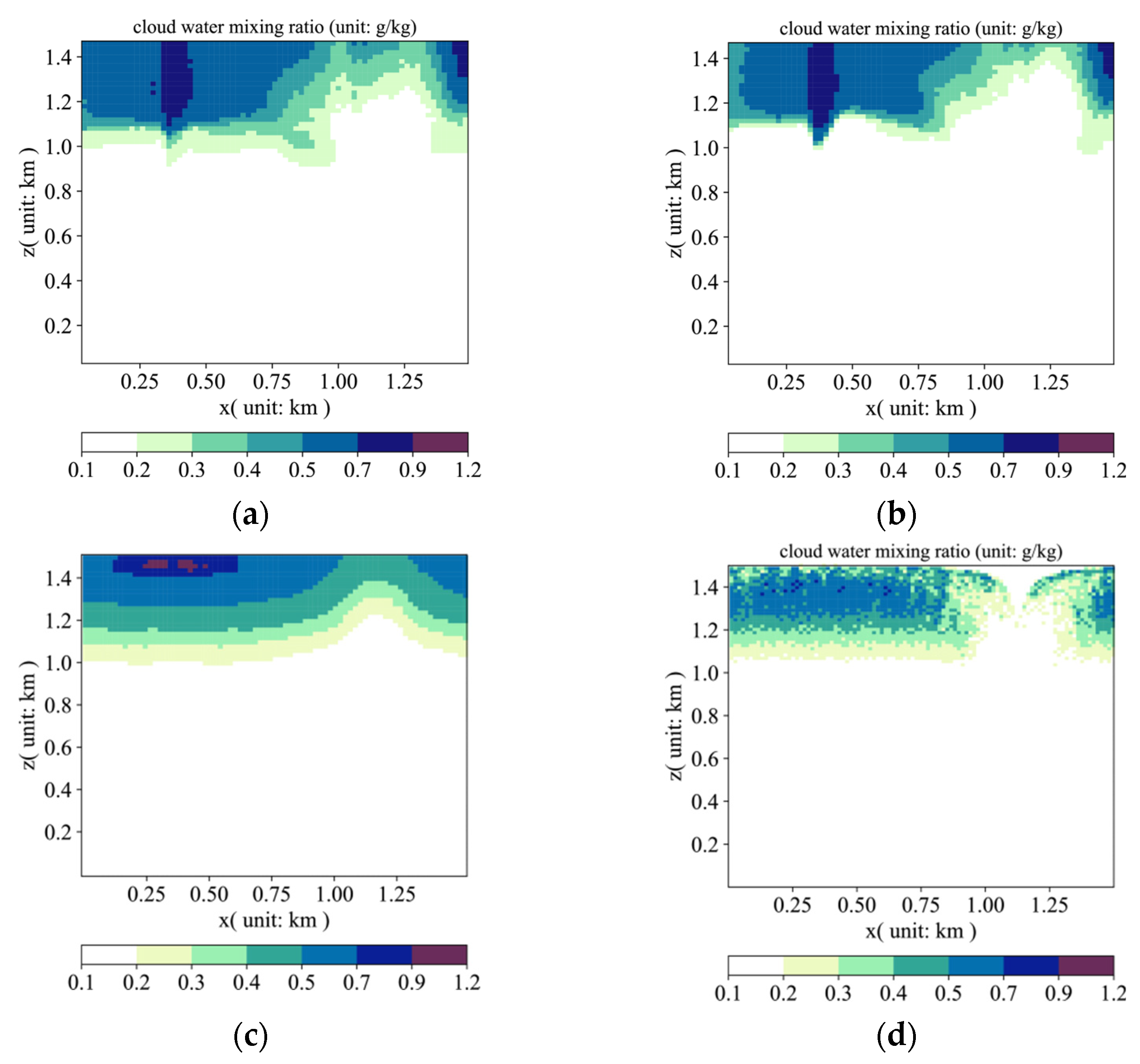
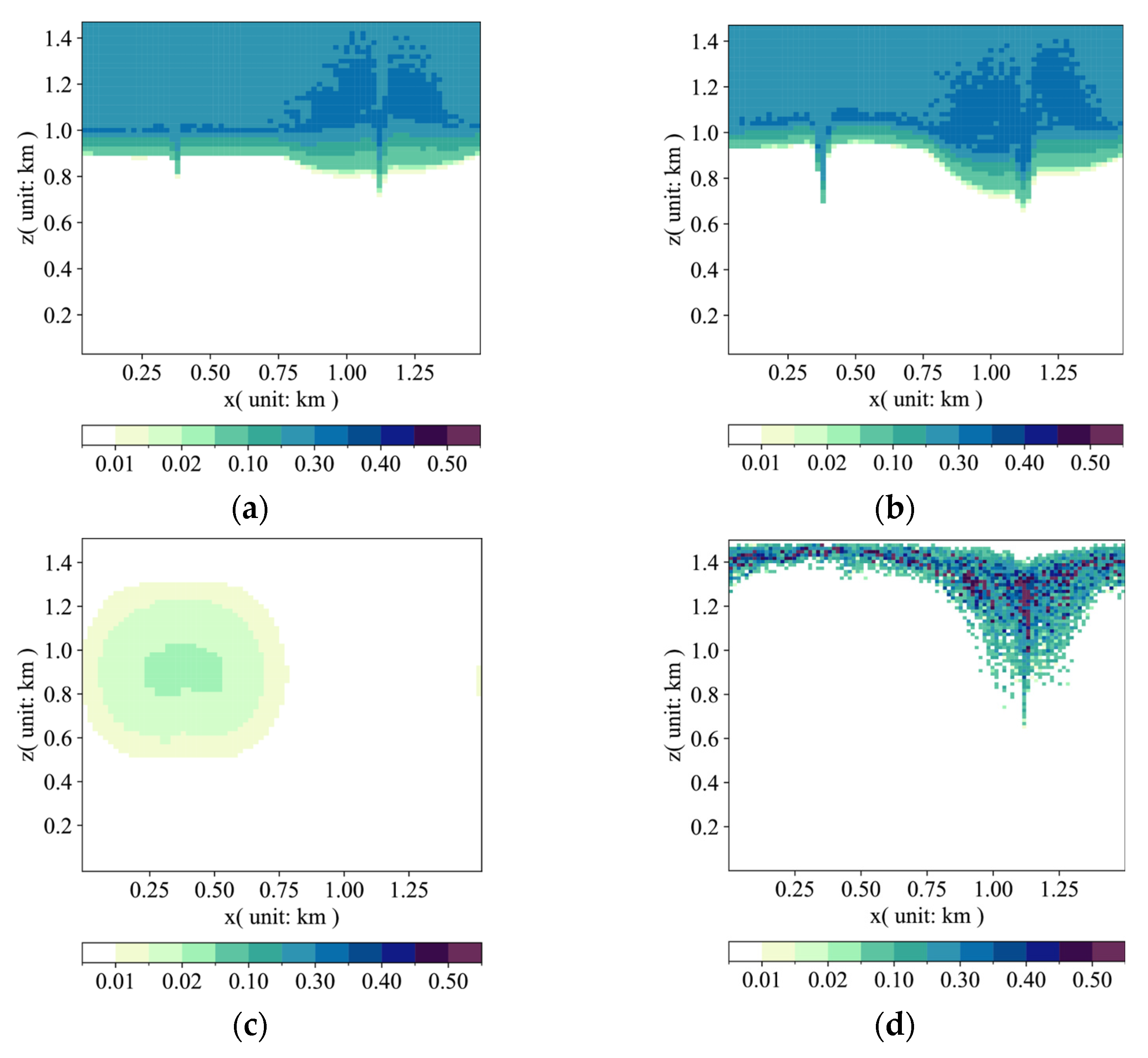
This study developed a diagnostic model that comprehensively simulates the water vapor condensation process, taking into account the controlling influence of atmospheric temperature and pressure. The model precisely captures the decreasing threshold of saturated vapor content as altitude rises and temperature drops. As lower-level water vapor is lifted to higher atmospheric layers, it condenses into liquid water, leading to cloud formation. Our model not only replicates the condensation process but also reveals stratification with increasing height, offering a robust tool for understanding precipitation formation dynamics.

(III)

Simulating precipitation is a multifaceted and complex process influenced by atmospheric dynamics, water vapor transport, and condensation lift, and is constrained by the chosen precipitation algorithms. Accurate representation of the precipitation formation process is crucial for computational outcomes. Nevertheless, due to the complexity of precipitation mechanisms and limitations in experimental data acquisition, our understanding of precipitation simulation remains incomplete and uncertain.

This study’s model provides a robust tool for understanding and predicting precipitation distribution. Despite challenges in simulating cloud microphysical processes, the model’s overall performance underscores its potential in precipitation simulation.

References

1. Guo, J.; Xu, X.J.; Lian, W.W.; Zhu, H.L. A new approach for interval forecasting of photovoltaic power based on generalized weather classification. Int. Trans. Electr. Energy Syst. 2019, 29, e2802. [Google Scholar] [CrossRef]
2. Guo, J.; Liu, Y.; Zou, Q.; Ye, L.; Zhu, S.; Zhang, H. Study on optimization and combination strategy of multiple daily runoff prediction models coupled with physical mechanism and LSTM. J. Hydrol. 2023, 624, 129969. [Google Scholar]
3. Chang, X.; Guo, J.; Qin, H.; Huang, J.; Wang, X.; Ren, P. Single-Objective and Multi-Objective Flood Interval Forecasting Considering Interval Fitting Coefficients. Water Resour. Manag. 2024, 38, 3953–3972. [Google Scholar] [CrossRef]
4. Turner, R.; McConney, P.; Monnereau, I. Climate Change Adaptation and Extreme Weather in the Small-Scale Fisheries of Dominica. Coast. Manag. 2020, 48, 436–455. [Google Scholar] [CrossRef]
5. Zhang, S.; Solari, G.; De Gaetano, P.; Burlando, M.; Repetto, M.P. A refined analysis of thunderstorm outflow characteristics relevant to the wind loading of structures. Probabil. Eng. Mech. 2017, 54, 9–24. [Google Scholar] [CrossRef]
6. Kurowski, M.J.; Wojcik, D.K.; Ziemianski, M.Z.; Rosa, B.; Piotrowski, Z.P. Convection-permitting regional weather modeling with COSMO-EULAG: Compressible and anelastic solutions for a typical westerly flow over the Alps. Mon. Weather Rev. 2016, 144, 1961–1982. [Google Scholar] [CrossRef]
7. Garcia-Dorado, I.; Aliaga, D.G.; Bhalachandran, S.; Schmid, P.; Niyogi, D. Fast Weather Simulation for Inverse Procedural Design of 3D Urban Models. ACM Trans. Graph. 2017, 36, 21. [Google Scholar]
8. Wei, X.; Liu, Y.; Guo, J.; Chang, X.; Li, H. Applicability Study of Euler–Lagrange Integration Scheme in Constructing Small-Scale Atmospheric Dynamics Models. Atmosphere 2024, 15, 644. [Google Scholar] [CrossRef]
9. Makarieva, A.M.; Gorshkov, V.G.; Nefiodov, A.V.; Sheil, D.; Nobre, A.D.; Bunyard, P.; Nobre, P.; Li, B. The equations of motion for moist atmospheric air. J. Geophys. Res. Atmos. 2017, 122, 7300–7307. [Google Scholar] [CrossRef]
10. Oreskovic, C.; Savory, E.; Porto, J.; Orf, L.G. Evolution and scaling of a simulated downburst-producing thunderstorm outflow. Wind. Struct. 2018, 26, 147–161. [Google Scholar]
11. Zhou, Y.; Li, X. An Analysis of Thermally-Related Surface Rainfall Budgets Associated with Convective and Stratiform Rainfall. Adv. Atmos. Sci. 2011, 28, 1099–1108. [Google Scholar]
12. Engin, L.; Gokhan, A.; Tuncer, I.H. Wind potential estimations based on unsteady turbulent flow solutions coupled with a mesoscale weather prediction model. In Proceedings of the 7th Ankara International Aerospace Conference, Ankara, Turkey, 11–13 September 2013. [Google Scholar]
13. Wei, X.; Liu, Y.; Chang, X.; Guo, J.; Li, H. Numerical Simulation of Terrain-Adaptive Wind Field Model Under Complex Terrain Conditions. Water 2024, 16, 2138. [Google Scholar] [CrossRef]
14. Choi, H.W.; Kim, D.Y.; Kim, J.J.; Kim, K.Y.; Woo, J.H. Study on Dispersion Characteristics for Fire Scenarios in an Urban Area Using a CFD-WRF Coupled Model. Atmosphere 2012, 22, 47–55. [Google Scholar] [CrossRef]
15. Miao, J.-E.; Yang, M.-J. A Modeling Study of the Severe Afternoon Thunderstorm Event at Taipei on 14 June 2015: The Roles of Sea Breeze, Microphysics, and Terrain. J. Meteorol. Soc. Jpn. 2020, 98, 129–152. [Google Scholar]
16. Groot, E.; Tost, H. Analysis of variability in divergence and turn-over induced by three idealized convective systems with a 3D cloud resolving model. Atmos. Chem. Phys. 2020, 2020, 1–23. [Google Scholar] [CrossRef]
17. Guo, Z.; Zhao, J.; Zhao, P.; He, M.; Yang, Z.; Su, D. Simulation Study of Microphysical and Electrical Processes of a Thunderstorm in Sichuan Basin. Atmosphere 2023, 14, 574. [Google Scholar] [CrossRef]
18. Pu, Z.; Lin, C.; Dong, X.; Krueger, S.K. Sensitivity of Numerical Simulations of a Mesoscale Convective System to Ice Hydrometeors in Bulk Microphysical Parameterization. Pure Appl. Geophys. 2019, 176, 2097–2120. [Google Scholar] [CrossRef]
19. Poulsen, T.; Niclasen, B.A.; Giebel, G.; Beyer, H.G. Validation of WRF generated wind field in complex terrain. Meteorol. Z. 2021, 30, 413–428. [Google Scholar] [CrossRef]
20. Noh, I.; Lee, S.-J.; Lee, S.; Kim, S.-J.; Yang, S.-D. A High-Resolution (20 m) Simulation of Nighttime Low Temperature Inducing Agricultural Crop Damage with the WRF–LES Modeling System. Atmosphere 2021, 12, 1562. [Google Scholar] [CrossRef]
21. Putnam, B.J.; Xue, M.; Jung, Y.; Zhang, G.; Kong, F. Simulation of Polarimetric Radar Variables from 2013 CAPS Spring Experiment Storm-Scale Ensemble Forecasts and Evaluation of Microphysics Schemes. Mon. Weather Rev. 2017, 145, 49–73. [Google Scholar]
22. Martynova, Y.V.; Zaripov, R.B.; Krupchatnikov, V.N.; Petrov, A.P. Estimation of the quality of atmospheric dynamics forecasting in the siberian region using the wrf-arw mesoscale model. Russ. Meteorol. Hydrol. 2014, 39, 440–447. [Google Scholar] [CrossRef]
23. Xue, H.; Li, J.; Zhang, Q.; Gu, H. Simulation of the Effect of Small-Scale Mountains on Weather Conditions During the May 2021 Ultramarathon in Gansu Province, China. J. Geophys. Res. Atmos. JGR 2022, 127, e2022JD036465. [Google Scholar]
24. Arabas, S.; Jaruga, A.; Pawlowska, H.; Grabowski, W.W. libcloudph++ 0.2: Single-moment bulk, double-moment bulk, and particle-based Diagnostic microphysics library in C++. Geosci. Model. Dev. Discuss. 2014, 7, 8275–8360. [Google Scholar]
25. Morrison, H.; Grabowski, W.W. Comparison of Bulk and Bin Warm-Rain Microphysics Models Using a Kinematic Framework. J. Atmos. Sci. 2006, 64, 2839–2861. [Google Scholar]
26. Rasinski, P.; Pawlowska, H.; Grabowski, W.W. Observations and kinematic modeling of drizzling marine stratocumulus. Atmos. Res. 2011, 102, 120–135. [Google Scholar] [CrossRef]
27. Bolton, D. The Computation of Equivalent Potential Temperature. Mon. Weather Rev. 1980, 108, 1046–1053. [Google Scholar]
28. Schneider, T.; O′Gorman, P.A.; Levine, X.J. Water vapor and the dynamics of climate change. Rev. Geophys. 2010, 48, RG3001. [Google Scholar] [CrossRef]
29. Grell, G.A.; Dudhia, J.; Stauffer, D.R. A Description of the Fifth-Generation Penn State/NCAR Mesoscale Model (MM5); Technical Report NCAR/TN-398+STR; National Center for Atmospheric Research: Boulder, CO, USA, 1994. [Google Scholar]
30. Cullen, M.J.P.; Davies, T. A conservative split-explicit integration scheme with fourth-order horizontal advection. Q. J. R. Meteorol. Soc. 1991, 117, 993–1002. [Google Scholar]
31. Leslie, L.M.; Purser, R.J. High-Order Numerics in an Unstaggered Three-Dimensional Time-Split Semi-Lagrangian Forecast Model. Mon. Weather Rev. 2009, 119, 1612–1623. [Google Scholar] [CrossRef]
32. Tremback, C.J.; Powell, J.; Cotton, W.R.; Pielke, R.A. The Forward–in-Time Upstream Advection Scheme: Extension to Higher Orders. Mon. Weather Rev. 1987, 115, 540–555. [Google Scholar] [CrossRef]
33. Rothenberg, D.; Wang, C. Metamodeling of Droplet Activation for Global Climate Models. J. Atmos. Sci. 2016, 73, 1255–1272. [Google Scholar] [CrossRef]
34. Yang, F.; Kollias, P.; Shaw, R.A.; Vogelmann, A.M. Cloud droplet size distribution broadening during diffusional growth: Ripening amplified by deactivation and reactivation. Atmos. Chem. Phys. 2018, 18, 7313–7328. [Google Scholar] [CrossRef]
35. Jaruga, A.; Pawlowska, H. libcloudph++2.0: Aqueous-phase chemistry extension of the particle-based cloud microphysics scheme. Geosci. Model Dev. 2018, 11, 3623–3645. [Google Scholar] [CrossRef]
36. Allen, G.; Coe, H.; Clarke, A.; Bretherton, C.; Wood, R.; Abel, S.J.; Barrett, P.; Brown, P.; George, R.; Freitag, S.; et al. South East Pacific atmospheric composition and variability sampled along 20 degrees S during VOCALS-REx. Atmos. Chem. Phys. 2011, 11, 5237–5262. [Google Scholar] [CrossRef]
37. Nober, F.J.; Graf, H.F. A new convective cloud field model based on principles of self-organisation. Atmos. Chem. Phys. 2004, 4, 3669–3698. [Google Scholar] [CrossRef]
38. Seifert, A.; Beheng, K.D. A double-moment parameterization for simulating autoconversion, accretion and selfcollection. Atmos. Res. 2001, 59, 265–281. [Google Scholar] [CrossRef]
39. Bott, A. A flux method for the numerical solution of the stochastic collection equation. J. Atmos. Sci. 1998, 55, 2284–2293. [Google Scholar] [CrossRef]
40. Lebo, Z.J.; Seinfeld, J.H. A continuous spectral aerosol-droplet microphysics model. Atmos. Chem. Phys. Discuss. 2011, 11, 23655–23705. [Google Scholar] [CrossRef]
41. Chiu, J.C.; Yang, C.K.; Jan van Leeuwen, P.; Feingold, G.; Wood, R.; Blanchard, Y.; Mei, F.; Wang, J. Observational Constraints on Warm Cloud Microphysical Processes Using Machine Learning and Optimization Techniques. Geophys. Res. Lett. 2021, 48, e2020GL091236. [Google Scholar] [CrossRef]
42. Axel, S.; Stephan, R. Potential and Limitations of Machine Learning for Modeling Diagnostic Cloud Microphysical Processes. J. Adv. Model. Earth Syst. 2020, 12, e2020MS002301. [Google Scholar]
43. Khairoutdinov, M.; Kogan, Y. A new cloud physics parameterization in a large-eddy simulation model of marine stratocumulus. Mon. Weather Rev. 2000, 128, 229–243. [Google Scholar]
44. Berry, E.X. Modification of the warm rain process. National Conference on Weather Modification. Amer. Meteor. Soc. 1968, 49, 154. [Google Scholar]
45. Sylwester, A.; Shin-ichiro, S. On the CCN (de) activation nonlinearities. Nonlinear Process. Geophys. 2017, 24, 535–542. [Google Scholar]
Figure 1. Schematic of vortex wind field.
Atmosphere 16 00380 g001
Figure 2. Flowchart for precipitation diagnosis.
Atmosphere 16 00380 g002
Figure 3. The characteristics of particle spectrum distribution. The horizontal axis represents the size of water droplets, while the vertical axis shows the proportion of particles of different sizes. (a) displays the cloud droplet spectrum distribution characteristics; (b) shows the raindrop spectrum distribution characteristics, where changes in β values alter the features of the spectrum.
Atmosphere 16 00380 g003
Figure 4. Iterative calculation of cloud microphysical processes. Here, tn represents the time at the n-th timestep, tn′ represents a time between tn−1 and tn, and tn′ ’ represents a time between tn′ and tn.
Atmosphere 16 00380 g004
Figure 5. Contour plots of cloud water mixing ratio (unit: g/kg) in the atmosphere simulated after 30 min. (a) Results from the Diagnostic Model Normal scheme; (b) Results from the Diagnostic Model Spin-Up scheme; (c) Results from the Arabas model with single-moment bulk scheme; (d) Results from the Arabas model with double-moment bulk scheme.
Atmosphere 16 00380 g005
Figure 6. Contour plots of rain water mixing ratio (unit: g/kg) in the atmosphere simulated after 30 min. (a,b) results from diagnotic model; (c) results from the Arabas model with single-moment bulk scheme: (d) Results from the Arabas model with double-moment bulk scheme.
Atmosphere 16 00380 g006
Figure 7. Contour plots of vapor mixing ratio (unit: g/kg) in the atmosphere simulated after 30 min. (a) Results from the Diagnostic Model Normal scheme; (b) Results from the Diagnostic Model Spin-Up scheme; (c) Results from the Arabas model with double-moment bulk scheme.
Atmosphere 16 00380 g007
Figure 8. Distribution of water vapor at different altitude levels. The horizontal axis represents specific humidity (g/kg), while the vertical axis denotes altitude. This includes results from the Diagnostic Model Normal, Diagnostic Model Spin-Up, and Arabas (double-moment bulk scheme) models. (a) Average results for updraft conditions. (b) Average results for descending air conditions.
Atmosphere 16 00380 g008
Figure 9. Distribution of rainfall mass triggered within 30 min. Unit: mm. (a) Rainfall triggered above the diagnostic model; (b) Rainfall triggered above the spin-up scheme of the diagnostic model; (c) Rainfall triggered above the Arabas model (double-moment bulk scheme); (d) Spatial distribution of rainfall amounts across the three schemes within 30 min.
Atmosphere 16 00380 g009