
Artificial Neural Network for Air Pollutant Concentration Predictions Based on Aircraft Trajectories over Suvarnabhumi International Airport

 ,
, 
 ,
,  ,
,  and
and 
Abstract
1. Introduction
2. Related
2.1. K-Means
2.2. Gaussian Mixture Model
2.3. Silhouette Score
2.4. Evaluation Metrics
3. Materials and Methods
3.1. Pollution Emission Data
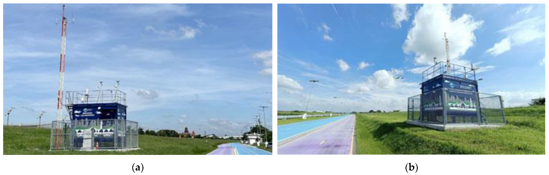
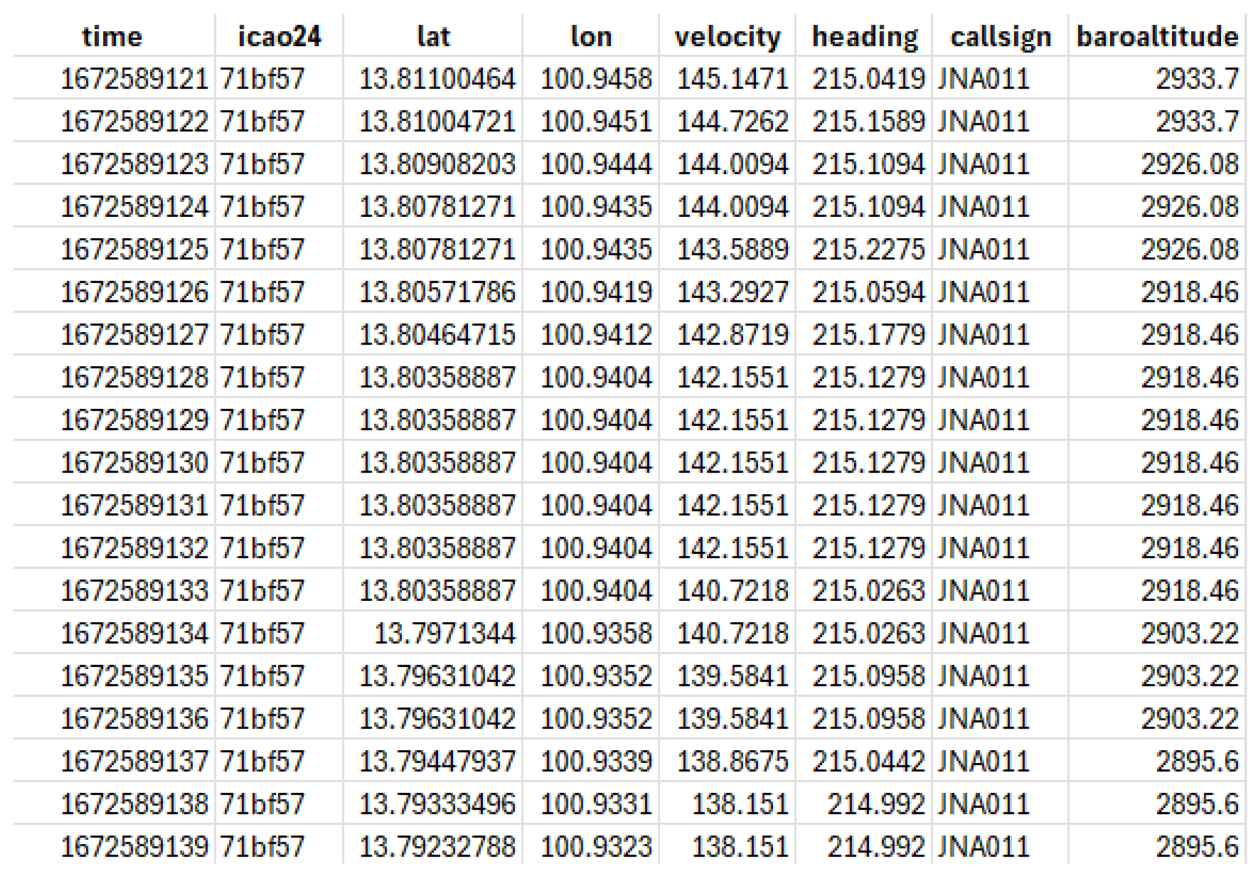
3.2. Trajectory Data
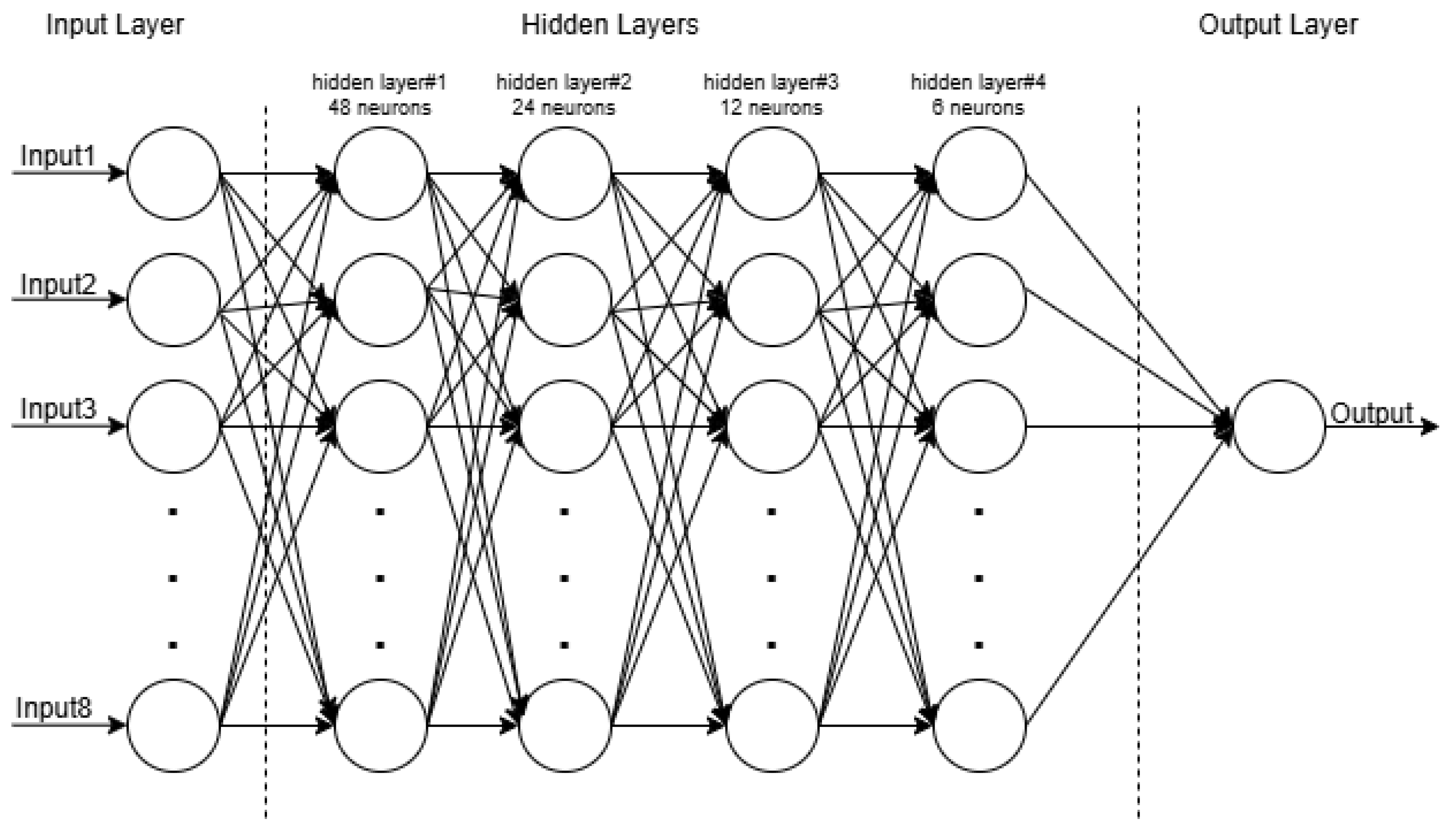
3.3. Methods
4. Results
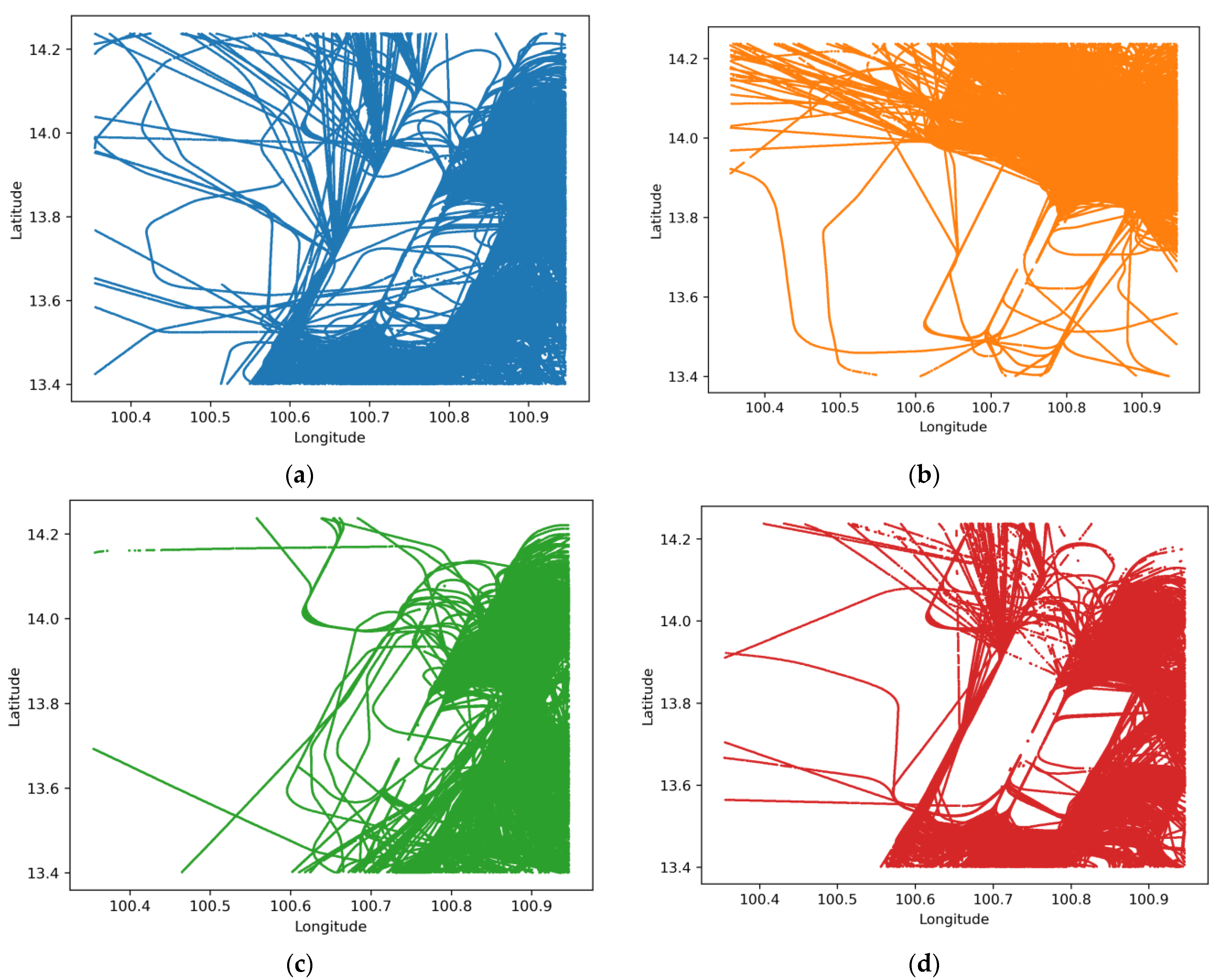
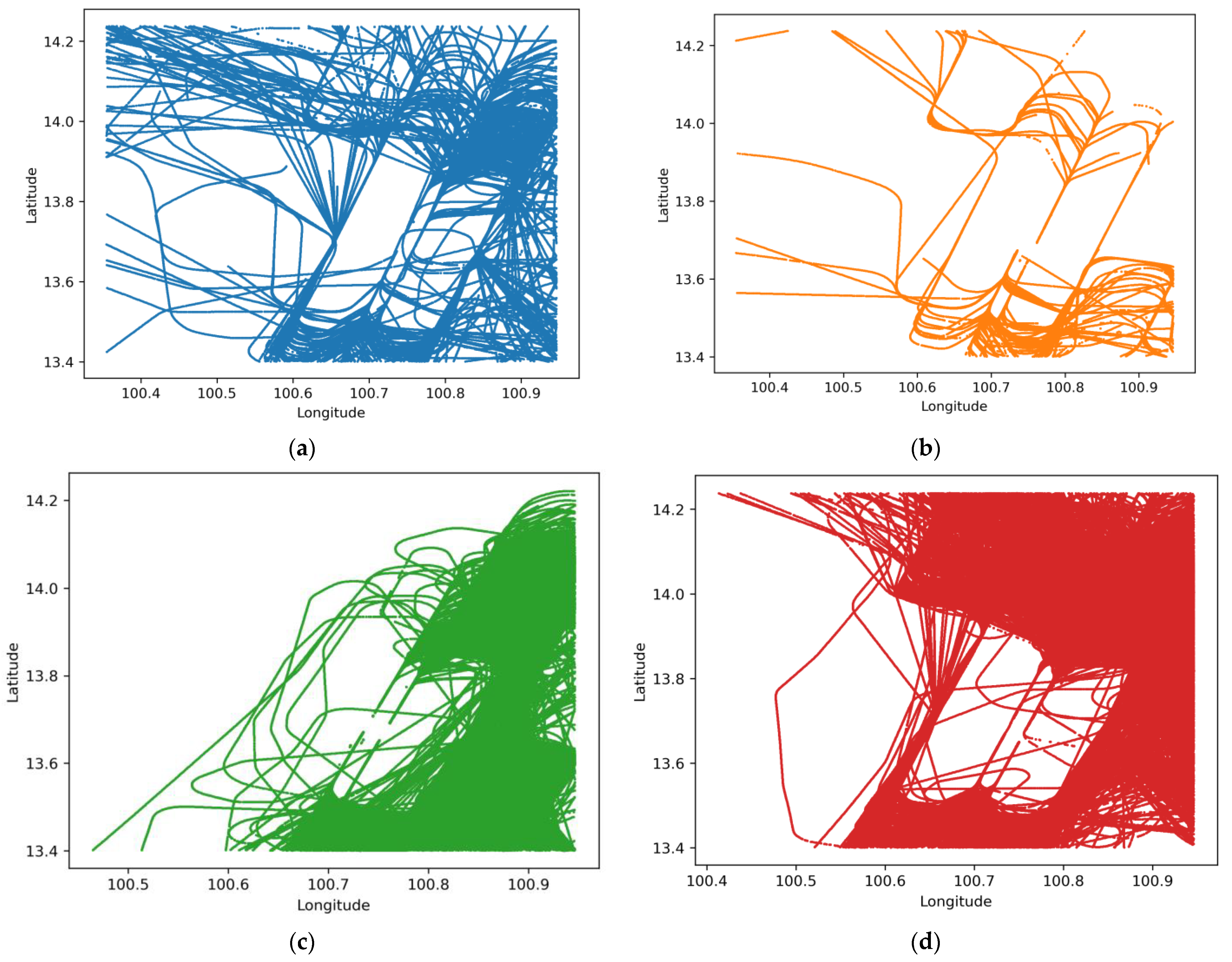
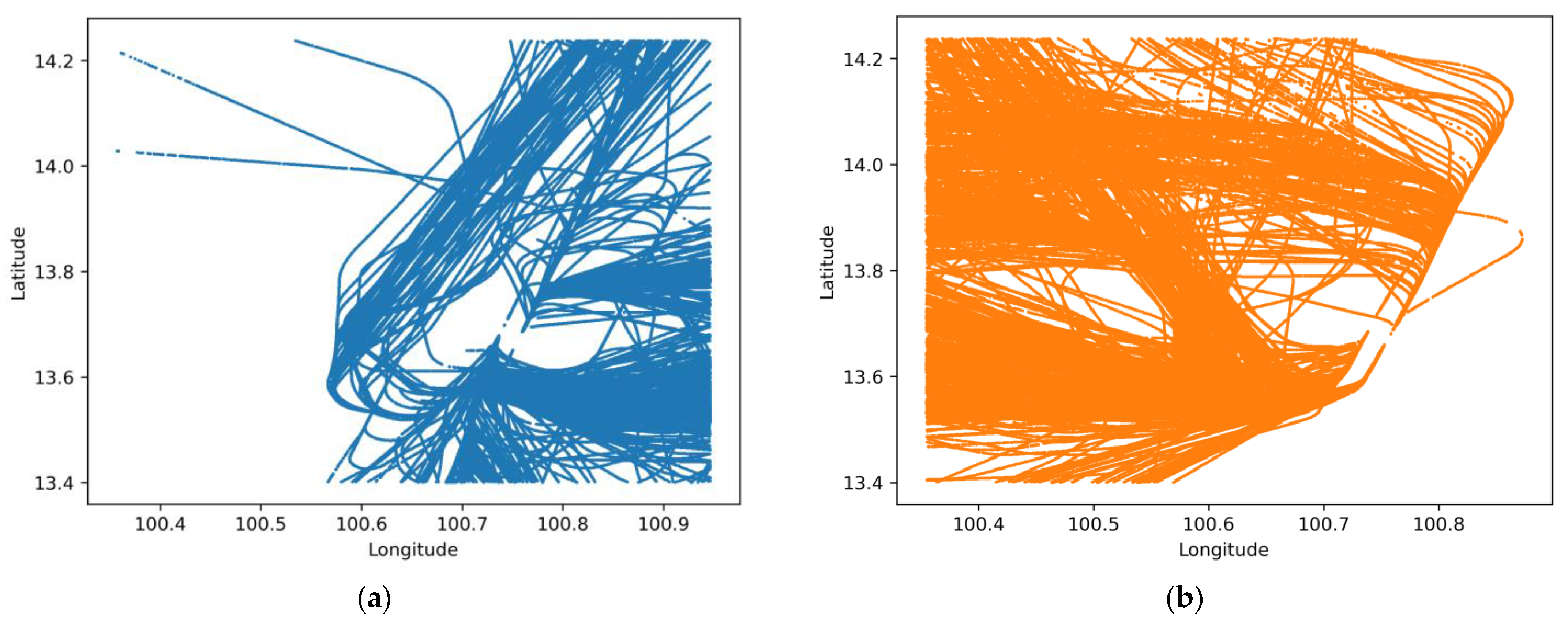
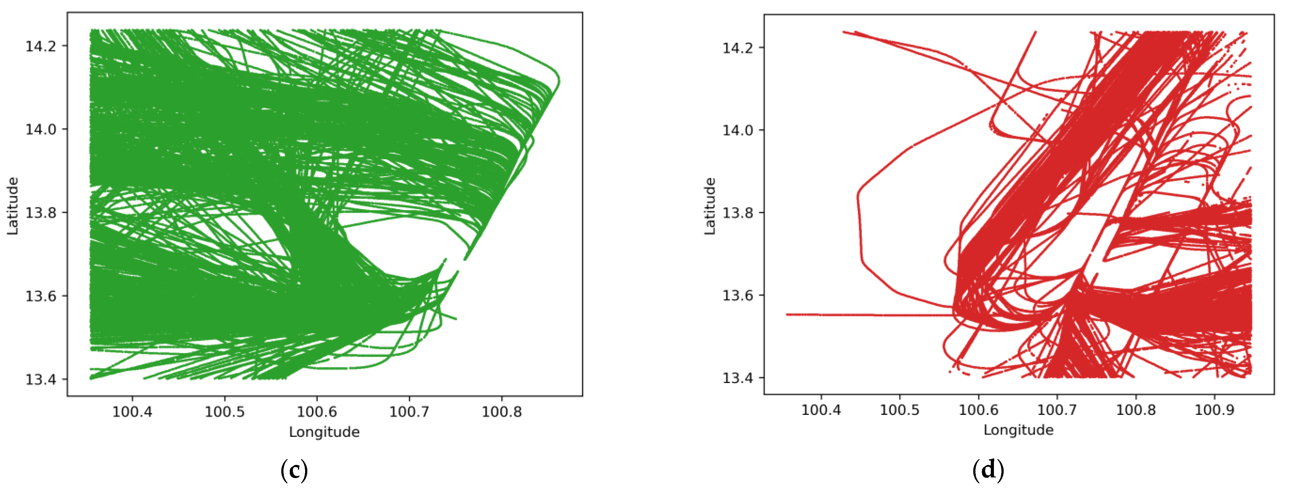
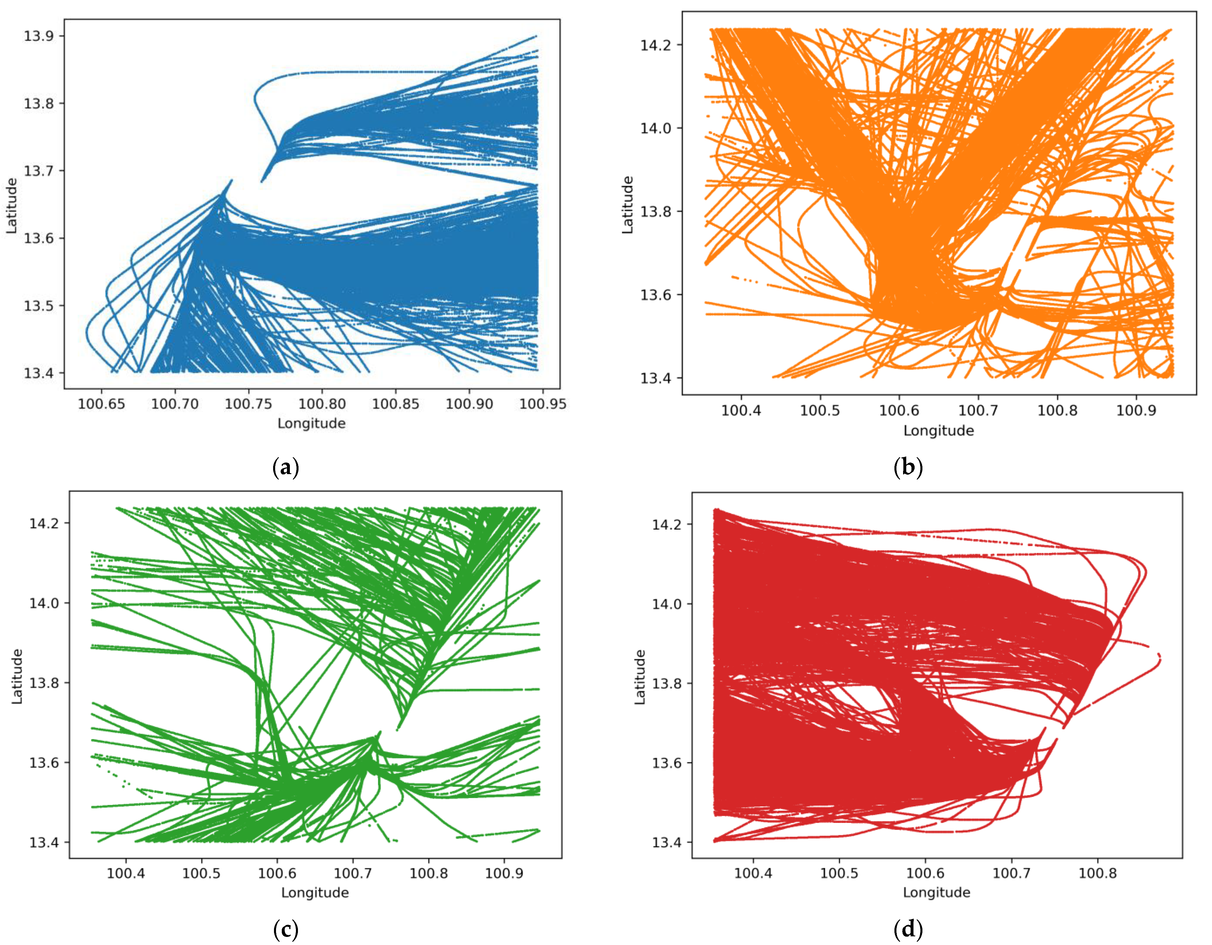
4.1. K-Means and GMM Clustering Results
4.2. Regression Model Results
5. Conclusions
Author Contributions
Funding
Institutional Review Board Statement
Informed Consent Statement
Data Availability Statement
Acknowledgments
Conflicts of Interest
Appendix A
References
- Airports of Thailand Public Co., Ltd. Air Transport Statistic. Available online: https://investor.airportthai.co.th/transport.html (accessed on 24 January 2025).
- Tian, Y.; Wan, L.; Ye, B.; Yin, R.; Xing, D. Optimization Method for Reducing the Air Pollutant Emission and Aviation Noise of Arrival in Terminal Area. Sustainability 2019, 11, 4715. [Google Scholar] [CrossRef]
- Xu, X.; Dong, D.; Wang, Y.; Wang, S. The Impacts of Different Air Pollutants on Domestic and Inbound Tourism in China. Int. J. Environ. Res. Public Health 2019, 16, 5127. [Google Scholar]
- Zeng, W.; Xu, Z.; Cai, Z.; Chu, X.; Lu, X. Aircraft Trajectory Clustering in Terminal Airspace Based on Deep Autoencoder and Gaussian Mixture Model. Aerospace 2021, 8, 266. [Google Scholar] [CrossRef]
- Wang, Z.-S.; Zhang, Z.-Y.; Cui, Z. Research on Resampling and Clustering Method of Aircraft Flight Trajectory. J. Signal Process. Syst. 2023, 95, 319–331. [Google Scholar] [CrossRef]
- Kamsing, P.; Torteeka, P.; Yooyen, S.; Yenpiem, S.; Delahaye, D.; Notry, P.; Phisannupawong, T.; Channumsin, S. Aircraft Trajectory Recognition Via Statistical Analysis Clustering for Suvarnabhumi International Airport. In Proceedings of the 2020 22nd International Conference on Advanced Communication Technology (ICACT), Phoenix Park, Republic of Korea, 16–19 February 2020; pp. 290–297. [Google Scholar]
- Adams-Selin, R.D. A Three-Dimensional Hail Trajectory Clustering Technique. Mon. Weather. Rev. 2023, 151, 2361–2375. [Google Scholar] [CrossRef]
- Yin, J.; Zhang, M.; Ma, Y.; Wu, W.; Li, H.; Chen, P. Prediction and Analysis of Airport Surface Taxi Time: Classification, Features, and Methodology. Appl. Sci. 2024, 14, 1306. [Google Scholar] [CrossRef]
- Yadav, V.; Yadav, A.K.; Singh, V.; Singh, T. Artificial Neural Network an Innovative Approach in Air Pollutant Prediction for Environmental Applications: A Review. Results Eng. 2024, 22, 102305. [Google Scholar] [CrossRef]
- Jairi, I.; Ben-Othman, S.; Canivet, L.; Zgaya-Biau, H. Enhancing Air Pollution Prediction: A Neural Transfer Learning Approach across Different Air Pollutants. Environ. Technol. Innov. 2024, 36, 103793. [Google Scholar] [CrossRef]
- Cordova, C.H.; Portocarrero, M.N.L.; Salas, R.; Torres, R.; Rodrigues, P.C.; López-Gonzales, J.L. Air Quality Assessment and Pollution Forecasting Using Artificial Neural Networks in Metropolitan Lima-Peru. Sci. Rep. 2021, 11, 24232. [Google Scholar] [CrossRef]
- Rahman, P.A.; Panchenko, A.A.; Safarov, A.M. Using Neural Networks for Prediction of Air Pollution Index in Industrial City. IOP Conf. Ser. Earth Environ. Sci. 2017, 87, 042016. [Google Scholar] [CrossRef]
- Djebbri, N.; Rouainia, M. Artificial Neural Networks Based Air Pollution Monitoring in Industrial Sites. In Proceedings of the 2017 International Conference on Engineering and Technology (ICET), Antalya, Turkey, 21–23 August 2017; pp. 1–5. [Google Scholar]
- Araghinejad, S. Data-Driven Modeling: Using MATLAB® in Water Resources and Environmental Engineering; Springer Science & Business Media: Berlin, Germany, 2013. [Google Scholar]
- Leontaritis, I.J.; Billings, S.A. Input-Output Parametric Models for Non-Linear Systems Part I: Deterministic Non-Linear Systems. Int. J. Control 1985, 41, 303–328. [Google Scholar] [CrossRef]
- Simpkins, A. System Identification: Theory for the User, 2nd Edition (Ljung, L.; 1999) [On the Shelf]. IEEE Robot. Autom. Mag. 2012, 19, 95–96. [Google Scholar] [CrossRef]
- Kurt, A.; Gulbagci, B.; Karaca, F.; Alagha, O. An Online Air Pollution Forecasting System Using Neural Networks. Environ. Int. 2008, 34, 592–598. [Google Scholar] [CrossRef]
- Kalajdjieski, J.; Zdravevski, E.; Corizzo, R.; Lameski, P.; Kalajdziski, S.; Pires, I.M.; Garcia, N.M.; Trajkovik, V. Air Pollution Prediction with Multi-Modal Data and Deep Neural Networks. Remote Sens. 2020, 12, 4142. [Google Scholar] [CrossRef]
- Maleki, H.; Sorooshian, A.; Goudarzi, G.; Baboli, Z.; Tahmasebi Birgani, Y.; Rahmati, M. Air Pollution Prediction by Using an Artificial Neural Network Model. Clean Technol. Environ. Policy 2019, 21, 1341–1352. [Google Scholar] [CrossRef] [PubMed]
- Kristiyanti, D.; Purwaningsih, E.; Nurelasari, E.; Hairul Umam, A. Implementation of Neural Network Method for Air Quality Forecasting in Jakarta Region. J. Phys. Conf. Ser. 2020, 1641, 012037. [Google Scholar] [CrossRef]
- Nandi, B.P.; Singh, G.; Jain, A.; Tayal, D.K. Evolution of Neural Network to Deep Learning in Prediction of Air, Water Pollution and Its Indian Context. Int. J. Environ. Sci. Technol. 2024, 21, 1021–1036. [Google Scholar] [CrossRef]
- Li, X.; Peng, L.; Yao, X.; Cui, S.; Hu, Y.; You, C.; Chi, T. Long Short-Term Memory Neural Network for Air Pollutant Concentration Predictions: Method Development and Evaluation. Environ. Pollut. 2017, 231, 997–1004. [Google Scholar] [CrossRef]
- Dong, J.; Goodman, N.; Rajagopalan, P. A Review of Artificial Neural Network Models Applied to Predict Indoor Air Quality in Schools. Int. J. Environ. Res. Public Health 2023, 20, 6441. [Google Scholar] [CrossRef]
- Feng, Q.; Wu, S.; Du, Y.; Huaiping, X.; Xiao, F.; Ban, X.; Li, X. Improving Neural Network Prediction Accuracy for PM10 Individual Air Quality Index Pollution Levels. Environ. Eng. Sci. 2013, 30, 725–732. [Google Scholar] [CrossRef]
- Guo, Q.; He, Z.; Li, S.; Li, X.; Meng, J.; Hou, Z.; Liu, J.; Chen, Y. Air Pollution Forecasting Using Artificial and Wavelet Neural Networks with Meteorological Conditions. Aerosol Air Qual. Res. 2020, 20, 1429–1439. [Google Scholar] [CrossRef]
- Jasiński, R. Analysis of the Applied Flight Trajectory Influence on the Air Pollution in the Area of Warsaw Chopin Airport. J. Ecol. Eng. 2024, 25, 294–305. [Google Scholar] [CrossRef]
- Wang, J.; Zhang, H.; Yu, J.; Lu, F.; Li, Y. Modeling Civil Aviation Emissions with Actual Flight Trajectories and Enhanced Aircraft Performance Model. Atmosphere 2024, 15, 1251. [Google Scholar] [CrossRef]
- Kanungo, T.; Mount, D.M.; Netanyahu, N.S.; Piatko, C.D.; Silverman, R.; Wu, A.Y. An Efficient K-Means Clustering Algorithm: Analysis and Implementation. IEEE Trans. Pattern Anal. Mach. Intell. 2002, 24, 881–892. [Google Scholar]
- Wilkin, G.A.; Huang, X. K-Means Clustering Algorithms: Implementation and Comparison. In Proceedings of the Second International Multi-Symposiums on Computer and Computational Sciences (IMSCCS 2007), Iowa City, IA, USA, 13–15 August 2007. [Google Scholar]
- Qi, J.; Yu, Y.; Wang, L.; Liu, J. K*-Means: An Effective and Efficient K-Means Clustering Algorithm. In Proceedings of the 2016 IEEE International Conferences on Big Data and Cloud Computing (BDCloud), Social Computing and Networking (SocialCom), Sustainable Computing and Communications (SustainCom) (BDCloud-SocialCom-SustainCom), Atlanta, GA, USA, 8–10 October 2016. [Google Scholar]
- Cai, W.; Lei, L.; Yang, M. A Gaussian Mixture Model-Based Clustering Algorithm for Image Segmentation Using Dependable Spatial Constraints. In Proceedings of the 2010 3rd International Congress on Image and Signal Processing, Yantai, China, 16–18 October 2010; pp. 1268–1272. [Google Scholar]
- Li, Y.; Zhang, J.; Ma, Z.; Zhang, Y. Clustering Analysis in the Wireless Propagation Channel with a Variational Gaussian Mixture Model. IEEE Trans. Big Data 2020, 6, 223–232. [Google Scholar] [CrossRef]
- Sun, H.; Liu, Z.; Kong, L. A Document Clustering Method Based on Hierarchical Algorithm with Model Clustering. In Proceedings of the 22nd International Conference on Advanced Information Networking and Applications—Workshops (AINA Workshops 2008), GinoWan, Japan, 25–28 March 2008; pp. 1229–1233. [Google Scholar]
- Zhao, Y.; Shrivastava, A.K.; Tsui, K.L. Regularized Gaussian Mixture Model for High-Dimensional Clustering. IEEE Trans. Cybern. 2019, 49, 3677–3688. [Google Scholar] [CrossRef]
- Rousseeuw, P.J. Silhouettes: A Graphical Aid to the Interpretation and Validation of Cluster Analysis. J. Comput. Appl. Math. 1987, 20, 53–65. [Google Scholar] [CrossRef]
- Airports of Thailand Public Co., Ltd. Online Air Quality Monitoring Report. Available online: https://air4suvarnabhumiairport.com/data.php (accessed on 10 May 2024).
- Mak, H.W.; Ng, D.C. Spatial and Socio-Classification of Traffic Pollutant Emissions and Associated Mortality Rates in High-Density Hong Kong via Improved Data Analytic Approaches. Int. J. Environ. Res. Public Health 2021, 18, 6532. [Google Scholar] [CrossRef]
- Thailand, A. Re-Designation of Runway 01R/19L and 01L/19R at Suvarnabhumi International Airport (VTBS). Available online: https://aip.caat.or.th/2024-10-02/html/eSUP/VT-eSUP-24-41-A-en-GB.html (accessed on 24 January 2025).
- Schäfer, M.; Strohmeier, M.; Lenders, V.; Martinovic, I.; Wilhelm, M. Bringing up Opensky: A Large-Scale Ads-B Sensor Network for Research. In Proceedings of the 13th International Symposium on Information Processing in Sensor Networks, Berlin, Germany, 15–17 April 2014; pp. 83–94. [Google Scholar]
- Federal Aviation Administration. Automatic Dependent Surveillance—Broadcast (ADS-B). Available online: https://www.faa.gov/about/office_org/headquarters_offices/avs/offices/afx/afs/afs400/afs410/ads-b#:~:text=ADS-B%20Out%20works%20by,other%20aircraft%2C%20once%20per%20second (accessed on 24 January 2025).
- Goodfellow, I.; Bengio, Y.; Courville, A. Deep Learning; The MIT Press: Cambridge, MA, USA, 2016. [Google Scholar]
- Xavier, G.; Antoine, B.; Yoshua, B. Deep Sparse Rectifier Neural Networks. In Proceedings of the Fourteenth International Conference on Artificial Intelligence and Statistics, Fort Lauderdale, FL, USA, 11–13 April 2011; pp. 315–323. [Google Scholar]
- Nair, V.; Hinton, G. Rectified Linear Units Improve Restricted Boltzmann Machines Vinod Nair. In Proceedings of the 27th International Conference on Machine Learning (ICML-10), Haifa, Israel, 21–24 June 2010; Volume 27, pp. 807–814. [Google Scholar]
- Mak, H.W.; Laughner, J.L.; Fung, J.C.; Zhu, Q.; Cohen, R.C. Improved Satellite Retrieval of Tropospheric NO2 Column Density via Updating of Air Mass Factor (AMF): Case Study of Southern China. Remote Sens. 2018, 10, 1789. [Google Scholar] [CrossRef]
- Cheng, L.; Tao, J.; Valks, P.; Yu, C.; Liu, S.; Wang, Y.; Xiong, X.; Wang, Z.; Chen, L. NO2 Retrieval from the Environmental Trace Gases Monitoring Instrument (EMI): Preliminary Results and Intercomparison with OMI and TROPOMI. Remote Sens. 2019, 11, 3017. [Google Scholar] [CrossRef]
- Clerbaux, C.; Hadji-Lazaro, J.; Payan, S.; Camy-Peyret, C.; Wang, J.; Edwards, D.P.; Luo, M. Retrieval of Co from Nadir Remote-Sensing Measurements in the Infrared by Use of Four Different Inversion Algorithms. Appl. Opt. 2002, 41, 7068–7078. [Google Scholar] [CrossRef] [PubMed]
- Kamsing, P.; Cao, C.; Zhao, Y.; Boonpook, W.; Tantiparimongkol, L.; Boonsrimuang, P. Joint Iterative Satellite Pose Estimation and Particle Swarm Optimization. Appl. Sci. 2025, 15, 2166. [Google Scholar]
- Fu, D.; Han, S.; Li, W.; Lin, H. The Pose Estimation of the Aircraft on the Airport Surface Based on the Contour Features. IEEE Trans. Aerosp. Electron. Syst. 2023, 59, 817–826. [Google Scholar] [CrossRef]


| Silhouette Score | K1 | K2 | K3 | K4 | |
|---|---|---|---|---|---|
| Landing clustered by K-means | 0.33063 | 1750 | 2303 | 1752 | 1507 |
| Landing clustered by GMM | 0.25064 | 453 | 121 | 2403 | 4335 |
| Take-off clustered by K-means | 0.35264 | 1405 | 1029 | 1004 | 1444 |
| Take-off clustered by GMM | 0.27440 | 2254 | 538 | 570 | 1520 |
| MSE | |
|---|---|
| CO (ppm) | 51.7622 |
| NO2 (ppb) | 139.6674 |
| ) | 53.9682 |
| ) | 124.2517 |
| MAE | MSE | R2 | |
|---|---|---|---|
| CO (ppm) | 2.6373 | 83.7389 | 0.4946 |
| NO2 (ppb) | 9.3116 | 149.8641 | 0.3339 |
| ) | 6.5713 | 70.6187 | 0.4762 |
| ) | 8.3571 | 124.2517 | 0.5594 |
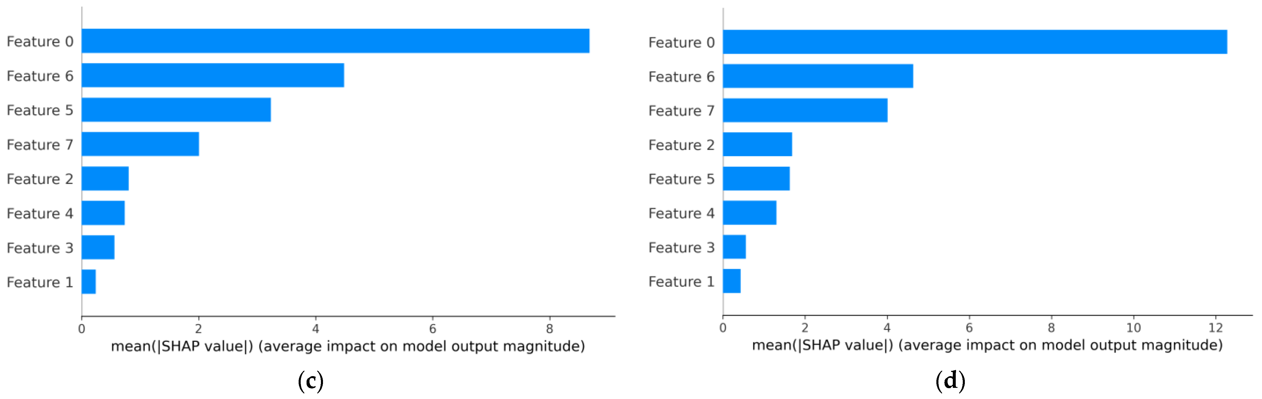
| Feature Number | Representation |
|---|---|
| 0 | Month |
| 1 | Conversion of ICAO24 to integer |
| 2 | Velocity |
| 3 | Heading |
| 4 | Baro altitude |
| 5 | |
| 6 | Pattern numbers that originate from K-means |
| 7 | Pattern numbers that originate from GMM |
Disclaimer/Publisher’s Note: The statements, opinions and data contained in all publications are solely those of the individual author(s) and contributor(s) and not of MDPI and/or the editor(s). MDPI and/or the editor(s) disclaim responsibility for any injury to people or property resulting from any ideas, methods, instructions or products referred to in the content. |
© 2025 by the authors. Licensee MDPI, Basel, Switzerland. This article is an open access article distributed under the terms and conditions of the Creative Commons Attribution (CC BY) license (https://creativecommons.org/licenses/by/4.0/).
Share and Cite
Kamsing, P.; Cao, C.; Boonpook, W.; Boonprong, S.; Xu, M.; Boonsrimuang, P. Artificial Neural Network for Air Pollutant Concentration Predictions Based on Aircraft Trajectories over Suvarnabhumi International Airport. Atmosphere 2025, 16, 366. https://doi.org/10.3390/atmos16040366
Kamsing P, Cao C, Boonpook W, Boonprong S, Xu M, Boonsrimuang P. Artificial Neural Network for Air Pollutant Concentration Predictions Based on Aircraft Trajectories over Suvarnabhumi International Airport. Atmosphere. 2025; 16(4):366. https://doi.org/10.3390/atmos16040366
Chicago/Turabian StyleKamsing, Patcharin, Chunxiang Cao, Wuttichai Boonpook, Sornkitja Boonprong, Min Xu, and Pisit Boonsrimuang. 2025. "Artificial Neural Network for Air Pollutant Concentration Predictions Based on Aircraft Trajectories over Suvarnabhumi International Airport" Atmosphere 16, no. 4: 366. https://doi.org/10.3390/atmos16040366
APA StyleKamsing, P., Cao, C., Boonpook, W., Boonprong, S., Xu, M., & Boonsrimuang, P. (2025). Artificial Neural Network for Air Pollutant Concentration Predictions Based on Aircraft Trajectories over Suvarnabhumi International Airport. Atmosphere, 16(4), 366. https://doi.org/10.3390/atmos16040366