A Case Study of Ozone Pollution in a Typical Yangtze River Delta City During Typhoon: Identifying Precursors, Assessing Health Risks, and Informing Local Governance

Abstract

Ozone (O₃) is a crucial atmospheric component that significantly affects air quality and poses considerable health risks to humans. In the coastal areas of the Yangtze River Delta, typhoons, influenced by the subtropical high-pressure system, can lead to complex ozone pollution situations. This study aimed to explore the causes, sources, and health risks of O₃ pollution during such events. Ground-based data from Jiaxing City’s key ozone precursor (VOCs) composition observations, ERA5 reanalysis data, and models CMAQ-ISAM and PMF were employed. Focusing on the severe ozone pollution event in Jiaxing from 3 to 11 September 2022, the results showed that local ozone production was the main contributor (60.8–81.4%, with an average of 72.3%), while external regional transport was secondary. Concentrations of olefins and aromatic hydrocarbons increased remarkably, playing a vital role in ozone formation. Meteorological conditions, such as reduced cloud cover during typhoon periphery transit, promoted ozone accumulation. By considering the unique respiratory exposure habits of the Chinese population, refined health risk assessments were conducted. Acrolein was found to be the main cause of chronic non-carcinogenic risks (NCRs), with NCR values reaching 1.74 and 2.02 during and after pollution. In lifetime carcinogenic risk (LCR) assessment, the mid-pollution LCR was 1.73 times higher, mainly due to 1,2-dichloroethane and benzene. This study presents a methodology that is readily adaptable to analogous pollution incidents, thereby providing a pragmatic framework to guide actionable local government policy-making aimed at safeguarding public health and mitigating urban ozone pollution.

1. Introduction

Ozone (O₃) is a crucial trace component [1]. Stratospheric O₃ can absorb ultraviolet rays and protect life in the biosphere and the ecological environment [2,3]. In contrast, near-surface ozone, which exerts adverse impacts on human health and ecosystem productivity, has attracted increasing attention globally. It is a typical secondary pollutant generated by the complex photochemical reactions of precursors including nitrogen oxides (Nox) and volatile organic compounds (VOCs), which are controlled by the photochemical reaction rates, O₃ precursor emissions, and meteorological conditions [4]. Owing to its high oxidative capacity, high O₃ exposure levels exert adverse impacts on human health, ecosystems, and climate change [5,6].

The Yangtze River Delta (YRD) region, despite being the most economically developed area in China, is confronted with O₃ pollution challenges, driven by intensive anthropogenic emissions and region-specific meteorological conditions [7,8]. Located on the southeastern coast of China, the YRD exhibits a characteristic subtropical monsoon climate, significantly influenced by the Western Pacific Subtropical High during the summer months. Consequently, elevated O₃ levels are commonly detected in summer through in situ monitoring [9,10]. It has been observed that severe O₃ episodes, which are closely associated with synoptic weather systems, are frequently correlated with typhoons during the warm seasons in YRD [9,11,12]. Typhoons can modify solar radiation and surface air temperature, leading to clear skies in the periphery and dense clouds at the center. Studies have indicated that the environment at the periphery of a typhoon is conducive to photochemical reactions and the generation of O₃ pollution events [13,14]. Nevertheless, the previous studies concerning the impact of typhoons on ozone pollution have mainly focused on analyzing meteorological mechanisms and the evolutionary characteristics of pollution. Although meteorological variations govern the overall trend of ozone formation, anthropogenic emissions of ozone precursors, especially VOCs, are the dominant factors contributing to urban O₃ pollution in the YRD region [8,15,16,17]. This underlines the fundamental principle that pollution cannot arise without emissions. Thus, incorporating the variations in VOC chemical species emitted by anthropogenic sources will enhance our understanding of the evolutionary processes during typhoon landings and enable a more effective provision of precise control strategies for the government. After all, while special meteorological conditions are immutable, anthropogenic emission sources can be modified to mitigate the impacts of such extreme weather events.

Jiaxing, a representative urban center within the YRD, was formally declared to be the important member of YRD by Chinese government. Benefiting from its strategic coastal location, Jiaxing has witnessed the rapid growth of port-oriented industries, including advanced textiles, integrated circuit manufacturing, and new energy materials production. The rapid development of industries has been accompanied by a series of air-pollution issues. According to the statistics in 2022, the number of days with O₃ pollution in Jiaxing reached 57, which accounted for 81.4% of all pollution days in the city. In this study, we focus on a case study of abnormal ozone increases in Jiaxing City. By leveraging both air quality model simulations and chemical constituent observations, we provide an integrated analysis of the characteristics and sources of ozone anomalies under the influence of typhoon systems. It was a week-long regional pollution event in the YRD region during a typhoon, although we focused more on Jiaxing City. Due to the emissions, meteorology, and O₃ chemistry varying in different events, the results in this study cannot be generalized to represent the general situation in YRD in summer. However, the paper is to illustrate the methodology used in this study, which is adaptable to similar pollution events, providing a pragmatic framework to guide government policy formulation. Its objective is to provide refined guidance for government policy-making, such as specifying the timing, identifying the industries, and determining the chemical species subject to regulation, with the aim of alleviating urban O₃ pollution levels and protecting public health.

2. Date and Methods

2.1. Observed Meteorological and Chemical Data

The observed meteorological and chemical data used in this study include the following:

(1) Observations of the Composition of Key Ozone Precursors: The sampling site was chosen at Jiaxing City (30.79° N, 120.80° E), which is located in the YRD region (see Figure 1). The VOC monitoring was conducted using the ZF-PKU-VOC1007 model VOC online monitoring system, manufactured by Beijing Pengyu Changya Environmental Technology Co., Ltd. (Beijing, China). This system is capable of monitoring 114 VOC species, including 29 alkanes, 12 alkenes and alkynes, 17 aromatic hydrocarbons, 35 halogenated hydrocarbons, and 21 oxygenated volatile organic compounds (OVOCs), with a temporal resolution of 1 h. The system primarily consists of an ultra-low temperature collection sampling system and a GC-FID (Agilent 7820)/MSD (Agilent 5977, Santa Clara, CA, USA) analytical system. After pre-treatment to remove water and CO₂, samples are enriched at an ultra-low temperature of −150 °C and then rapidly heated to 100 °C for thermal desorption. Lower carbon number hydrocarbons (C2 to C5) are detected by the FID, while the remaining species are detected by the MSD detector. During the monitoring period, calibration was performed using standard gases from Linde, Danbury, CT, USA.

(2) ERA5 reanalysis data from the European Centre for Medium-Range Weather Forecasts (ECMWF), including surface and upper-air parameters at six-hour intervals (https://www.ecmwf.int, accessed on 10 March 2025).

(3) High-resolution MEIC (Multi-resolution Emission Inventory for China) data, obtained from Tsinghua University (http://meicmodel.org.cn, accessed on 10 March 2025).

(4) Hourly concentrations of six major atmospheric pollutants (O₃, CO, NO₂, SO₂, PM_2.5, and PM₁₀) in Jiaxing City from 3–11 September 2022, obtained from China’s air quality online monitoring analysis platform (https://www.aqistudy.cn/historydata/, accessed on 10 March 2025).

(5) Hourly meteorological data from Jiaxing Surface Meteorological Observation Station (No. 58452), including air temperature, relative humidity, pressure, wind speed, wind direction, and precipitation, collected from 3–11 September 2022, and obtained from the China Meteorological Data Network (http://data.cma.cn, accessed on 10 March 2025).

2.2. Usage Mode and Method

2.2.1. CMAQ ISAM Model

This study employed the chemical transport model CMAQ (v5.3.2) to simulate atmospheric pollutant concentrations. The model accounts for horizontal and vertical dispersion, photochemical reactions, and aerosol formation processes [18]. We integrated ISAM, a sensitivity-based source tracking tool, to trace the sources of secondary pollutants, such as aerosols and ozone, with CMAQ [19].

The traceability simulation used a triple-nested grid system [19]. The outermost grid encompassed the entire country with a horizontal resolution of 27 km. The middle grid focused on eastern China at a resolution of 9 km, while the innermost grid concentrated on the Yangtze River Delta, with a resolution of 3 km. Our analysis was primarily based on the innermost grid.

We applied the SAPRC07 gas-phase chemistry and AERO6 aerosol mechanisms in CMAQ for chemical processes. Meteorological data for the simulations were produced using the Weather Research and Forecasting (WRF) model. Natural emissions were simulated using the Model of Emissions of Gases and Aerosols from Nature (MEGAN). In contrast, anthropogenic emissions were derived from the high-resolution Multi-resolution Emission Inventory for China (MEIC) developed by Tsinghua University.

To quantify regional contributions to ozone levels in Jiaxing City, we employed CMAQ-ISAM. We defined 12 source tracking areas: Jiaxing, Shanghai, Suzhou, Wuxi, Changzhou, Huzhou, Hangzhou, Shaoxing, Ningbo, Zhoushan, and surrounding cities and the offshore regions. Both initial conditions and additional contributions were considered to ensure robust analysis. The simulation included a 72 h spin-up period, with a 1 h timestep for all simulations.

2.2.2. Positive Matrix Factorization Model

The positive matrix factorization model (PMF) is the most popular tool, which estimates the contribution rate of each emission source to atmospheric pollutants through regression analysis of the chemical components of VOCs measured in the atmosphere at pollution sources and receptor points [20,21,22,23,24]. PMF needs to meet the basic assumptions of the receptor model. The principle of the model is as follows:

$${\mathrm{x}}_{\mathrm{i}\mathrm{j}}={\sum }_{\mathrm{k}=1}^{\mathrm{p}}{\mathrm{g}}_{\mathrm{i}\mathrm{k}}{\mathrm{f}}_{\mathrm{k}\mathrm{j}}+{\mathrm{e}}_{\mathrm{i}\mathrm{j}}$$

(1)

Among them, x_ij represents the concentration of component j in sample i, g_ik represents the contribution of the kth source to sample i, f_kj is the content of component j in the k emission source, e_ij is the residual, and p is the number of pollution sources. The optimal solution of PMF is to make the objective function Q approach the degrees of freedom and then to determine the values of G and F, as shown in the following equation [25]:

$$\mathrm{Q}={\sum }_{\mathrm{i}=1}^{\mathrm{P}}{\sum }_{\mathrm{j}=1}^{\mathrm{m}}{\left[{\displaystyle \frac{{\mathrm{x}}_{\mathrm{i}\mathrm{j}}-{\sum }_{\mathrm{k}=1}^{\mathrm{p}}{\mathrm{g}}_{\mathrm{i}\mathrm{k}}{\mathrm{f}}_{\mathrm{k}\mathrm{j}}}{{\mathrm{u}}_{\mathrm{i}\mathrm{j}}}}\right]}^2$$

(2)

2.2.3. Health Risk Assessment

For the health risk assessment, many studies adopt methodologies recommended by the U.S. Environmental Protection Agency (EPA) and the International Agency for Research on Cancer (IARC) through the Integrated Risk Information System (IRIS) to evaluate lifetime carcinogenic risk (LCR) and non-carcinogenic risk (NCR) of specific pollutants [26,27,28]. In this study, we refined the calculation of carcinogenic and non-carcinogenic risks by incorporating respiratory exposure habits particular to the Chinese population. A total of 26 non-carcinogenic species and 14 carcinogenic species with known toxicity values were analyzed. The target VOCs for the health risk assessment and their respective inhalation unit risks (IURs) and reference concentrations (RfCs) are provided in Table S1. The carcinogenic risks (LCRs) and non-carcinogenic risks (hazard quotients, HQs) were calculated as follows:

$$\mathrm{E}\mathrm{C}={\displaystyle \frac{(\mathrm{C}\mathrm{A}\times \mathrm{E}\mathrm{T}\times \mathrm{E}\mathrm{F}\times \mathrm{E}\mathrm{D})}{\mathrm{A}\mathrm{T}}}$$

(3)

$$\mathrm{L}\mathrm{C}\mathrm{R}=\mathrm{I}\mathrm{U}\mathrm{R}\times \mathrm{E}C$$

(4)

$$\mathrm{N}\mathrm{C}\mathrm{R}={\displaystyle \frac{\mathrm{E}\mathrm{C}}{(\mathrm{R}\mathrm{f}\mathrm{C}\times 1000)}}$$

(5)

$$\mathrm{H}\mathrm{I}=\sum \mathrm{H}\mathrm{Q}\mathrm{i}$$

(6)

where the exposure concentration (EC) is calculated using several parameters: CA represents the ambient (measured) concentration (in μg/m³); ET is the exposure time (hours/day); EF is the exposure frequency (days/year); ED is the exposure duration (years); AT is the averaging time (hours); and HI is the hazard index (dimensionless). The exposure parameters were obtained from the Exposure Factor Handbook for Chinese Population (Adult) by the Ministry of Ecology and Environment of China. Expressly, EF was set to 365 days/year, ET to 3.7 h/day, and ED to 74.8 years, leading to an AT value of 74.8 × 365 × 24 h. The inhalation unit risk (IUR) and reference concentration (RfC) values were primarily obtained from the US EPA’s Integrated Risk Information System (IRIS). The unit risk estimate (URE) provided by the California Environmental Protection Agency (CalEPA) for species without IRIS data was used. Species lacking unit risk values were not evaluated in this risk assessment.

2.2.4. Calculation of L_OH and OFP

To evaluate the atmospheric reactivity of different compounds, researchers mainly utilize the equivalent propylene concentration, the -OH radical loss rate (L_OH), and the ozone formation potential (OFP) to characterize the atmospheric reactivity of VOCs [29,30]. In this study, the L_OH and OFP were employed for the evaluation, and the corresponding formulas are as follows:

L_iOH = [VOC]_I × K_iOH

(7)

where L_iOH is the OH consumption rate of component i of VOCs in s-1; K_iOH is the OH consumption rate constant of component i in s-1-ppbv-1; and VOCi is the atmospheric volume fraction of component i of VOCs in ppbv. K_OH kinetic parameters for the different VOC components used in this study were obtained from the Atkinson ‘s study [31].

Ozone production potential is commonly used in atmospheric studies to quantitatively estimate the relative contribution of VOCs to ozone production [32]. The relative magnitude of the OFP allows the identification of compound species that contribute significantly to ozone production, which in combination with the results of the source analysis can be used to prioritize the control of the industry in the region. The OFP is calculated as the product of the ambient concentration of a particular VOC and the maximum incremental reactivity constant (MIR) of that species [33]. The formula is as follows:

$$\mathrm{O}\mathrm{F}\mathrm{P}=\sum {\mathrm{O}\mathrm{F}\mathrm{P}}_{\mathrm{i}}=\sum {\left(\right[{\mathrm{V}\mathrm{O}\mathrm{C}}_{\mathrm{i}}]\times \mathrm{M}\mathrm{I}\mathrm{R}}_{\mathrm{i}})$$

(8)

where OFPi is the ozone generation potential of component i of VOCs in ppbv; VOCi is the volume fraction of component i of VOCs in ppbv; and MIRi is the maximum incremental reactivity constant of component i in ppbv(O₃)/ppbv(VOCs). MIRi data for the different VOC components used in this study were obtained from the Carter’s study [32].

3. Results and Discussion

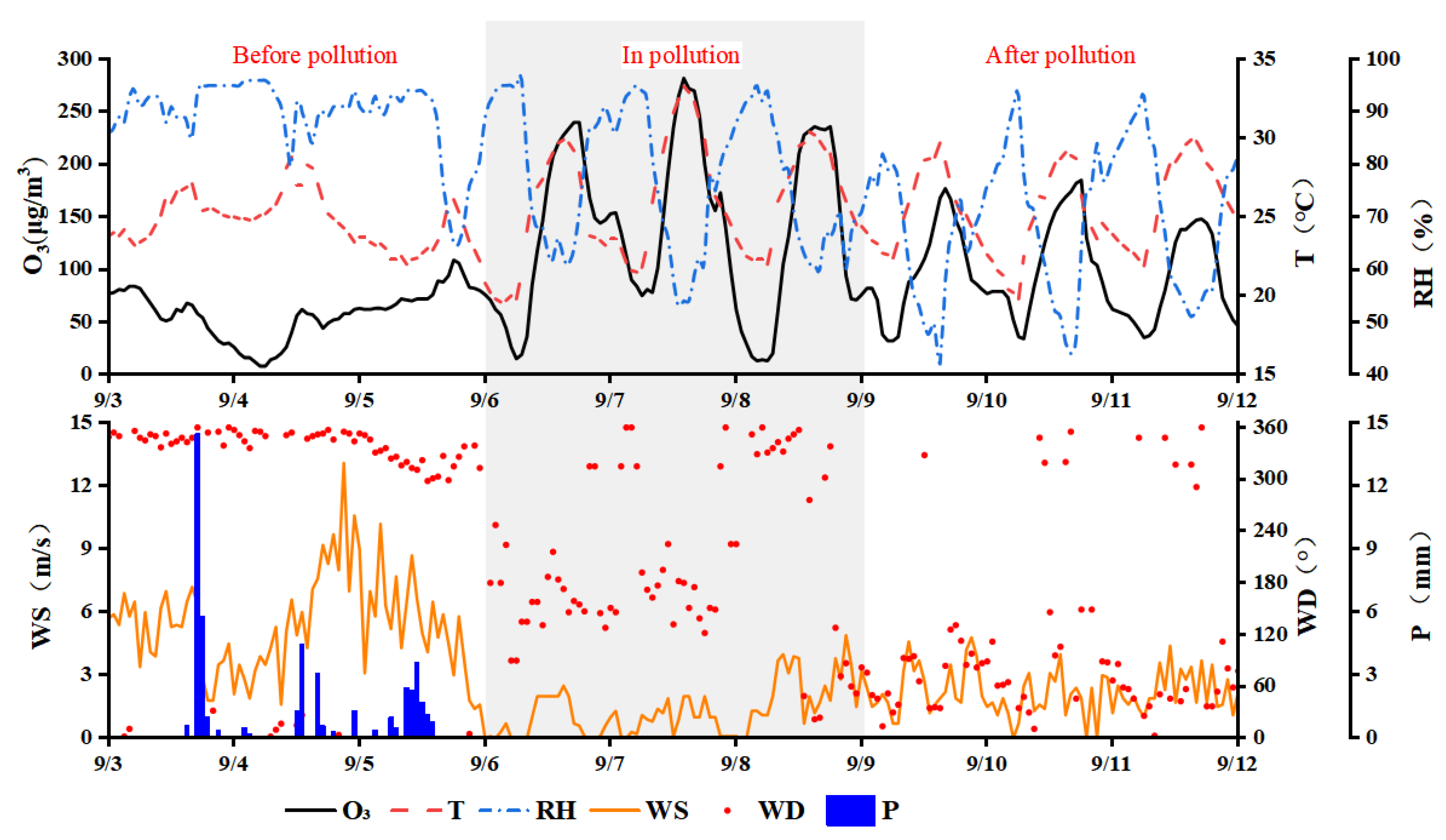
3.1. Pollution Profile and Meteorological Characteristics

From 3–11 September 2022, Jiaxing City experienced an O₃ pollution event coinciding with Typhoon Xuanlannuo (see Figure 2). During the periods of 6– September and 10 September, the maximum 8 h average O₃ concentration exceeded standards for a total of 4 days. This pollution episode was prolonged and moderate, with the maximum 8 h sliding average O₃ concentration exceeding 200 μg/m³ from 6–9 September , indicating a moderate pollution level (level 4). The average concentration range was between 220 μg/m³ and 246 μg/m³. Notably, on 7 September, the maximum hourly O₃ concentration reached 282 μg/m³, which surpasses the 1 h concentration limit of 200 μg/m³ specified in China’s ambient air quality standards (GB3095-2012) by 41%. The O₃ concentration exhibited a distinct “low-high-low” pattern, allowing the pollution process to be categorized into three phases: before pollution (3–5 September), during pollution (6–8 September), and after pollution (9–11 September).

Before the onset of pollution, Jiaxing City exhibited excellent air quality. The city was located on the western periphery of Typhoon Xuanlannuo (Figure S1) and was surrounded by the typhoon’s peripheral cloud system (see Figure S2). As a result, the shortwave radiation incident to the Earth’s surface was significantly reduced (see Figure S3). The maximum temperature remained below 28.8 °C (Figure S4), while the average relative humidity reached an exceptionally high 89.4% (

Table 1. Meteorological elements of Jiaxing City, 3–11 September.

Stage	Temperature (°C)			Wind Speed (m/s)			Relative Humidity (%)			Precipitation (mm)
	Max	Min	Average	Max	Min	Average	Max	Min	Average	Cumulative
Before pollution	28.8	22.0	24.7	13.1	1.4	5.4	96.5	65.2	89.4	48.0
Polluted	33.3	19.6	25.9	4.9	0.0	1.3	96.4	53.1	77.0	0.0
After pollution	29.9	19.8	25.4	4.8	0.0	2.2	96.3	43.1	69.0	0.0

). These conditions diminished the intensity of photochemical reactions, making ozone generation less favorable. Robust convective activity promoted low atmospheric stability within the typhoon’s circulation, facilitating vertical pollutant dispersion. Surface winds primarily blew from the north, with average wind speeds between levels 3 and 4 (Table 1). This wind pattern aided in the horizontal dilution and dispersion of pollutants. The typhoon’s cloud system also produced precipitation (see Figure S5), leading to rainfall over three to five days. On 3 September, cumulative rainfall reached 22.6 mm, a moderate amount effective in removing pollutants.

In terms of pollution, the air quality in Jiaxing City is moderately polluted, and the primary pollutant is ozone. From the perspective of meteorological conditions, the typhoon circulation moves northeast, Jiaxing City gradually becomes controlled by high pressure from the rear of the typhoon (see Figure S1), and the cloud system above becomes thinner (see Figure S2). The intensity of incident shortwave radiation on the ground increases significantly (see Figure S3), and the temperature near the ground increases significantly, with the daily maximum temperature reaching over 32 °C (see Figure S4). The relative humidity dropped considerably during the day, and the relative humidity was less than 60% in the afternoon, which is very conducive to photochemical reactions. At the same time, dynamically, high pressure prevails at the rear of the typhoon, and downdrafts prevail. Convection activities weaken, atmospheric stability increases, southerly winds near the surface occur, and wind power decreases significantly. The hourly average wind speed is only 1.28 m/s (Table 1). The vertical and horizontal directions are not conducive to pollutant dispersion and dilution. In addition, high-temperature, sunny, and hot weather occurs under high-pressure downdrafts without precipitation (see Figure S5), which is not conducive to the wet deposition of pollutants.

After the pollution (9–11 September), Jiaxing City’s air quality was slightly polluted for 1 day and suitable for 2 days. From the perspective of meteorological conditions, as Typhoon “Xuanlannuo” gradually moves northward, the high-pressure belt follows suit and further moves northward. Simultaneously, a new tropical cyclone forms on the south side of the high-pressure belt. This development further weakens the high-pressure belt’s control over the Jiaxing area (see Figure S1, bottom). Consequently, the cloud system over Jiaxing increases (see Figure S2), the incident short-wave radiation on the surface weakens (see Figure S3), and the daily temperature near the surface drops as well, with the maximum temperature falling to around 30 °C. As a result, the photochemical reaction becomes weaker compared to the polluted situation, and the ozone generation rate decreases. Dynamically, the northward-lifting downdraft of the high-pressure belt weakened, the atmospheric stability decreased, and the near-surface winds also strengthened. The average wind speed increased to 2.20 m/s. Pollutant dispersion conditions in vertical and horizontal directions have improved, and ozone concentration has declined. The pollution level is reduced, and the air quality turns good or is lightly polluted.

Comparing the meteorological conditions in the three periods, it was found that the ozone pollution period mainly had the following four characteristics: (1) controlled by high pressure at the rear of the typhoon, downdrafts prevailed, and the vertical pollutant dispersion was unfavorable; (2) the temperature rose significantly, the daily relative humidity was significantly reduced, and the local photochemical reaction intensity was high; (3) the surface wind speed was obviously low, there was no rainfall process, the weather was stable, and the pollutant dispersion in the horizontal direction was unfavorable; (4) it was in the wind field convergence zone for a long time, local ozone precursors and pollutants such as O₃ accumulated rapidly and locally remained at high values for a long time.

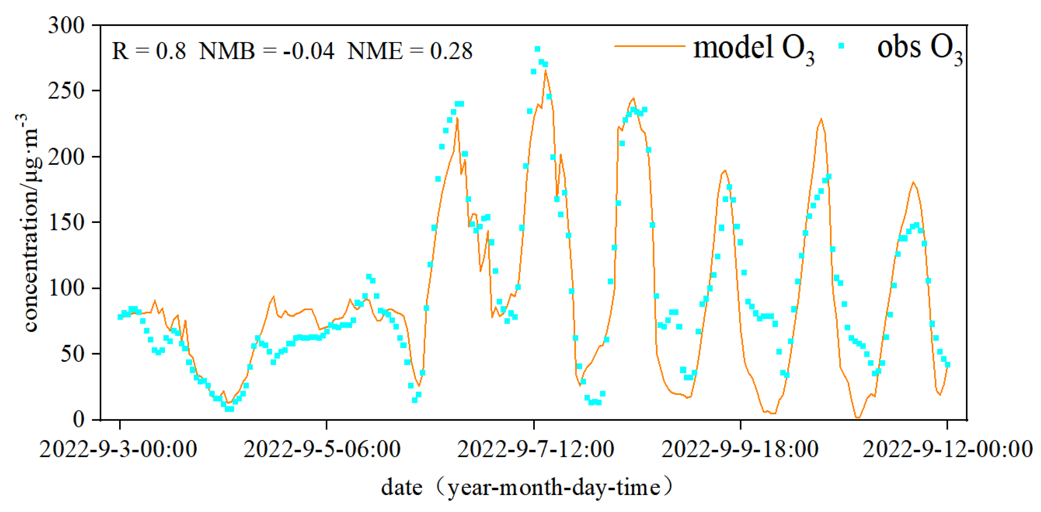
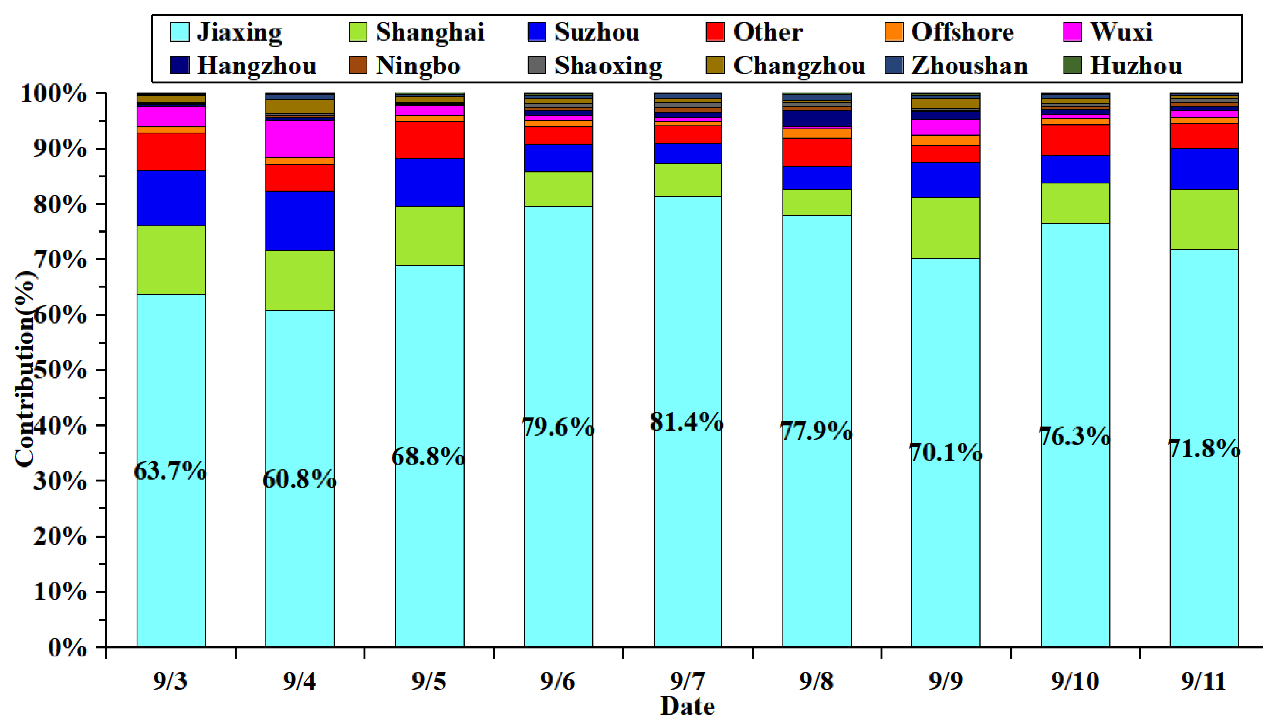
3.2. Model Simulation Verification and Regional Contribution of Ozone During Typhoon

In this study, the Weather Research and Forecasting (WRF) model, specifically version v3.9.1, was employed. The simulation utilized the Lambert conformal conic projection. To mitigate grid distortion associated with the projection method and ensure that the entirety of the Chinese region was centered within the simulation domain, two standard parallels were selected at 25° N and 40° N, with the domain’s central coordinates set at (30.79° N, 120.80° E). The grid configuration consists of 245 grid points in the west-to-east direction and 195 grid points in the south-to-north direction, with a uniform grid resolution of 27 km × 27 km. In the vertical dimension, the meteorological simulation extends to a top-level pressure of 100 mb. The atmosphere from the surface to the top of the model layer is discretized into 24 sigma (σ) levels, namely, 1.000, 0.995, 0.988, 0.980, 0.970, 0.956, 0.938, 0.916, 0.893, 0.868, 0.839, 0.808, 0.777, 0.744, 0.702, 0.648, 0.582, 0.500, 0.400, 0.300, 0.200, 0.120, 0.052, and 0.000. For the simulation, terrain and land-surface type data were sourced from the Moderate Resolution Imaging Spectroradiometer (MODIS) satellite dataset provided by the National Aeronautics and Space Administration (NASA). The first-guess field was derived from the ds083.2 global reanalysis dataset provided by the National Centers for Environmental Prediction (NCEP). This dataset features a horizontal resolution of 1 × 1 and a temporal resolution of 6 h. To enhance the accuracy of the simulated meteorological outcomes, a four-dimensional data assimilation (FDDA) approach was applied to the WRF model. The assimilation incorporated observational data from two datasets: the ds461.0 dataset of global surface-based meteorological observations from international exchange stations and the ds351.0 global radiosonde observational dataset. To assess the model’s performance, various statistical indices were used, including the simulated mean (MeanSim), observed mean (MeanObs), mean bias (MB), gross error (GE), root mean square error (RMSE), and index of agreement (IOA). These metrics comprehensively evaluate the model’s accuracy in simulating meteorological conditions.

Table 2. Calibration results of Jiaxing Meteorological Field from 2–11 September 2022.

	T (°C)	Wdir (deg)	Wspd (m/s)	RH (%)
Mean Obs	25.34	201.76	2.96	78.61
Mean Sim	25.54	134.32	3.51	77.15
MBs	−0.20	67.45	−0.55	1.46
Gross Error	3.25	108.62	1.47	6.23
RMSE	4.17	/	1.83	8.33
IOA	0.78	/	0.78	0.92

presents the calibration results of the meteorological simulations compared to observed values. Based on the recommended calibration standards, the simulated wind speed (within ±0.5 m/s), wind direction (within ±10°), and humidity (within ±1 g/kg) all fall within acceptable error margins. Overall, the WRF model’s meteorological simulations align well with near-surface observations and effectively reproduce the meteorological conditions. For air quality calibration, hourly O₃ observations from national monitoring stations published by the China National Environmental Monitoring Center (CNEMC) were compared with the WRF-CMAQ simulation results. The statistical parameters used to evaluate the performance of the WRF-CMAQ system include the Normalized Mean Bias (NMB), Normalized Mean Error (NME), and Correlation Coefficient (R). The spatial distribution characteristics of the simulated and observed O3 concentrations (marked by dots in the Figure 3) are shown. Overall, the WRF-CMAQ simulation system can reproduce the air pollution process well and capture the spatial distribution characteristics of air pollutant concentrations in the simulation domain.

The quantitative outcomes derived from the CMAQ-ISAM model indicate that from September 3 to 11, the local concentration contribution in Jiaxing ranged from 60.8% to 81.4% (see Figure 4). The average contribution was substantial at 72.3%, establishing it as the primary source of ozone. Notably, this contribution displayed a commendable level of stability. In contrast, external sources contributed between 18.6% and 39.2% to Jiaxing’s ozone levels. Minor contributors among these external sources included the cities of Hangzhou, Zhoushan, Shaoxing, and Ningbo within Zhejiang Province. Additionally, cities beyond the provincial borders, such as Shanghai, Suzhou, and Wuxi, played a considerable role. Specifically, Shanghai contributed between 4.8% and 12.3%, while Suzhou’s contribution ranged from 3.7% to 10.6%. Analyzing distinct pollution periods (see Figure 5), it is evident that the local contribution in Jiaxing peaked at 79.6%. This figure exceeded both pre-pollution and post-pollution levels, underscoring the contribution of local pollution source emissions to the formation of O₃ pollution.

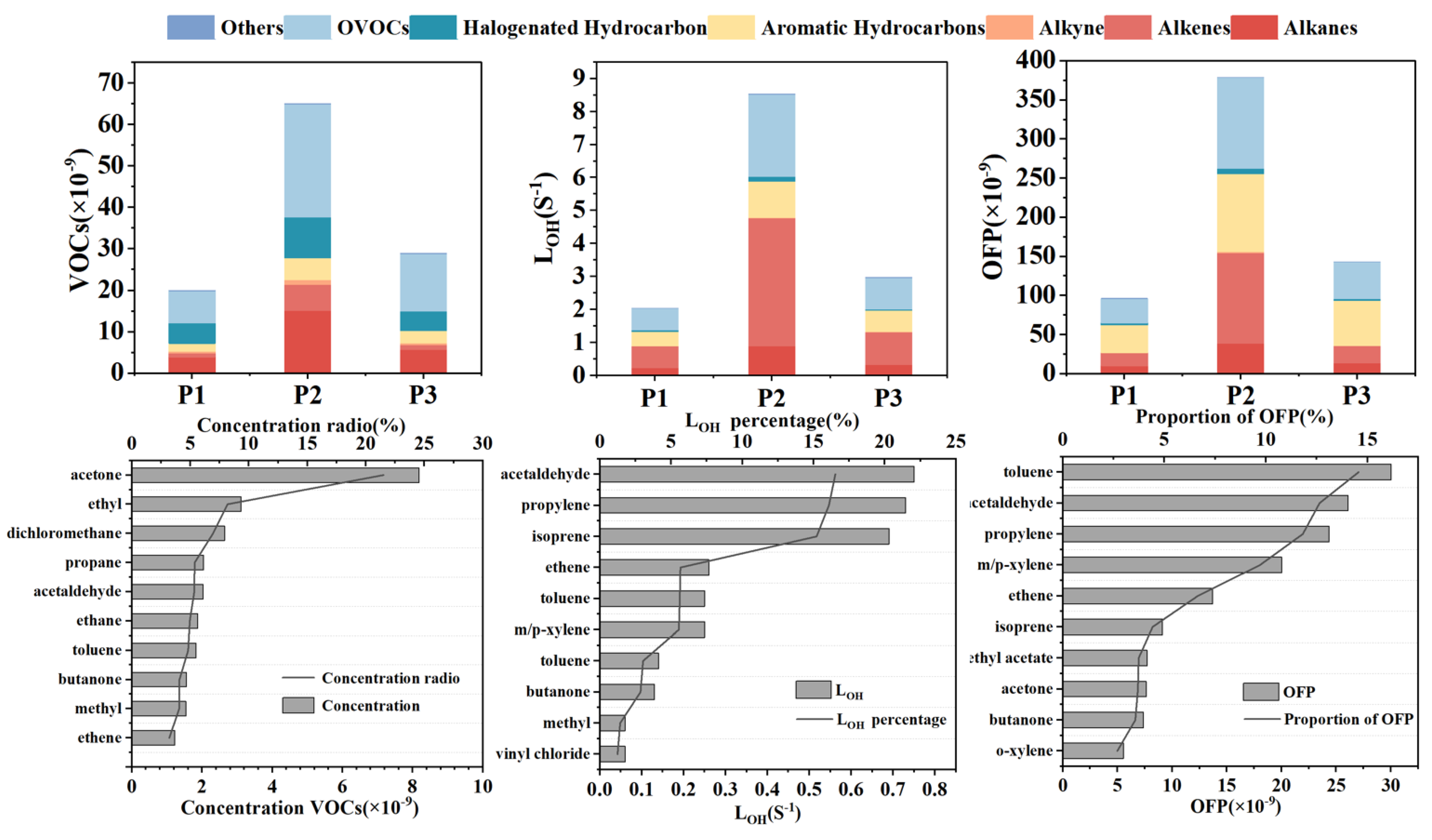
3.3. Identification of Key VOCs in Ozone Formation

VOCs are vital contributors to ozone formation in the atmosphere through complex photochemical reactions [34]. In this study, we utilized the consumption rate of OH in the atmosphere to estimate the chemical reactivity of VOC substances, providing a simple indicator for investigating the relative contribution of VOCs to the daytime photochemical reactions. Meanwhile, the OFP was employed to quantify the contribution of VOCs to ozone formation, reflecting the maximum capacity of ozone generation possessed by VOCs in the atmosphere. Figure 6 presents the chemical composition of VOCs, the reactive composition of OH, and the ozone generation potential composition in Jiaxing City during the observation period. The average volume fraction of VOCs in Jiaxing City was 38.0 × 10⁻⁹. Among these, the distribution included alkanes at 8.2 × 10⁻⁹, olefins at 2.8 × 10⁻⁹, acetylene at 0.7 × 10⁻⁹, and aromatic hydrocarbons at 3.4 × 10⁻⁹. Additionally, halogenated hydrocarbons accounted for 6.5 × 10⁻⁹, OVOCs comprised 16.3 × 10⁻⁹, and carbon disulfide contributed 0.14 × 10⁻⁹. Notably, OVOCs emerged as the primary components, constituting 43.0% of the total VOCs, followed by alkanes at 21.6% and halogenated hydrocarbons at 17.0%. Although olefins and aromatic hydrocarbons were in lower concentrations, they exhibited heightened chemical reactivity, significantly impacting their ozone formation potential. Specifically, olefins contributed 40.9% to the L_OH and 25.0% to the OFP, establishing them as the primary contributors to LOH. Meanwhile, aromatic hydrocarbons accounted for 16.0% of L_OH and 31.2% of OFP, making them the second-highest contributor to ozone generation. In conclusion, olefins and aromatic hydrocarbons were crucial in ozone generation in Jiaxing City.

When assessing changes in chemical composition during each pollution period (see Figure 6), it becomes evident that the concentrations of VOCs, OH reactivity, and ozone formation potential were significantly higher during pollution than before and after. Among these, OVOCs and alkanes exhibited the most substantial increases. Regarding OH reactivity, olefins and OVOCs experienced the most significant surge in LOH. As for ozone generation potential, olefins, aromatic hydrocarbons, and OVOCs displayed the most noticeable changes (see Figure 6). In terms of concentration control, acetone, ethyl acetate, dichloromethane, propane, acetaldehyde, ethane, toluene, butanone, methyl chloride, and ethylene have accounted for the highest concentration contributions, totaling 68.4% of the overall composition.

Regarding ozone prevention and control, key VOCs responsible for ozone issues primarily comprised olefins and aromatic hydrocarbons. Toluene, acetaldehyde, propylene, m-p-xylene, ethylene, isoprene, and ethyl acetate were the species with substantial contributions to L_OH and OFP. Notably, ethylene, propylene, and isoprene significantly surpassed other species in LOH contributions. In contrast, toluene, ethylene, propylene, and m-p-xylene contributed substantially to OFP, marking them as pivotal species in ozone pollution control within Jiaxing.

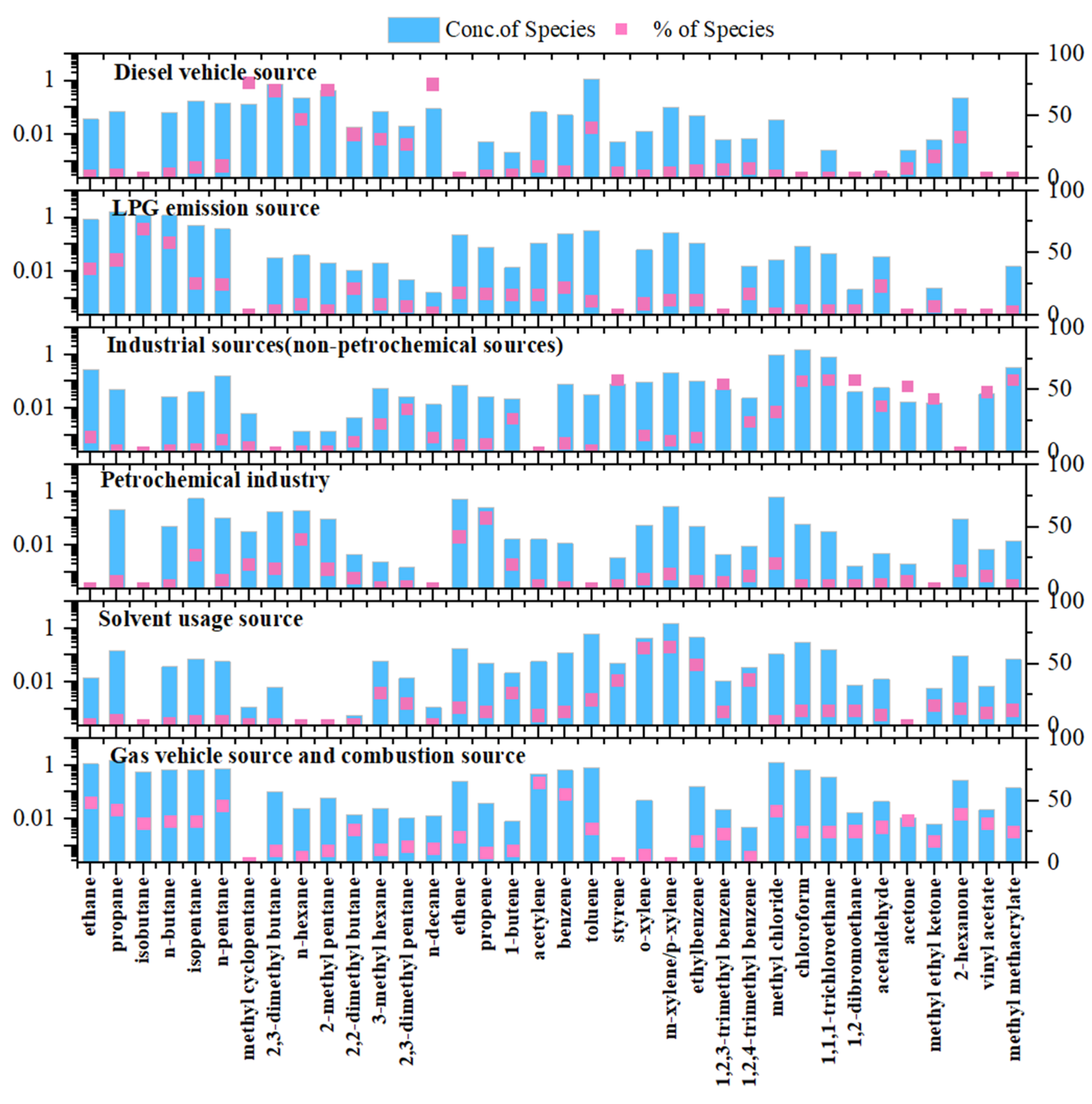
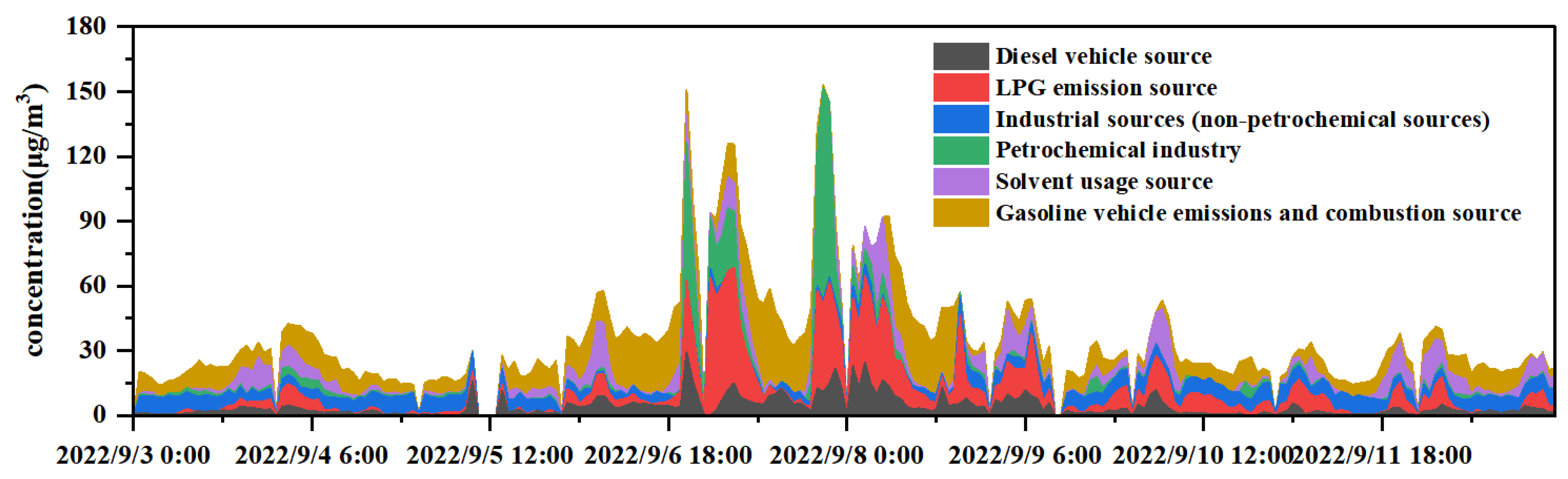
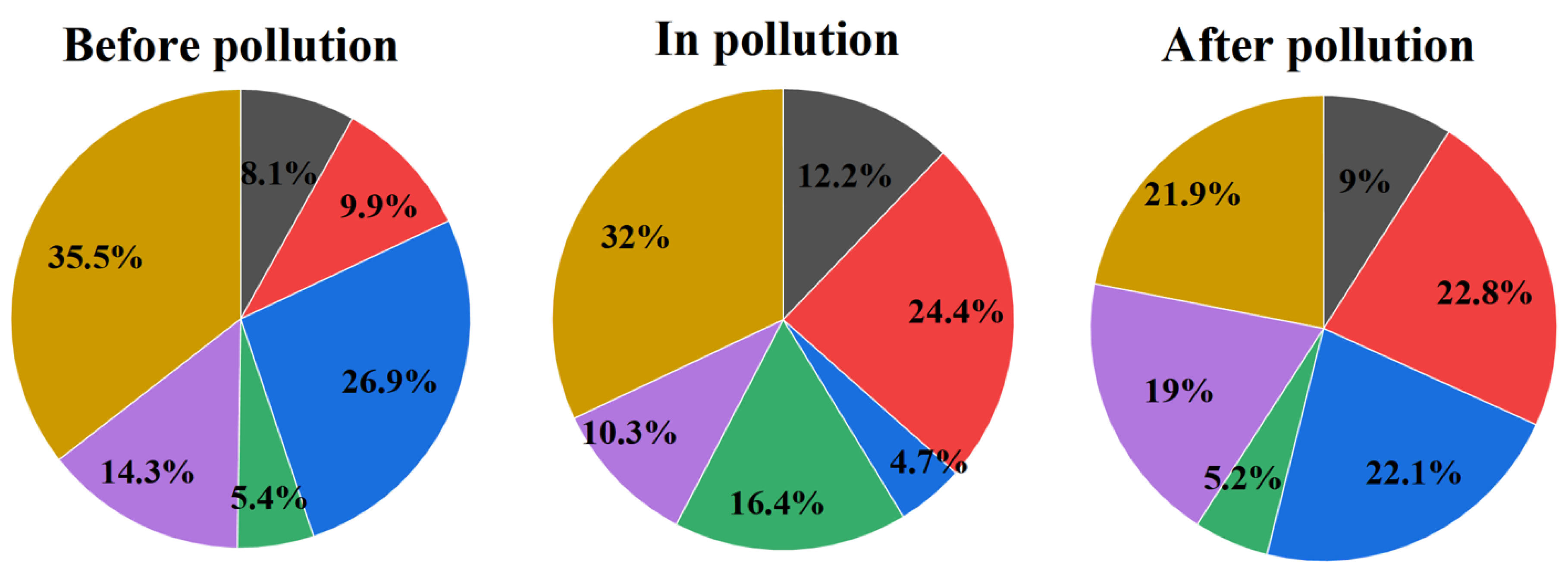
3.4. Analysis of the Source of Ozone Precursor (VOCs) During Typhoon

For the analysis of the sources of VOCs monitored at the photochemical component site during the pollution period, we employed the positive matrix factorization (PMF) receptor model. To ensure the model’s reliability, we observed the change trend from 3 factors to 11 factors (Qtue/Qexp) and found that the rate of change (Qtrue/Qexp) remained below 10% for 6 factors. Additionally, the majority of residual values for each species fell within the range of ±3, indicating scattered sources and enhanced model stability. Consequently, determining six factors was deemed the optimal operational choice for PMF. The profiles of the factors derived from the six-factor solution are presented in Figure 7. The concentration of each species is apportioned to each factor and indicated in blue, and the percentage accounted for by each species in the factor is indicated by a red square. The concentrations corresponding to the y-axis on the left are expressed in the logarithmic scale, and the percentage explained by the factor for each species must be found in the y-axis on the right. The six factors have been identified as sources of VOCs based on the resulting emission profile markers as explained below.

The main characteristic VOC species of factor 1 are high-carbon alkanes such as methylcyclopentane, 2,3-dimethylbutane, n-hexane, and n-decane, which contain a relatively high concentration of toluene. In the study of the VOC emission spectra of diesel vehicles in China, toluene and long-chain alkanes such as n-decane, undecane, and dodecane can be used as tracers for diesel vehicle emissions [35]. So, factor 1 is identified as the diesel vehicle emission source. Factor 2 was identified as liquefied petroleum gas (LPG) emission source, and the main species are propane, isobutane, and n-butane. LPG is a mixture of propane and butane. Ahmed found that propane is the main tracer of LPG emissions in Houston [36]. Meanwhile, this factor does not contain combustion species such as low-carbon olefins, alkynes, and toluene, and the source is not the combustion process. So, factor 2 is recognized as the LPG emission source. Factor 3 is attributed to industrial emission sources (non-petrochemical sources). Its characteristic lies in the fact that the main species include chloromethane, trichloromethane, trichloroethane, styrene, and trimethylbenzene. According to the monitoring results of industrial parks in the Yangtze River Delta [37], aromatic hydrocarbons, halogenated hydrocarbons, and OVOCs are the main components. Among them, halogenated hydrocarbons make a considerable contribution in industries such as rubber manufacturing and the electronic industry, and aromatic hydrocarbons and OVOCs contribute significantly in the surface coating industry [38]. There are numerous industrial enterprises around the observation site, involving industries including rubber manufacturing, the textile industry, the metal processing industry, etc. So, factor 3 is identified as industrial emission sources (non-petrochemical sources). The major VOC species of factor 4 were ethene and propene. The relative contributions of this factor to ethene and propene were 41.6% and 56.8%, respectively. Alkenes are the key raw materials and products of the petrochemical industry [39]. Meanwhile, to the south and upwind of the observation site, there is a petrochemical production base. So, factor 4 is identified as petrochemical industry. Factor 5 has characteristic species of C7–C9 aromatic hydrocarbons: toluene, ethylbenzene, m/p-xylene, o-xylene, and 1,2,4-trimethylbenzene. Existing studies have shown that a large number of aromatic hydrocarbons are emitted during the processes of coating and solvent usage [37,40]. So, factor 5 is identified as a solvent usage source. The main characteristics of factor 6 are low-carbon alkanes, olefins, and alkynes such as ethane, propane, butane, pentane, and ethylene, as well as aromatic hydrocarbons such as benzene and toluene. In most studies, ethane, ethylene, isopentane, 2-methyl ethane, toluene, and benzene are the main components of gasoline vehicle emissions in China. Moreover, acetylene, benzene, and toluene are also the products of combustion emissions. Therefore, factor 6 also has some characteristics of the combustion source. So, factor 6 is identified as a mixed source of gasoline vehicle emissions and combustion.

Throughout the pollution period, emissions from sources, excluding industrial sources (non-petrochemical), exhibited a significant increase, ranging from 0.98 to 7.36 times higher. Both the emissions and contributions of industrial sources (petrochemical) and liquefied petroleum gas (LPG) witnessed a notable surge compared to the pre-pollution levels. Examining the daily variation in the contribution rates of various VOC sources during the observation period (see Figure 8), it is noteworthy that industrial sources (petrochemical chemicals) and LPG sources experienced a substantial increase in their combined contribution, reaching a remarkable 54.3% on the 7th day. Consequently, industrial sources (petrochemical chemicals) and LPG sources emerge as pivotal sources for VOC control during O₃ pollution episodes in Jiaxing.

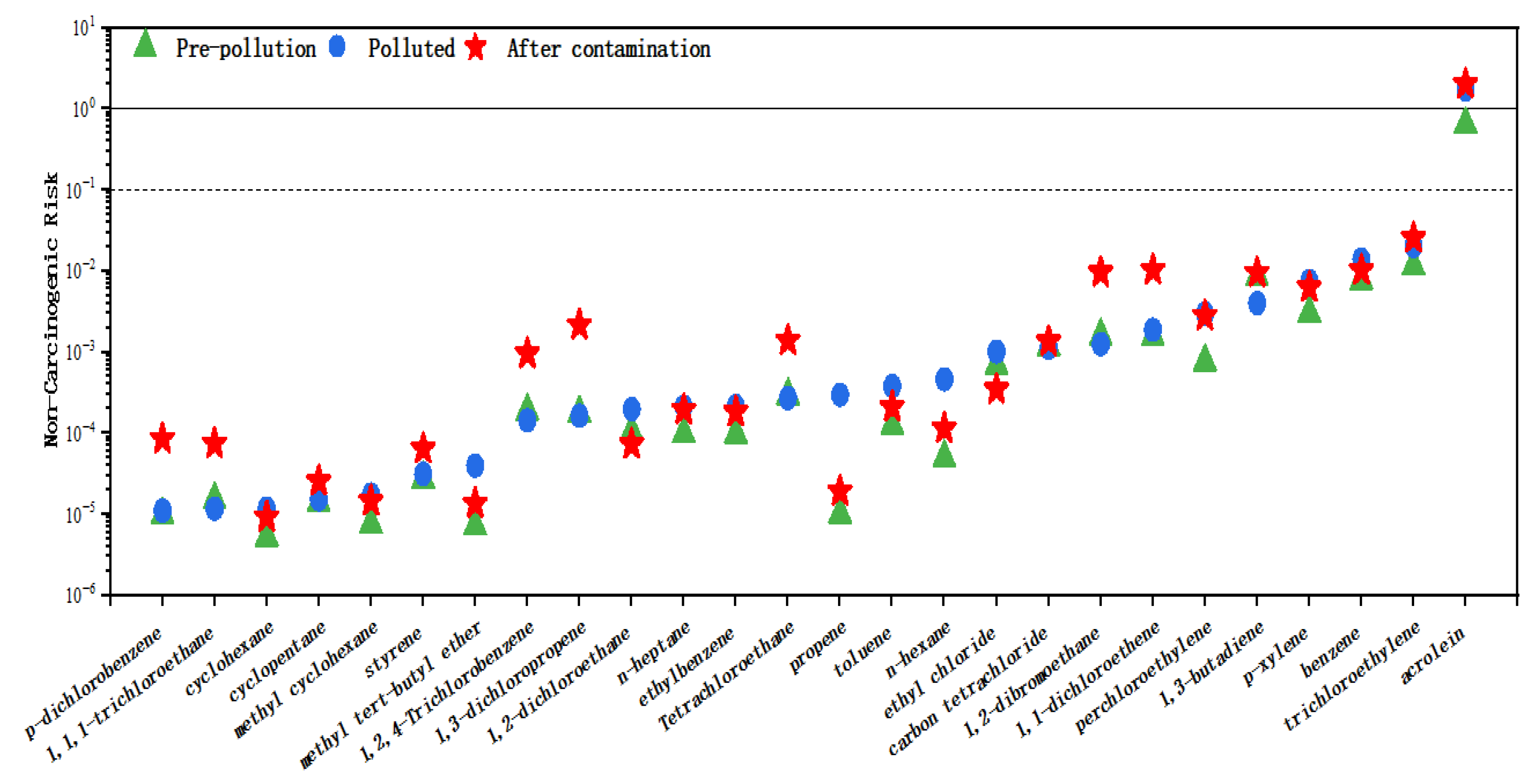
3.5. Ozone Precursor (VOCs) NCR Health Risk Assessment and LCR Health Risk Assessment During Typhoon

According to the average mass concentration of toxic VOCs during different ozone pollution periods in Jiaxing City under the influence of the typhoon weather system, combined with the respiratory exposure habits of Chinese people, an NCR health risk assessment was carried out (see Figure 9). The results showed that the total HI values during the monitoring period were 0.685, 1.80, and 2.10 during the pre-pollution period, during the pollution period, and after the pollution period, respectively, indicating that the total HI values during the middle and late stages of pollution were more significant than the safety threshold recommended by the US EPA (NCR = 1) [15]. The risk of non-carcinogenicity in the late stage of pollution was higher than in the period before and after. Further analysis showed that the NCR values of acrolein during and after pollution exceeded the safety thresholds recommended by the US EPA, reaching 1.74 and 2.02, respectively. In contrast, the remaining 25 substances did not exceed the US EPA’s recommended values, indicating a non-carcinogenic risk in Jiaxing during and after pollution, and acrolein in the regional environment was the culprit of chronic non-carcinogenic risk.

The LCR health assessment was performed based on the average mass concentrations of toxic VOCs during different ozone pollution periods in Jiaxing City under the influence of a typhoon weather system, combined with the respiratory exposure habits of the Chinese population. The data showed (see Figure 10) that the total HI values during the monitoring period were 1.03 × 10⁻⁵, 1.78 × 10⁻⁵, and 1.03 × 10⁻⁵ in the pre-pollution, mid-pollution, and post-pollution periods, respectively, suggesting that the total HI values in the pre-pollution, mid-pollution, and post-pollution periods were all greater than the safety threshold indicated by the US EPA (LCR = 10⁻⁶), and the cancer risk in the mid-pollution period was higher than the pre- and post-pollution periods risk by a factor of 1.73. Further analysis revealed that 1,2-dichloroethane and benzene had LCR values ranging from 1.8 × 10⁻⁶ to 1.24 × 10⁻⁵, which were more significant than the safety thresholds suggested by the US EPA before, during, and after the contamination. The highest concentrations were found in the mid-time contamination period, the primary substance causing the carcinogenicity risk. In contrast, the rest of the substances did not exceed the safety thresholds suggested by the US EPA.

3.6. Control Strategies for Ozone Pollution Episodes During Typhoon

During the pollution period in Jiaxing City, there was a significant elevation in ozone concentration, posing a grave threat to air quality and public health. This issue has garnered theoretical attention and yielded tangible consequences in practice. Consequently, there is an urgent need for a comprehensive understanding of the sources and characteristics of volatile organic compounds (VOCs). Employing a receptor model with positive feedback methodology, we have effectively analyzed the origins of VOCs during the pollution period in Jiaxing City.

VOCs are vital contributors to ozone formation in the atmosphere through complex photochemical reactions. These compounds react with nitrogen oxides (NOx) in the presence of sunlight to produce ozone, a process known as photochemical smog formation. Therefore, elucidating the sources of VOCs is crucial for mitigating ozone pollution and improving air quality. Our analysis during the pollution period identified six major source factors contributing to VOC emissions in Jiaxing City. These sources encompassed a range of industrial, vehicular, and residential activities known to emit VOCs into the atmosphere.

Primarily, we underscore the dominant influence of VOCs on ozone generation. A thorough elucidation of VOC sources is of paramount importance for the effective control of ozone pollution. This perspective finds extensive international affirmation as numerous cities and regions have successfully implemented VOC control strategies, significantly enhancing air quality and reducing ozone-related health risks [41,42,43,44]. For instance, a 40% reduction in emissions from the dominant VOC source (i.e., paint and sealant solvents) was demonstrated to yield the highest ozone (O₃) abatement efficiency for this source in Hong Kong [42]. This conclusion aligned with findings from Heather Simon, who demonstrated that the highest U.S. ozone concentrations have been reduced over the past 15 years in response to a substantial decrease in ozone precursor emissions [41]. We have unambiguously identified six major VOC source factors throughout the pollution period. This analysis dramatically aids in pinpointing the contributions of individual pollution sources, thereby providing vital clues for the formulation of targeted control strategies. Notably, it is imperative to recognize that certain negative instances underscore the indispensability of comprehensive VOC source analysis in addressing seemingly insurmountable ozone pollution challenges.

Industrial activities, particularly petrochemicals, emerged as significant contributors to VOC emissions during the pollution episode. Petrochemical plants release a variety of VOCs during their manufacturing processes, including benzene, toluene, ethylbenzene, and xylene (BTEX compounds), which are potent precursors to ozone formation. The production, processing, and storage of petrochemicals entail various VOC-emitting activities, such as storage tank emissions, fugitive emissions from equipment leaks, and chemical processes. Industrial combustion processes, such as boilers and furnaces, also release VOCs into the atmosphere. These industrial emissions constitute a substantial portion of total VOC emissions and require targeted control measures for effective pollution reduction.

Diesel vehicle emissions predominantly consist of high-carbon alkanes and toluene, aligning conspicuously with the characteristics of diesel exhaust emissions. Consequently, diesel vehicles have been unequivocally designated as a critical source of VOC pollution in Jiaxing City. This conclusion finds robust support from a series of affirmative cases where cities have effectively implemented measures to control diesel vehicle emissions, resulting in a substantial reduction in VOC emissions and corresponding improvements in air quality. However, liquefied petroleum gas (LPG) emissions primarily encompass propane, isobutane, and butane, aligning closely with LPG composition. This indicates the significant role played by LPG use in VOC emissions. Affirmative cases indicate that effective LPG usage management measures have reduced VOC emissions and improved air quality in certain regions.

In summary, industrial sources (petrochemical industry) and LPG sources experienced the most substantial increase in VOC emissions during the ozone pollution period. Consequently, these two sources warrant heightened attention. Successful cases demonstrate that measures to reduce VOC emissions from these sources hold the potential to lower ozone pollution levels effectively, enhance air quality, and thereby better safeguard public health. Furthermore, we refined the calculations of carcinogenic and non-carcinogenic risks by incorporating the unique respiratory exposure habits of the Chinese population. Health risk assessments have unveiled that acrolein plays a predominant role in chronic non-carcinogenic risks within regional environments. Notably, during and subsequent to ozone pollution episodes, the non-carcinogenic risk (NCR) values for acrolein soar to 1.74 and 2.02, respectively. However, in the context of carcinogenic risk assessment, the cancer risk during the mid-point of pollution events is 1.73 times higher than the risks associated with pre- and post-pollution periods, with this escalation primarily attributed to the pollutants 1,2-dichloroethane and benzene.

4. Conclusions

The O₃ pollution process in Jiaxing City is closely related to meteorological conditions. During the pollution period, it is controlled by the high-pressure sinking air flow after the typhoon is far away, and the weather of sunny heat, high temperature, low humidity, and light wind occurs, which is very conducive to the generation and accumulation of local O₃. In addition, there is no continuous wind direction during the pollution period, and the frequency of southerly wind is high, which is conducive to the transport of ozone and its precursors, aggravating pollution. Local generation is the most crucial source of Jiaxing O₃. During the observation period, Jiaxing’s local source contribution was about 72.3%. During the O₃ pollution period, the contribution of local sources accounted for about 79.6%, an increase of 15.2% and 6.8%, respectively, compared with the two periods before and after pollution, so Jiaxing should further strengthen the control of local sources. Among VOCs, olefins and aromatic hydrocarbons contribute significantly to ozone formation in Jiaxing. During the pollution period, VOCs and NOX increased significantly, and the concentration of O₃ increased. Among VOCs, olefins and aromatic hydrocarbons had a more significant impact on ozone formation in Jiaxing, olefins and aromatic hydrocarbons contributed relatively well to LOH and OFP, olefins contributed 40.9% and 25.0% to LOH and OFP, and aromatic hydrocarbons accounted for 16.0% and 31.2%, respectively. For the ozone precursor VOCs in the entire pollution process, a total of six significant sources were analyzed, namely, diesel vehicle emission sources, LPG emission sources, industrial sources (non-petrochemical chemicals), industrial sources (petrochemical chemicals), solvent-use sources, and gasoline vehicle emission sources. Among them, industrial sources (petrochemical chemicals) and LPG sources increased significantly during the pollution period, which was the primary source of VOC control during O₃ pollution in Jiaxing. The health risk evaluations have demonstrated that acrolein is a significant contributor to chronic non-carcinogenic risks in regional settings. Strikingly, both during and following the ozone pollution incidents, the non-carcinogenic risk (NCR) values for acrolein escalate significantly to 1.74 and 2.02, respectively. Conversely, within the framework of carcinogenic risk assessment, the midpoint of pollution events exhibits a cancer risk that is 1.73 times greater than those during the periods preceding and succeeding the pollution, with this increase predominantly linked to the pollutants 1,2-dichloroethane and benzene. Thus, this study furnishes a robust scientific foundation for air quality management in Jiaxing City, underscoring the imperative need for requisite policies and actions.

References

1. Staehelin, J.; Harris, N.R.P.; Appenzeller, C.; Eberhard, J. Ozone trends: A review. Rev. Geophys. 2001, 39, 231–290. [Google Scholar] [CrossRef]
2. Bernhard, G.H.; Bais, A.F.; Aucamp, P.J.; Klekociuk, A.R.; Liley, J.B.; McKenzie, R.L. Stratospheric ozone, UV radiation, and climate interactions. Photochem. Photobiol. Sci. 2023, 22, 937–989. [Google Scholar] [CrossRef]
3. Wilson, S.R.; Madronich, S.; Longstreth, J.D.; Solomon, K.R. Interactive effects of changing stratospheric ozone and climate on tropospheric composition and air quality, and the consequences for human and ecosystem health. Photochem. Photobiol. Sci. 2019, 18, 775–803. [Google Scholar] [CrossRef]
4. Seinfeld, J.H.; Pandis, S.N. Atmospheric Chemistry and Physics: From Air Pollution to Climate Change; John Wiley & Sons: Hoboken, NJ, USA, 2016. [Google Scholar]
5. Fowler, D.; Amann, M.; Anderson, R.; Ashmore, M.; Cox, P.; Depledge, M.; Derwent, D.; Grennfelt, P.; Hewitt, N.; Hov, O. Ground-Level Ozone in the 21st Century: Future Trends, Impacts and Policy Implications; The Royal Society: London, UK, 2008. [Google Scholar]
6. Monks, P.S.; Archibald, A.T.; Colette, A.; Cooper, O.; Coyle, M.; Derwent, R.; Fowler, D.; Granier, C.; Law, K.S.; Mills, G.E.; et al. Tropospheric ozone and its precursors from the urban to the global scale from air quality to short-lived climate forcer. Atmos. Chem. Phys. 2015, 15, 8889–8973. [Google Scholar] [CrossRef]
7. Ma, T.; Duan, F.K.; He, K.B.; Qin, Y.; Tong, D.; Geng, G.N.; Liu, X.Y.; Li, H.; Yang, S.; Ye, S.Q.; et al. Air pollution characteristics and their relationship with emissions and meteorology in the Yangtze River Delta region during 2014-2016. J. Environ. Sci. 2019, 83, 8–20. [Google Scholar] [CrossRef] [PubMed]
8. Zhang, X.; Ma, Q.; Chu, W.; Ning, M.; Liu, X.; Xiao, F.; Cai, N.; Wu, Z.; Yan, G. Identify the key emission sources for mitigating ozone pollution: A case study of urban area in the Yangtze River Delta region, China. Sci. Total Environ. 2023, 892, 164703. [Google Scholar] [CrossRef]
9. Hu, F.; Xie, P.; Zhu, Y.; Zhang, F.; Xu, J.; Lv, Y.; Zhang, Z.; Zheng, J.; Zhang, Q.; Li, Y. The impact of evolving synoptic weather patterns on multi-scale transport and sources of persistent high-concentration ozone pollution event in the Yangtze River Delta, China. Sci. Total Environ. 2024, 949, 175048. [Google Scholar] [CrossRef]
10. Xie, M.; Liao, J.B.; Wang, T.J.; Zhu, K.G.; Zhuang, B.L.; Han, Y.; Li, M.M.; Li, S. Modeling of the anthropogenic heat flux and its effect on regional meteorology and air quality over the Yangtze River Delta region, China. Atmos. Chem. Phys. 2016, 16, 6071–6089. [Google Scholar] [CrossRef]
11. Qi, C.; Wang, P.; Yang, Y.; Li, H.; Zhang, H.; Ren, L.; Jin, X.; Zhan, C.; Tang, J.; Liao, H. Impacts of tropical cyclone–heat wave compound events on surface ozone in eastern China: Comparison between the Yangtze River and Pearl River deltas. Atmos. Chem. Phys. 2024, 24, 11775–11789. [Google Scholar] [CrossRef]
12. Zhan, C.; Xie, M.; Huang, C.; Liu, J.; Wang, T.; Xu, M.; Ma, C.; Yu, J.; Jiao, Y.; Li, M.; et al. Ozone affected by a succession of four landfall typhoons in the Yangtze River Delta, China: Major processes and health impacts. Atmos. Chem. Phys. 2020, 20, 13781–13799. [Google Scholar] [CrossRef]
13. Chen, Z.; Liu, J.; Cheng, X.; Yang, M.; Wang, H. Positive and negative influences of typhoons on tropospheric ozone over southern China. Atmos. Chem. Phys. 2021, 21, 16911–16923. [Google Scholar] [CrossRef]
14. Meng, K.; Zhao, T.; Xu, X.; Hu, Y.; Zhao, Y.; Zhang, L.; Pang, Y.; Ma, X.; Bai, Y.; Zhao, Y.; et al. Anomalous surface O3 changes in North China Plain during the northwestward movement of a landing typhoon. Sci. Total Environ. 2022, 820, 153196. [Google Scholar] [CrossRef]
15. Wang, M.; Ma, J.; Tao, C.; Gao, Y.; Zhang, R.; Wang, P.; Zhang, H. Regional source contributions to summertime ozone in the Yangtze River Delta. Atmos. Environ. 2024, 338, 120822. [Google Scholar] [CrossRef]
16. Wang, W.; Fang, H.; Zhang, Y.; Ding, Y.; Hua, F.; Wu, T.; Yan, Y. Characterizing sources and ozone formations of summertime volatile organic compounds observed in a medium-sized city in Yangtze River Delta region. Chemosphere 2023, 328, 138609. [Google Scholar] [CrossRef]
17. He, L.; Duan, Y.; Zhang, Y.; Yu, Q.; Huo, J.; Chen, J.; Cui, H.; Li, Y.; Ma, W. Effects of VOC emissions from chemical industrial parks on regional O3-PM2. 5 compound pollution in the Yangtze River Delta. Sci. Total Environ. 2024, 906, 167503. [Google Scholar] [CrossRef] [PubMed]
18. Shu, Q.; Napelenok, S.L.; Hutzell, W.T.; Baker, K.R.; Murphy, B.; Hogrefe, C.; Henderson, B.H. Source Attribution of Ozone and Precursors in the Northeast US Using Multiple Photochemical Model Based Approaches (CMAQ v5. 3.2 and CAMx v7. 10). Geosci. Model Dev. Discuss. 2022, 2022, 1–34. [Google Scholar]
19. Xian, Y.; Zhang, Y.; Liu, Z.; Wang, H.; Wang, J.; Tang, C. Source apportionment and formation of warm season ozone pollution in Chengdu based on CMAQ-ISAM. Urban Clim. 2024, 56, 102017. [Google Scholar] [CrossRef]
20. Li, B.; Ho, S.S.H.; Gong, S.; Ni, J.; Li, H.; Han, L.; Yang, Y.; Qi, Y.; Zhao, D. Characterization of VOCs and their related atmospheric processes in a central Chinese city during severe ozone pollution periods. Atmos. Chem. Phys. 2019, 19, 617–638. [Google Scholar] [CrossRef]
21. He, Z.; Wang, X.; Ling, Z.; Zhao, J.; Guo, H.; Shao, M.; Wang, Z. Contributions of different anthropogenic volatile organic compound sources to ozone formation at a receptor site in the Pearl River Delta region and its policy implications. Atmos. Chem. Phys. 2019, 19, 8801–8816. [Google Scholar] [CrossRef]
22. Yuan, B.; Shao, M.; De Gouw, J.; Parrish, D.D.; Lu, S.; Wang, M.; Zeng, L.; Zhang, Q.; Song, Y.; Zhang, J. Volatile organic compounds (VOCs) in urban air: How chemistry affects the interpretation of positive matrix factorization (PMF) analysis. J. Geophys. Res. Atmos. 2012, 117. [Google Scholar] [CrossRef]
23. Wu, Y.; Liu, B.; Meng, H.; Dai, Q.; Shi, L.; Song, S.; Feng, Y.; Hopke, P.K. Changes in source apportioned VOCs during high O3 periods using initial VOC-concentration-dispersion normalized PMF. Sci. Total Environ. 2023, 896, 165182. [Google Scholar] [CrossRef] [PubMed]
24. Su, Y.-C.; Chen, W.-H.; Fan, C.-L.; Tong, Y.-H.; Weng, T.-H.; Chen, S.-P.; Kuo, C.-P.; Wang, J.-L.; Chang, J.S. Source apportionment of volatile organic compounds (VOCs) by positive matrix factorization (PMF) supported by model simulation and source markers-using petrochemical emissions as a showcase. Environ. Pollut. 2019, 254, 112848. [Google Scholar] [CrossRef]
25. Paatero, P. Least squares formulation of robust non-negative factor analysis. Chemom. Intell. Lab. Syst. 1997, 37, 23–35. [Google Scholar] [CrossRef]
26. Pál, L.; Lovas, S.; McKee, M.; Diószegi, J.; Kovács, N.; Szűcs, S. Exposure to volatile organic compounds in offices and in residential and educational buildings in the European Union between 2010 and 2023: A systematic review and health risk assessment. Sci. Total Environ. 2024, 945, 173965. [Google Scholar] [CrossRef]
27. Nayek, S.; Padhy, P.K. Personal exposure to VOCs (BTX) and women health risk assessment in rural kitchen from solid biofuel burning during cooking in West Bengal, India. Chemosphere 2020, 244, 125447. [Google Scholar] [CrossRef] [PubMed]
28. Xiong, Y.; Bari, M.A.; Xing, Z.; Du, K. Ambient volatile organic compounds (VOCs) in two coastal cities in western Canada: Spatiotemporal variation, source apportionment, and health risk assessment. Sci. Total Environ. 2020, 706, 135970. [Google Scholar] [CrossRef]
29. Zheng, H.; Kong, S.; Chen, N.; Niu, Z.; Zhang, Y.; Jiang, S.; Yan, Y.; Qi, S. Source apportionment of volatile organic compounds: Implications to reactivity, ozone formation, and secondary organic aerosol potential. Atmos. Res. 2021, 249, 105344. [Google Scholar] [CrossRef]
30. Abeleira, A.; Pollack, I.B.; Sive, B.; Zhou, Y.; Fischer, E.V.; Farmer, D.K. Source characterization of volatile organic compounds in the Colorado Northern Front Range Metropolitan Area during spring and summer 2015. J. Geophys. Res. Atmos. 2017, 122, 3595–3613. [Google Scholar] [CrossRef]
31. Atkinson, R.; Arey, J. Atmospheric Degradation of Volatile Organic Compounds. Chem. Rev. 2003, 103, 4605–4638. [Google Scholar] [CrossRef]
32. Carter, W.P.L. Development of Ozone Reactivity Scales for Volatile Organic Compounds. Air Waste 2012, 44, 881–899. [Google Scholar] [CrossRef]
33. Kumar, A.; Singh, D.; Kumar, K.; Singh, B.B.; Jain, V.K. Distribution of VOCs in urban and rural atmospheres of subtropical India: Temporal variation, source attribution, ratios, OFP and risk assessment. Sci. Total Environ. 2018, 613–614, 492–501. [Google Scholar] [CrossRef] [PubMed]
34. Ma, W.; Feng, Z.; Zhan, J.; Liu, Y.; Liu, P.; Liu, C.; Ma, Q.; Yang, K.; Wang, Y.; He, H.; et al. Influence of photochemical loss of volatile organic compounds on understanding ozone formation mechanism. Atmos. Chem. Phys. 2022, 22, 4841–4851. [Google Scholar] [CrossRef]
35. Huang, S.; Shao, M.; Lu, S.; Liu, Y. Reactivity of ambient volatile organic compounds (VOCs) in summer of 2004 in Beijing. Chin. Chem. Lett. 2008, 19, 573–576. [Google Scholar] [CrossRef]
36. Ahmed, M.; Rappenglück, B.; Das, S.; Chellam, S. Source apportionment of volatile organic compounds, CO, SO2 and trace metals in a complex urban atmosphere. Environ. Adv. 2021, 6, 100127. [Google Scholar] [CrossRef]
37. Liu, Z.; Hu, K.; Zhang, K.; Zhu, S.; Wang, M.; Li, L. VOCs sources and roles in O3 formation in the central Yangtze River Delta region of China. Atmos. Environ. 2023, 302, 119755. [Google Scholar] [CrossRef]
38. Lv, Z.; Liu, X.; Wang, G.; Shao, X.; Li, Z.; Nie, L.; Li, G. Sector-based volatile organic compounds emission characteristics from the electronics manufacturing industry in China. Atmos. Pollut. Res. 2021, 12, 101097. [Google Scholar] [CrossRef]
39. Mo, Z.; Shao, M.; Lu, S.; Qu, H.; Zhou, M.; Sun, J.; Gou, B. Process-specific emission characteristics of volatile organic compounds (VOCs) from petrochemical facilities in the Yangtze River Delta, China. Sci. Total Environ. 2015, 533, 422–431. [Google Scholar] [CrossRef]
40. Mo, Z.; Cui, R.; Yuan, B.; Cai, H.; McDonald, B.C.; Li, M.; Zheng, J.; Shao, M. A mass-balance-based emission inventory of non-methane volatile organic compounds (NMVOCs) for solvent use in China. Atmos. Chem. Phys. 2021, 21, 13655–13666. [Google Scholar] [CrossRef]
41. Simon, H.; Reff, A.; Wells, B.; Xing, J.; Frank, N. Ozone Trends Across the United States over a Period of Decreasing NOx and VOC Emissions. Environ. Sci. Technol. 2015, 49, 186–195. [Google Scholar] [CrossRef]
42. Ling, Z.H.; Guo, H. Contribution of VOC sources to photochemical ozone formation and its control policy implication in Hong Kong. Environ. Sci. Policy 2014, 38, 180–191. [Google Scholar] [CrossRef]
43. Li, Y.; Liu, Y.; Hou, M.; Huang, H.; Fan, L.; Ye, D. Characteristics and sources of volatile organic compounds (VOCs) in Xinxiang, China, during the 2021 summer ozone pollution control. Sci. Total Environ. 2022, 842, 156746. [Google Scholar] [CrossRef] [PubMed]
44. Liu, Y.; Qiu, P.; Xu, K.; Li, C.; Yin, S.; Zhang, Y.; Ding, Y.; Zhang, C.; Wang, Z.; Zhai, R.; et al. Analysis of VOC emissions and O3 control strategies in the Fenhe Plain cities, China. J. Environ. Manag. 2023, 325, 116534. [Google Scholar] [CrossRef] [PubMed]
Figure 1. Study area and the sampling site in Jiaxing City.
Atmosphere 16 00330 g001
Figure 2. Trends in the concentration of O3 and meteorological elements during typhoon (T represents temperature; RH represents relative humidity; WS represents wind speed; WD represents wind direction; P represents precipitation).
Atmosphere 16 00330 g002
Figure 3. WRF-CMAQ model simulation verification in Jiaxing City.
Atmosphere 16 00330 g003
Figure 4. Jiaxing ozone region source contribution rate from September 2 to 11, 2022.
Atmosphere 16 00330 g004
Figure 5. Jiaxing ozone region source contribution rate during the observation period ((a): before pollution, (b) during pollution, (c) after pollution, and (d) the entire pollution).
Atmosphere 16 00330 g005
Figure 6. VOC chemical composition, OH reactive composition, ozone generating potential composition, and the top ten species in Jiaxing during the observation period (P1: before pollution, P2: during pollution, and P3: after pollution).
Atmosphere 16 00330 g006
Figure 7. Source of ozone precursor (VOCs) in Jiaxing City during pollution process.
Atmosphere 16 00330 g007
Figure 8. Time series of VOC source structure in Jiaxing during pollution process.
Atmosphere 16 00330 g008aAtmosphere 16 00330 g008b
Figure 9. Non-carcinogenic risk of toxic VOC species during monitoring in Jiaxing City.
Atmosphere 16 00330 g009
Figure 10. Lifetime carcinogenic risk of toxic VOC species during monitoring in Jiaxing City.
Atmosphere 16 00330 g010