Article

Evaluation of Large Eddy Effects on Land Surface Modeling Based on the FLUXNET Dataset

1
School of Atmospheric Sciences, Sun Yat-sen University, Zhuhai 510275, China
2
Southern Marine Science and Engineering Guangdong Laboratory (Zhuhai), Zhuhai 519080, China
3
Province Key Laboratory for Climate Change and Natural Disaster Studies, Sun Yat-sen University, Zhuhai 519000, China
*
Author to whom correspondence should be addressed.
Atmosphere 2025, 16(3), 328; https://doi.org/10.3390/atmos16030328
Submission received: 22 January 2025 / Revised: 6 March 2025 / Accepted: 12 March 2025 / Published: 13 March 2025
(This article belongs to the Section Biosphere/Hydrosphere/Land–Atmosphere Interactions)

Abstract

:
Surface fluxes are vital to understanding land–atmosphere interactions, with similarity theory forming the basis for their parameterization. However, this theory has limitations, particularly due to large eddy effects, which have not been widely considered in Earth system models. A novel scheme was proposed to address this, considering large eddy effects under unstable atmospheric conditions. This study systematically evaluates the proposed scheme using the CoLM2014 model, FLUXNET2015 data, and ERA5 data. Based on the analysis of flux parameterization mechanisms, it proposes specific improvements aimed at enhancing the scheme’s performance. Our findings indicate that the proposed and classical schemes yield similar results, partly because they employ the same dimensionless wind speed gradient under near-neutral conditions. Furthermore, the results revealed that friction velocity responded more strongly to large eddies than did heat flux, as friction velocity influenced atmospheric stability and thereby mitigates the large eddy effects on heat flux. Additionally, our analysis reveals that bare soil exhibits the most pronounced changes in surface fluxes and energy partitioning, while grassland-type and forest-type sites display more complex responses. These findings indicate that different land cover types respond distinctly to the influence of large eddies. Overall, this research deepens our understanding of large eddy impacts and improves Earth system modeling by enhancing land–atmosphere interaction parameterization.

1. Introduction

The exchange of energy, mass, and momentum between the surface and the atmosphere, commonly referred to as the surface fluxes, plays a critical role in understanding and quantifying land–atmosphere interactions. For instance, both latent fluxes and friction at the land surface play a key role in sustaining the longevity of convective systems [1,2]. Accurately parameterizing these fluxes is therefore crucial for improving the reliability of numerical models in meteorology and climate science. Since its proposal, the Monin–Obukhov similarity theory (MOST) [3] has been widely recognized as a key theoretical framework for surface flux parameterization.
The classical similarity theory asserts that in a horizontally homogeneous and statistically steady atmospheric surface layer, the key statistical properties are determined by a single dimensionless stability parameter, which depends on the height above the ground and the Obukhov length L . Over the years, the Monin–Obukhov similarity theory has been rigorously tested in numerous field studies, which has contributed to the development of several universal functions at quantifying wind and temperature gradients under a variety of atmospheric conditions, encompassing both stable and unstable stratification [4,5,6,7]. These universal functions are critical for the accurate calculation of surface fluxes in atmospheric models. However, despite their practical significance, numerous studies have identified inconsistencies in these functions [8,9,10,11,12]. Such discrepancies are typically attributed to omitted physical processes in the MOST and inherent random errors [13].
Recent studies have increasingly highlighted the role of large-scale eddies in the surface layer and their implications for the similarity theory [12,14,15,16,17,18,19,20,21,22,23]. The neglect of large eddies in the MOST has led to inaccuracies in flux predictions, particularly in environments with high instability or complex terrain [16]. Large eddy simulations (LES) and observational data have been used to systematically quantify the influence of large eddies on surface-layer processes, confirming that these eddies play a crucial role in flux variability, often underrepresented in traditional flux parameterizations [18,19,21]. The role of large-scale eddies, particularly under convective conditions, has been investigated, with findings showing that their presence can significantly modify surface heat and moisture fluxes [12]. Despite recognizing these shortcomings, these studies do not propose an explicit form for the similarity function that accounts for large eddies.
A novel surface flux estimation scheme for unstable atmospheric conditions, which considers the influence of large eddies in land surface modeling, was proposed more recently [24]. They demonstrated that the boundary layer depth is linearly associated with large eddy effects. In their study, it was shown that the dimensionless wind gradient is a function of both height above ground z and the boundary layer depth z i , implying the relationship ϕ m = ϕ m ( z / L , z i / L ) , while the normalized temperature gradient consistently satisfies the similarity hypothesis.
In this work, we examine the modified similarity function presented by [24], hereafter referred to as LZD2022, and evaluate its differences compared to traditional similarity schemes. Additionally, we investigate the physical mechanisms and identify key factors affecting surface flux parameterization through model simulations. Furthermore, we assess the effects of large eddies on different land cover types, including bare soil, grassland-type, and forest-type sites, and explore their energy distribution patterns. The data utilized in this study were obtained from the FLUXNET2015 and ERA5 datasets, and the CoLM2014 model was employed for simulation purposes. The paper is structured as follows: Section 2 introduces the Common Land Model, the classical and modified universal functions, along with an overview of the FLUXNET2015 and ERA5 datasets. Section 3 analyzes the simulation results, focusing on the flux parameterization mechanisms and the effects of large eddies across various land surface types. Section 4 offers a discussion and concludes with final remarks.

2. Theory, Model, and Data

2.1. Common Land Model (CoLM) and Classical Flux-Gradient Relations Under Unstable Conditions

The Common Land Model (CoLM) is based on the Land Surface Model (LSM) [25], the Biosphere-Atmosphere Transfer Scheme (BATS) developed by [26], and the Land Surface Model developed by the Institute of Atmospheric Physics, Chinese Academy of Sciences (IAP94) as described by [27]. By combining the strengths of these three models, CoLM integrates multiple component processes within the land surface system. Key land surface processes, including soil water dynamics, lake interactions, and surface runoff, have been enhanced, and comprehensive global land surface datasets, such as vegetation and soil information, have been developed [28,29]. In this study, we utilized the 2014 version of CoLM (CoLM2014), which is characterized by the introduction of a Two-Big-Leaf Model [30] that separately considers sunlit and shaded leaves. Compared to earlier versions, CoLM2014 significantly improves the accuracy of radiation calculations, leaf temperature estimations, and stomatal conductance for photosynthesis, while employing a simplified two-stream approximation scheme to calculate vegetation albedo.
According to the MOST, the universal function are used to derive surface fluxes (e.g., momentum flux and heat flux). The universal functions in [31] (hereafter ZENG) are widely used and can be expressed as follows:
ϕ m ( ζ ) = ϕ m 1 ( ζ ) = 1 16 ζ 1 / 4 , for   1.574 ζ < 0 ϕ m 2 ( ζ ) = 0.7 κ 2 / 3 ζ 1 / 3 , for   ζ < 1.574
ϕ h ( ζ ) = ϕ h 1 ( ζ ) = ( 1 16 ζ ) 1 / 2 , for   0.465 ζ < 0 ϕ h 2 ( ζ ) = 0.9 κ 4 / 3 ( ζ ) 1 / 3 , for   ζ < 0.465
Specifically, ZENG adopts the universal functions from [5] (hereafter Dyer1974) under slightly unstable conditions (i.e., 1.574 ζ < 0 for ϕ m and 0.465 ζ < 0 for ϕ h ). Under very unstable conditions (i.e., ζ < 1.574 for ϕ m and ζ < 0.465 for ϕ h ), universal functions from [32] are used.
The exact forms of Fm in flux-gradient relations (Equation (A6)) under unstable conditions are
Fm = ln 1.574 L z 0 m ψ m ( 1.574 ) + 1.14 ( ζ ) 1 / 3 ( 1.574 ) 1 / 3 + ψ m ( z 0 m L ) for   ζ < 1.574 ln z z 0 m ψ m ( ζ ) + ψ m ( z 0 m L ) for   1.574 < ζ < 0
The exact forms of Fh (Equation (A7)) under unstable conditions are
Fh = ln 0.465 L z 0 h ψ h ( 0.465 ) + 0.8 ( 0.465 ) 1 / 3 ( ζ ) 1 / 3 + ψ h ( z 0 h L ) for   ζ < 0.465 ln z z 0 h ψ h ( ζ ) + ψ h ( z 0 h L ) for   0.465 < ζ < 0
The specific expressions of ψ m and ψ h can be found in [31]. For a comprehensive understanding of the derivation and application of this formula, refer to the detailed discussion provided in that article.

2.2. Modified Flux-Gradient Relations Considering the Large Eddy Effects

A modified universal function for wind gradient was developed to account for the contribution of large eddy impact (hereafter LZD2022). The universal function ϕ m in LZD2022 under unstable conditions is given by:
ϕ m ( ζ ) = ϕ m 1 ( ζ ) = 1 16 ζ 1 / 4 , for   ζ m 2 ζ < 0 ϕ m 3 ( ζ ) = B m 2 ζ 1 / 2 , for   ζ < ζ m 2
where B m 2 = max B m , 0.2722 , ζ m 2 = min ζ m , 0.13 , B m = 0.0047 z i / L + 0.185 , ζ m = 16 256 + 4 B m 4 2 B m 4 , and z i is the boundary layer depth.
Specifically, in LZD2022, ϕ m takes the form of Dyer1974 from ζ = 0 to ζ = ζ m 2 , which is the same form as ZENG. For ζ < ζ m 2 , the new formula accounting for large eddy impact is used. The exact forms of Fm under unstable conditions are
Fm = ln 1.574 L z 0 m ψ m ( 1.574 ) + 1.14 ( ζ ) 1 / 3 ( 1.574 ) 1 / 3 + ψ m ( z 0 m L ) for   ζ m 2 ζ < 0 ln ζ m 2 L z 0 m ψ m ( ζ m 2 ) 2 B m 2 ( ζ ) 1 / 2 ( ζ m 2 ) 1 / 2 + ψ m ( z 0 m L ) for   ζ < ζ m 2
Note that LZD2022 takes the same form as ZENG for ζ m 2 ζ < 0 . For ζ < ζ m 2 , LZD2022 has a different form.

2.3. FLUXNET2015 Dataset and Planetary Boundary Layer Height Data

FLUXNET aims to provide a high-quality, shared-site dataset for the validation and development of land surface models. The earlier versions of FLUXNET include the FLUXNET Marconi Dataset (2000) and the FLUXNET La Thuile Dataset (2007). These have evolved into FLUXNET2015 [33]. FLUXNET2015 provides the most comprehensive dataset of terrestrial ecosystems, encompassing a wide range of biome types and climate zones [34]. Compared to previous versions, FLUXNET2015 incorporates more sites, broader time scales, and novel protocols for data quality control, such as standardized measurement procedures and validation methods. The shared flux data undergo uniform quality control, interpolation, and disaggregation, and are available for download directly from the FLUXNET website (https://fluxnet.org/data/fluxnet2015-dataset/, accessed 6 March 2021).
ERA5 is the fifth version of the ECMWF (European Centre for Medium-Range Weather Forecasts) atmospheric reanalysis dataset, covering global climate data from January 1950 to the present [35]. ERA5 became publicly available online in 2017 (https://www.ecmwf.int/en/forecasts/, accessed on 12 March 2025), with a spatial resolution of 0.25° and a temporal resolution of 1-h intervals. Due to the absence of boundary layer heights in the FLUXNET2015 data, the planetary boundary layer height for each site was extracted from the ERA5 dataset.
In this study, nine land cover types were selected for analysis. Table 1 presents the locations of the stations, observation years, the United States Geological Survey (USGS) classifications, and observation heights. As shown in Table 1, the stations correspond to different data years and fulfill the criterion of having at least two consecutive years of data. The USGS classification scheme with a spatial resolution of 30 arc-seconds served as the basis for surface cover classification, and all 58 sites were assigned to the following surface types: Irrigated Cropland (CRP), Grassland (GRA), Shrubland (SHR), Mixed Shrubland/Grassland (MSG), Savanna (SAV), Deciduous Broadleaf Forest (DBF), Evergreen Needleleaf Forest (ENF), Mixed Forest (MF), and Wetland (WET). In this study, the grassland-type sites included six land cover types: CRP, GRA, SHR, MSG, SAV, and WET; while the forest-type sites included three categories: DBF, ENF, and MF. The distribution of sites according to the USGS classification is shown in Figure 1. The sites were predominantly located in North America and Western Europe, as well as a few in South Africa, Asia, and Australia.

3. Results

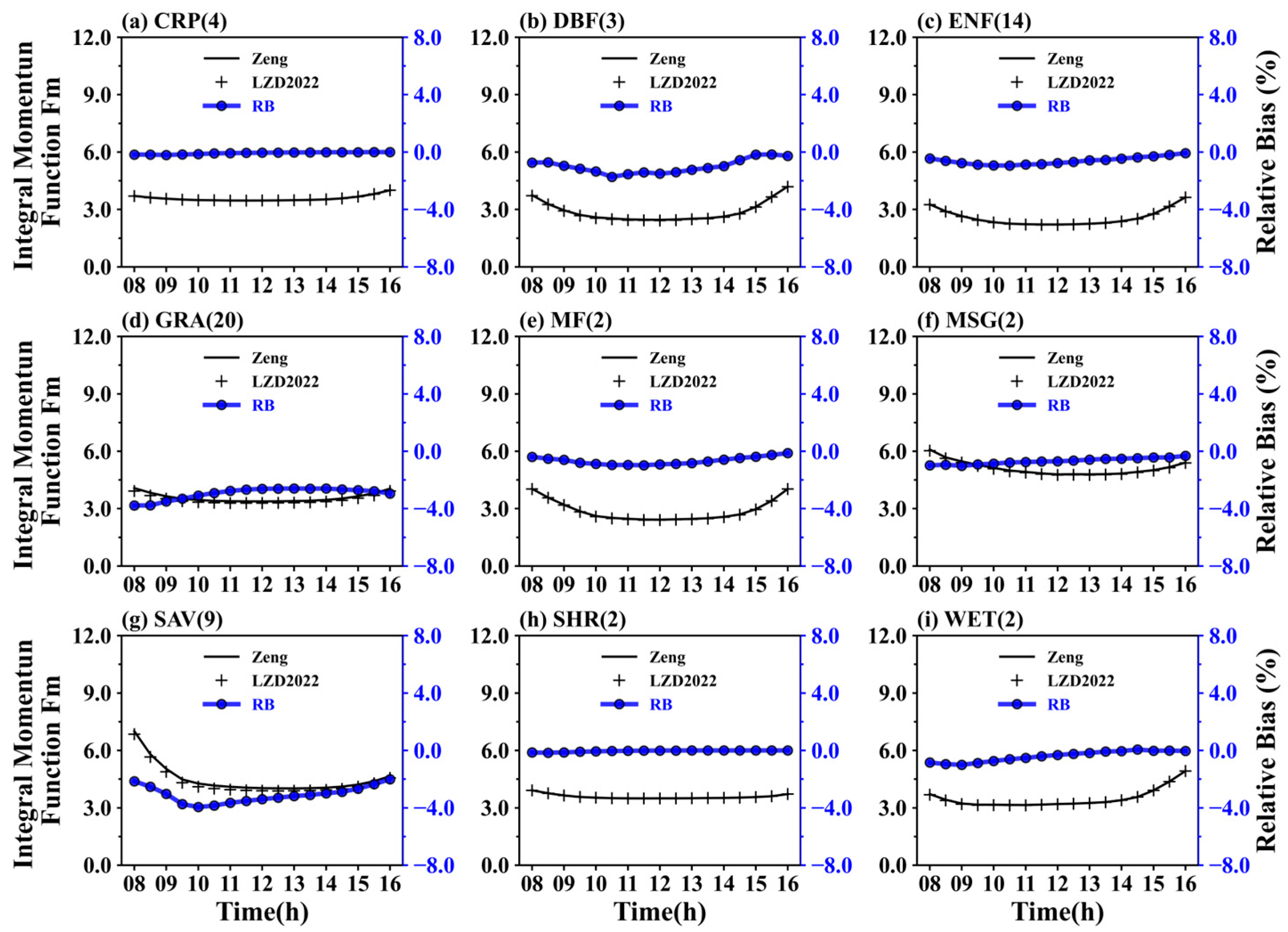
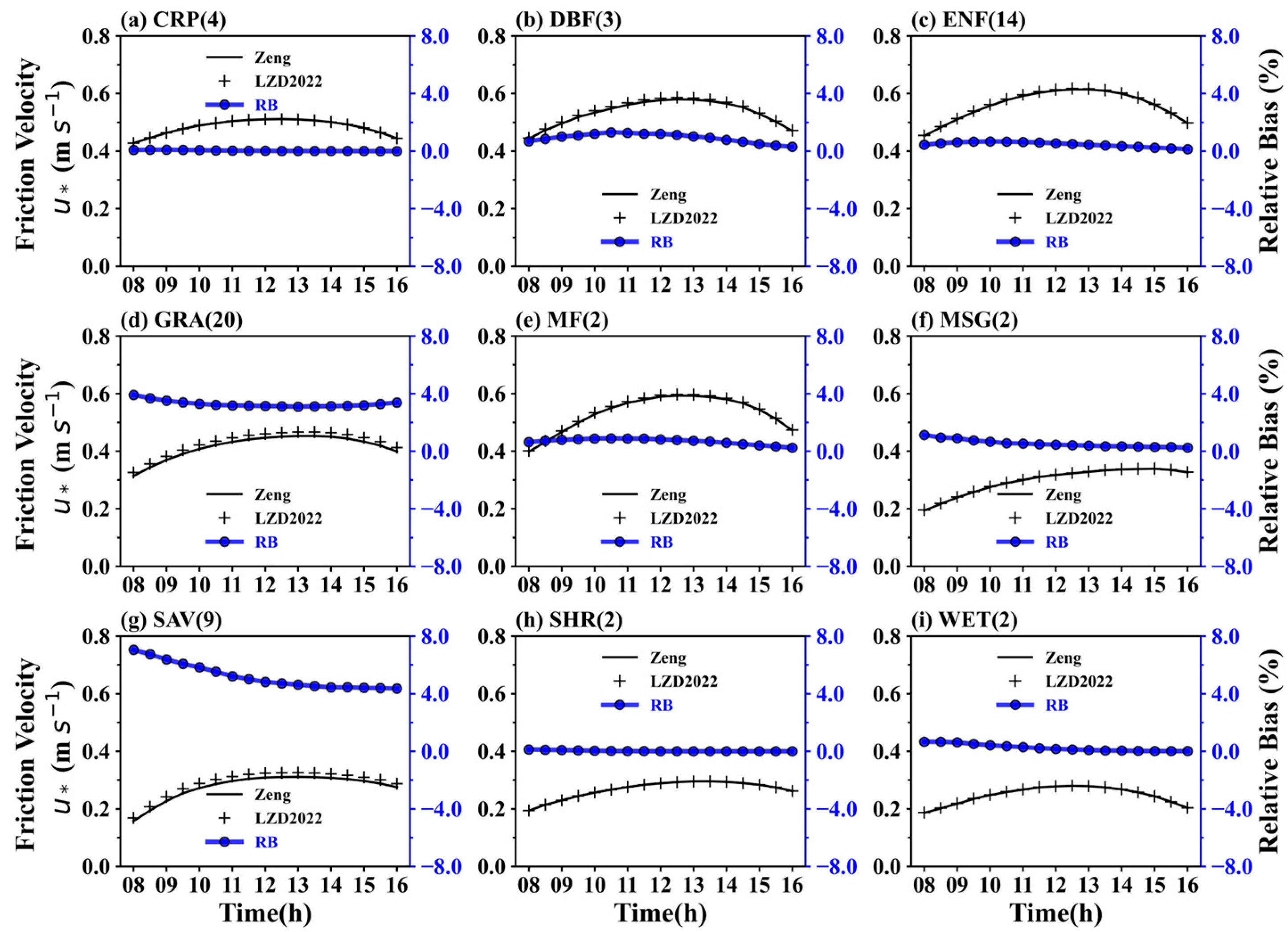
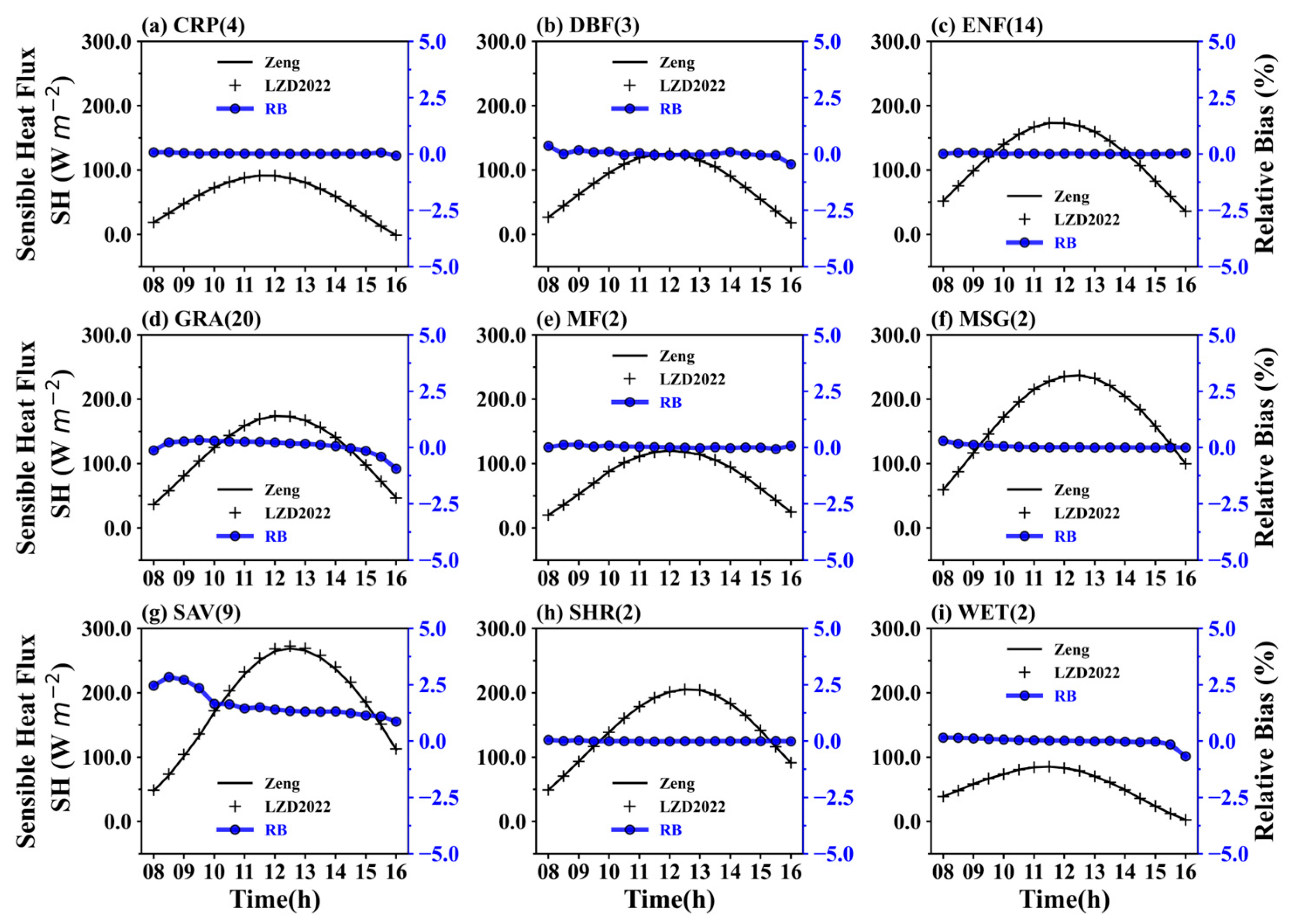
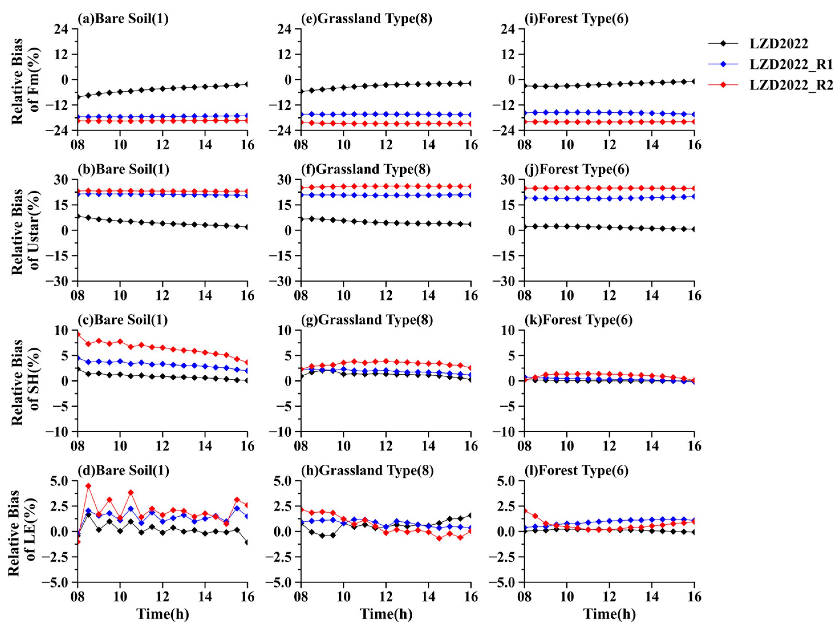
3.1. Comparison of Modified and Classical Flux-Gradient Relations

This study first compares the simulation results of four variables from the LZD2022 and the ZENG schemes: the integral momentum function (Fm), friction velocity ( u * ), sensible heat flux (SH), and latent heat flux (LE) across various land cover types. This paper focuses on periods of atmospheric instability during the day (0800 LST–1600 LST).
Figure 2, Figure 3, Figure 4 and Figure 5 present the multi-year averages and relative biases of Fm, u * , SH, and LE for the LZD2022 and ZENG schemes across various land cover types. For most land cover types (e.g., DBF, ENF, MF, MSG, SHR, and WET), the simulation results of the LZD2022 and ZENG schemes were almost identical, with relative biases near 0%. For some land cover types (e.g., GRA and SAV), the simulation results showed minor variations. The integral momentum function (Fm) decreased by a relative bias between 2% and 4%. The friction velocity ( u * ) increased by a relative bias between 3% and 8%. Additionally, the variations in sensible heat flux (SH) and latent heat flux (LE) were smaller compared to friction velocity, with relative biases of less than 3% for SH and less than 1.5% for LE.
Overall, the differences between LZD2022 and ZENG were little, particularly in heat flux. Further analysis will investigate the causes of these minor differences. By examining the mechanisms of surface flux parameterization, we aimed to identify the key factors that influence the performance of these schemes.

3.2. Factors Contributing to Minor Differences

The integral momentum function Fm (Equation (A6)) can also be written as:
Fm = 0 ζ ϕ m ( ζ ) ζ d ζ
The differences between the LZD2022 scheme and the ZENG scheme arise from 0 ζ ϕ m ( ζ ) ζ d ζ in Equation (7), which represents the integral of ϕ m ( ζ ) ζ with respect to ζ over the range from 0 to ζ .
To facilitate analysis, we define the integral of ϕ m ( ζ ) ζ over the range from 0 to ζ in the ZENG scheme as Fm ZENG , and the corresponding integral of ϕ m ( ζ ) ζ in the same interval for LZD2022 as Fm LZD 2022 . In Equation (5), the dimensionless wind speed gradient in LZD2022 consists of two terms. Specifically, ϕ m 1 ( ζ ) has the same form as in ZENG, while ϕ m 3 ( ζ ) represents a new term. Figure A1 in Appendix A shows a schematic diagram of Fm A 1 , Fm A 2 , and Fm A 3 . In this study, we define Fm A 1 = 0 ζ ϕ m 1 ( ζ ) ζ d ζ as the component that overlaps with ZENG in LZD2022, with ζ ranging from ζ = 0 to a transition value of ζ (denoted as ζ m 2 ). Similarly, we define Fm A 2 = ζ m 2 ζ ϕ m 3 ( ζ ) ζ d ζ as a new term that accounts for the effects of large eddies for ζ < ζ m 2 . Additionally, Fm A 3 represents the difference between the integrals of ZENG and LZD2022, which allows us to assess the discrepancies between the two schemes. The integral in LZD2022, denoted as Fm LZD 2022 , is the sum of Fm A 1 and Fm A 2 . The integral in ZENG (denoted Fm ZENG ) is the sum of Fm A 1 , Fm A 2 , and Fm A 3 . The exact forms of Fm A 1 and Fm A 2 under unstable conditions are
Fm A 1 = ln z z 0 m ψ m 1 ( ζ ) + ψ m ( z 0 m L ) , Fm A 2 = 0 for   ζ m 2 < ζ < 0 Fm A 1 = ln ζ m 2 L z 0 m ψ m ( ζ m 2 ) + ψ m ( z 0 m L ) , Fm A 2 = 2 B m 2 ( ζ ) 1 / 2 ( ζ m 2 ) 1 / 2 for   ζ < ζ m 2
In this study, Fm A 1 / ( Fm A 1 + Fm A 2 ) denotes the ratio of the overlapping component in the LZD2022 scheme with ZENG. Figure 6 shows the probability of overlapping distribution for different land cover types in LZD2022. As shown in Figure 6, for all land cover types, the ratio Fm A 1 / ( Fm A 1 + Fm A 2 ) mostly fell within the range of 0.7 to 1.0, with the highest proportion in the 0.9–1.0 range. For CRP, GRA, SHR, and WET, the proportion in the 0.9–1.0 range exceeded 90%. For MSG and SAV, the proportion in the 0.8–1.0 range exceeded 80%. For forest-type sites, such as DBF, ENF, and MF, the proportion in the 0.7–1.0 range exceeded 80%. Table 2 presents the average proportion of Fm A 1 relative to ( Fm A 1 + Fm A 2 ) . For all land cover types, the ratio of Fm A 1 to ( Fm A 1 + Fm A 2 ) exceeded 85%, with seven land cover types (i.e., CRP, ENF, GRA, MSG, SAV, SHR, and WET) showing Fm A 1 proportions greater than 90%. This suggests a significant overlap between LZD2022 and ZENG, resulting in minor differences between the two schemes.

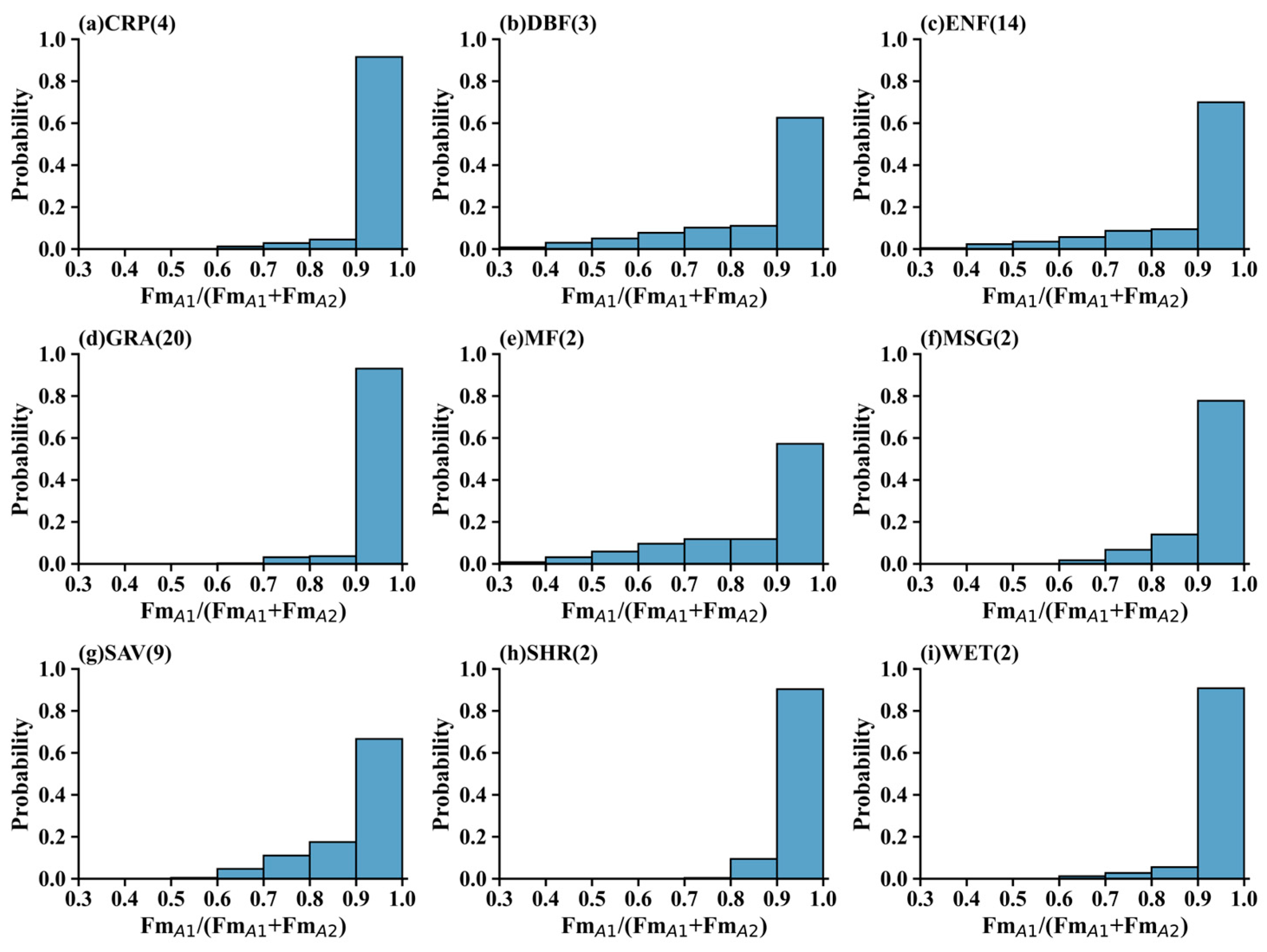
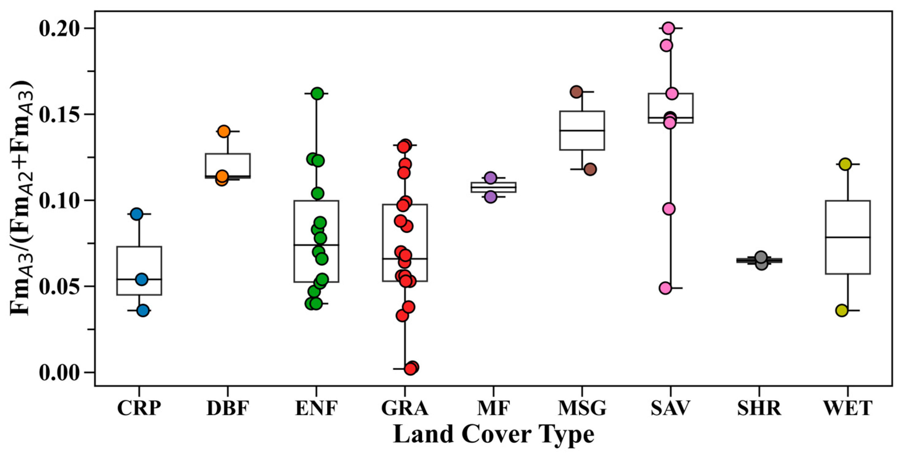
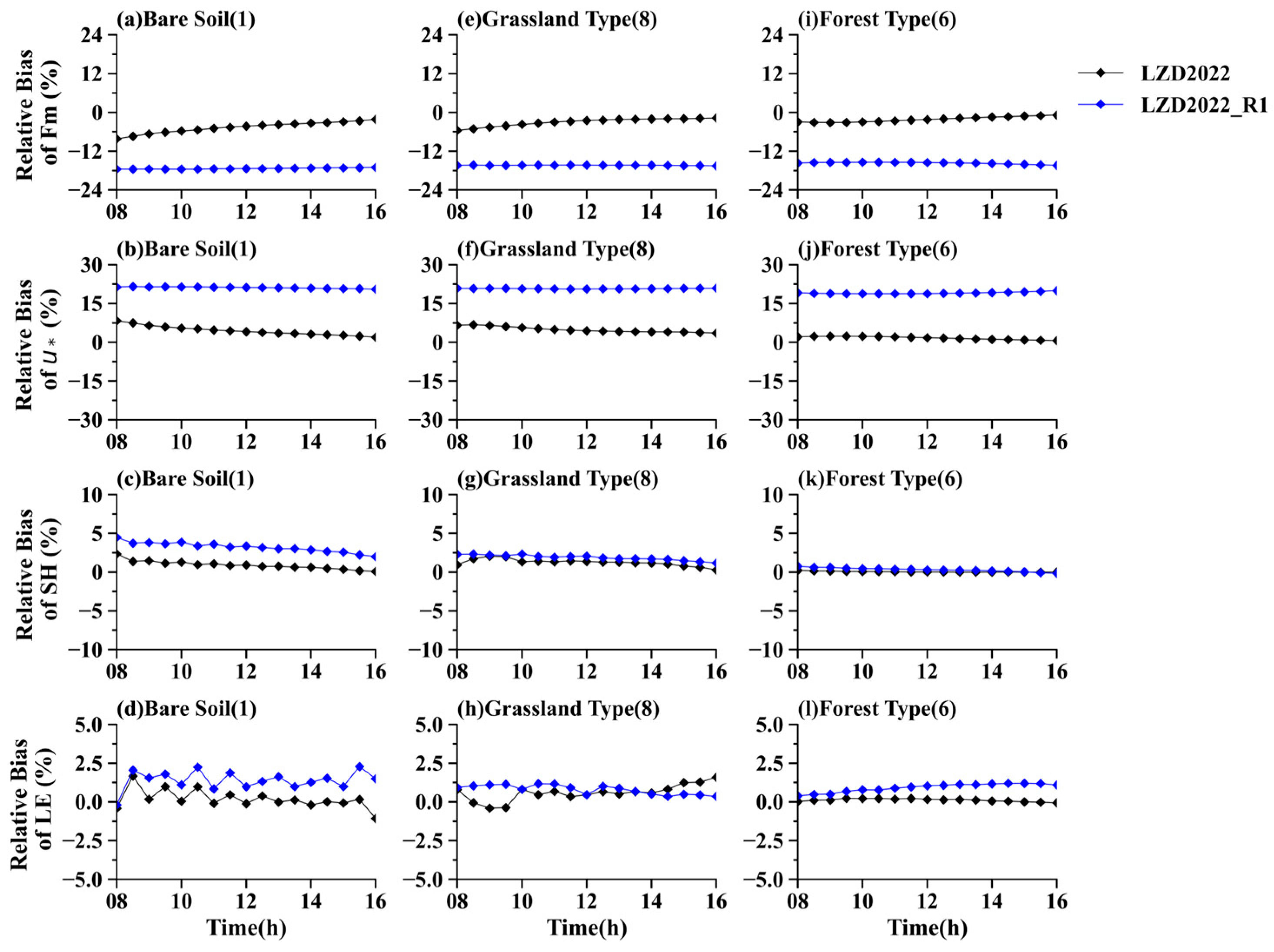
3.3. Overlapping Contributions and Indirect Influences

Section 3.2 shows that a rigorous comparison between LZD2022 and ZENG requires removing the overlapping contributions in LZD2022, quantified as Fm A 1 . By excluding Fm A 1 , Fm LZD 2022 consists solely of Fm A 2 , while Fm ZENG includes both Fm A 2 and Fm A 3 . Thus, Fm A 3 corresponds to the difference between Fm LZD 2022 and Fm ZENG . In this study, we introduced a parameter α , defined as α = Fm A 3 / ( Fm A 2 + Fm A 3 ) , to quantify the proportion of differences between the LZD2022 and ZENG schemes relative to the ZENG scheme, after excluding overlapping components. A larger α value indicates that the differences between the two schemes are significant. Subsequently, Fm = ( 1 α ) Fm ZENG represents Fm LZD 2022 after removing the overlapping contributions.
Figure 7 presents the distribution of α , denoted by Fm A 3 / ( Fm A 2 + Fm A 3 ) across nine land cover types. The α values did not exhibit any clear pattern among the different land cover types, ranging from 0.01 to 0.2. This indicates that, even after removing the overlapping contributions, the differences between the LZD2022 and ZENG schemes constituted a relatively small ratio within the ZENG scheme, with a maximum value of 0.2. Notably, the highest ratio was observed at the US-Ton site with the SAV land cover type.
In this study, we set the Fm value to ( 1 α ) Fm ZENG to represent the LZD2022 scheme after removing the overlapping contributions (hereafter referred to as LZD2022_R1). The α value used here was 0.2, taken from the US-Ton site as a reference. Figure 8 compares the relative biases of the LZD2022 and LZD2022_R1 relative to ZENG across bare soil, grassland-type, and forest-type sites. Due to the absence of bare soil observation sites in the FLUXNET2015 database, we set the US-Ton site as a bare soil site in this study. Furthermore, we selected eight grassland-type sites (i.e., AU-DaS, AU-Dry, AU-Lit, CA-SF3, CN-Du2, DE-Geb, IT-Amp, and US-Ton) and six forest-type sites (i.e., CH-Dav, DE-Tha, IT-Isp, RU-Fyo, US-Me2, and US-Me4) for detailed analysis. As shown in Figure 8, the relative bias in the LZD2022_R1 scheme was greater than that in the LZD2022 scheme for each land cover type. Taking the friction velocity u * as an example (Figure 8b,f,j), the relative bias between the LZD2022 and ZENG schemes was generally less than 8%, whereas the relative bias between the LZD2022_R1 and ZENG schemes ranged from 15% to 22%. This suggests that after eliminating the overlapping contributions, the LZD2022_R1 scheme exhibited more significant changes compared to the LZD2022 scheme. This result emphasizes the importance of considering overlapping effects in model comparisons, suggesting that researchers should fully recognize the potential impact of overlapping components when conducting scheme evaluations. Furthermore, across all land cover types, the relative bias of sensible heat flux (SH) and latent heat flux (LE) remained consistently smaller than that of friction velocity ( u * ), even after removing the effects of overlapping components. In the LZD2022_R1 scheme, specifically, the relative bias of friction velocity was approximately 22%, while the relative biases of both sensible heat flux and latent heat flux were less than 5%. This indicates that the response of friction velocity to large eddies was more pronounced compared to that of heat flux. Additionally, the simulation performance of each variable varied across different land cover types. For the integral momentum function (Fm) and friction velocity ( u * ) (as shown in Figure 8a,b,e,f,i,j), the simulation differences between the LZD2022 and LZD2022_R1 scheme were similar across the three land cover types. This suggests that the response of momentum flux to large eddies was relatively consistent across different land cover types. In contrast, for the sensible heat flux (SH) (Figure 8c,g,k), the differences between the LZD2022 and LZD2022_R1 scheme were most pronounced at bare soil sites, followed by grassland-type sites, with the smallest differences observed at forest-type sites. This indicates that, for sensible heat flux, the response to large eddies was most significant at bare soil sites, followed by grassland-type sites, and least at forest-type sites. Similarly, for latent heat flux (LE) (Figure 8d,h,l), the relative bias between the LZD2022 and LZD2022_R1 scheme was most prominent at bare soil sites, moderately pronounced at forest-type sites, and minimal at grassland-type sites.
Based on the above analysis, after removing the overlapping effects of the ZENG scheme, the variations in heat flux were minimal, particularly at grassland-type and forest-type sites. In practical applications, surface flux parameterization is an iterative process. As discussed in Section 3.1, due to the influence of large eddies, the decreases in integral momentum function (Fm) leads to an increase in the surface friction velocity ( u * ), which in turn causes an increase in the Obukhov length L (Equation (A5)) and a decrease in stability parameter( ζ = z / L ), ultimately approaching a neutral condition. According to the empirical expression for the dimensionless temperature gradient (Equation (2)), ϕ h ( ζ ) increases, which ultimately leads to a decrease in the dimensionless temperature scale θ * (Equation (A4)). Since the changes in u * and θ * are opposite, the variations in sensible heat flux remain insignificant (Equation (A2)). Overall, under the influence of large eddies, friction velocity ( u * ) influences the stability, which, in turn, affects the dimensionless temperature scale ( θ * ). Consequently, this indirect influence mitigates the impact of large eddies on heat flux.
To mitigate the indirect influence of large eddies on heat flux, we developed the LZD2022_R2 scheme. Specifically, LZD2022_R2 builds on LZD2022_R1 by further blocking the indirect effects of large eddies on heat flux. Figure 9 shows the relative biases of integral momentum function (Fm), friction velocity ( u * ), sensible heat flux (SH), and latent heat flux (LE) under the LZD2022, LZD2022_R1, and LZD2022_R2 schemes across three land cover types. The results show that, after blocking the indirect influence on heat flux, the relative change in sensible heat flux (SH) increased across all three surface types (Figure 9c,g,k), with the most pronounced change occurring at bare soil sites, followed by grassland-type sites, and the least at forest-type sites. Specifically, comparing the changes in sensible heat flux (SH) between the LZD2022_R1 and LZD2022_R2 schemes relative to ZENG, the relative bias at bare soil sites increased from 3% to approximately 8%, at grassland-type sites from 2% to around 4%, and at forest-type sites from little to about 2%. This finding indicates that different land cover types modulate the impact of large eddies in distinct ways. The response to large eddies was most pronounced at bare soil sites, followed by grassland sites, with the least response observed at forest sites. In contrast, for latent heat flux (LE), after removing the indirect influence on heat flux, the relative bias at bare soil sites increased (Figure 9d), while no clear pattern emerged at grassland and forest sites (Figure 9h,l). This suggests that the effect of large eddies on latent heat flux is more complex than its impact on sensible heat flux.

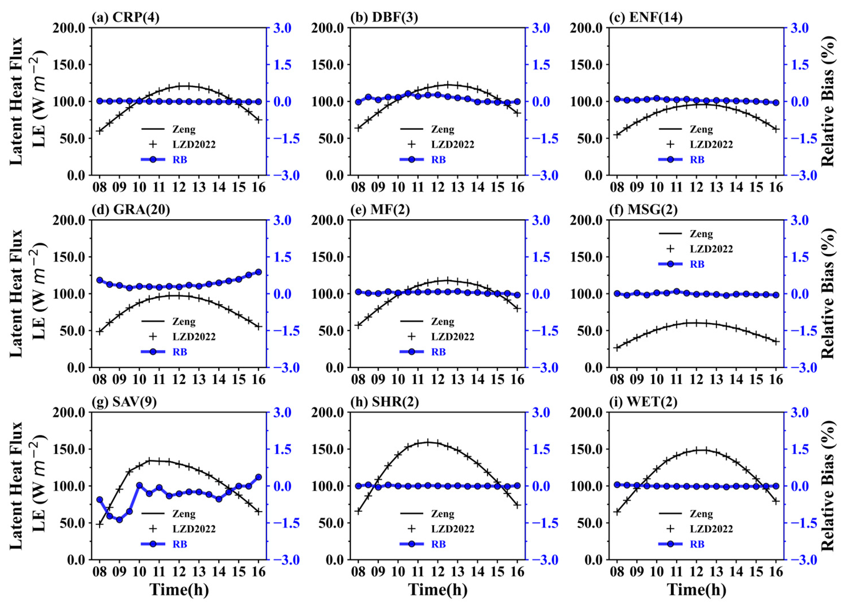
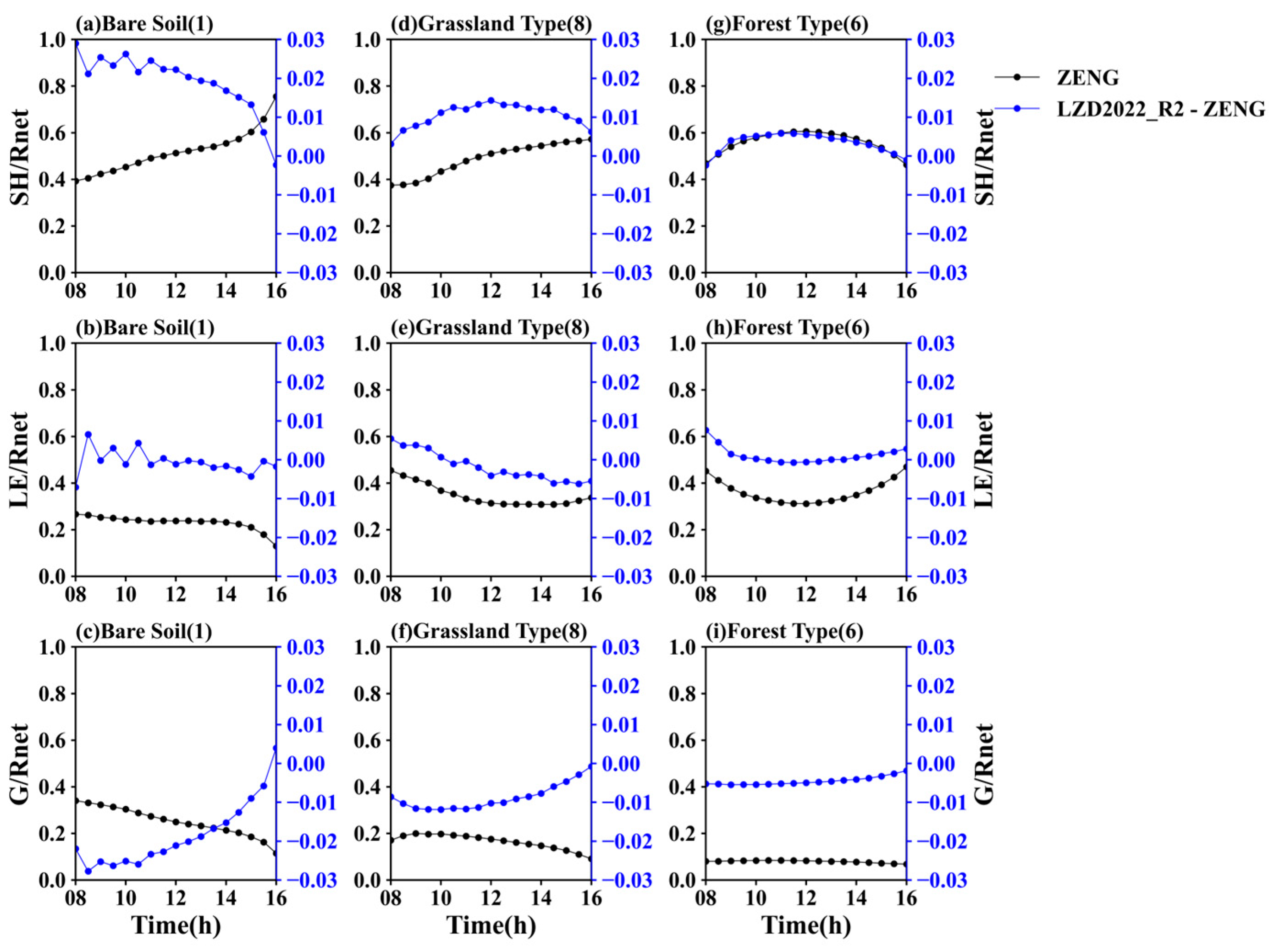
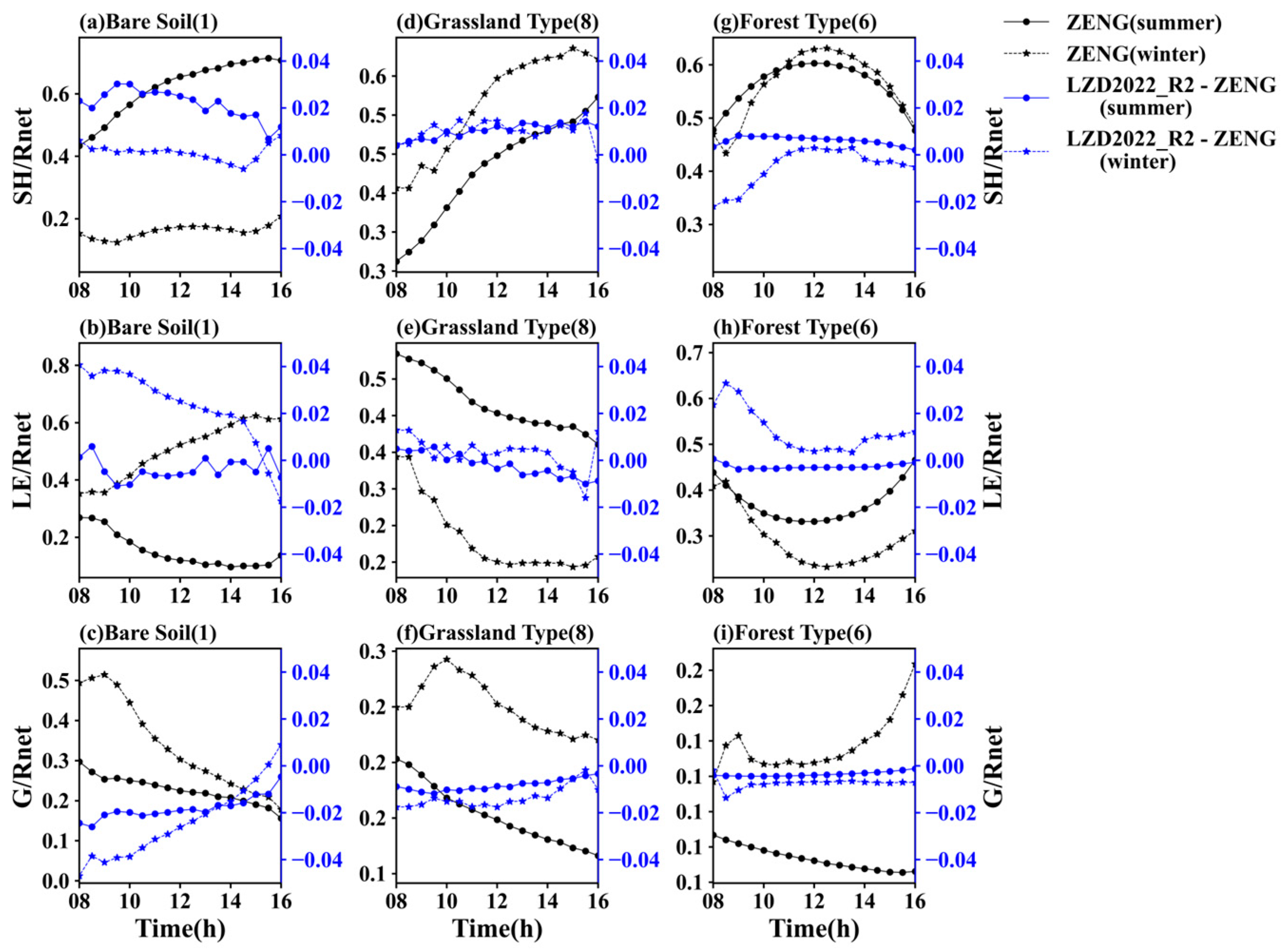
3.4. Surface Energy Balance

In this section, we explore the energy partitioning characteristics associated with different land surface types. Figure 10 illustrates the daily patterns of sensible heat flux (SH), latent heat flux (LE), and ground heat flux (G) relative to net radiation (Rnet) for three surface types: bare soil, grassland-type, and forest-type sites. It is evident that, on bare soil, the SH/Rnet ratio rose sharply during the afternoon, which implies a constrained evaporative process that favors sensible heat release. Meanwhile, grassland-type and forest-type sites exhibited more uniform SH/Rnet profiles, suggesting enhanced transpiration and moisture control. Moreover, the latent heat contribution (LE/Rnet) was lower in bare soil compared to the other two surface types, suggesting that vegetation facilitated greater conversion of net radiation into latent heat. The G/Rnet values were uniformly low, especially for grassland and forest. The figure also shows the difference in energy partitioning between the LZD2022_R2 and ZENG schemes. Notably, differences in SH/Rnet and G/Rnet were most significant for bare soil, followed by grassland-type sites, and were least apparent in forest-type sites. For LE/Rnet, the differences remained largely uniform across all surfaces. Collectively, these results indicate that the large eddy effects induced more substantial energy partitioning changes on bare soil, moderate changes on grassland-type, and minimal effects on forest-type sites, likely due to varying vegetation cover, soil moisture conditions, and transpiration dynamics.
Figure 11 presents the diurnal variations in the ratios of sensible heat flux (SH), latent heat flux (LE), and soil heat flux (G) to net radiation (Rnet) for different land types (bare soil, grassland-type, forest-type sites) during the summer and winter periods. Firstly, Figure 11 presents the seasonal differences in energy partitioning for the ZENG scheme, with black circles and star symbols marking the data for summer and winter. The results indicate a significant seasonal contrast, especially in bare soil where the variation was greatest, followed by grassland and then forest. Furthermore, Figure 11 illustrates the seasonal differences in energy partitioning between the ZENG and LZD2022_R2 schemes, as indicated by blue circles and star symbols. On bare soil, the differences in energy partitioning between the ZENG and LZD2022_R2 schemes were more pronounced for SH/Rnet in summer and for LE/Rnet in winter. In contrast, on grassland-type surfaces, the differences between the two schemes were relatively consistent between summer and winter. For forest-type surfaces, the difference in LE/Rnet in winter was particularly significant.

4. Conclusions and Discussion

This study employed the Common Land Model (CoLM2014) along with FLUXNET2015 and ERA5 data to evaluate the modified flux-gradient relations, which account for large eddy effects under unstable conditions, as outlined in the LZD2022 scheme introduced by [24]. The aim was to test its applicability in improving the accuracy of surface flux parameterization compared to classical schemes. First, we conducted a comparative analysis between the LZD2022 scheme and the widely used surface flux parameterization scheme [31]. Subsequently, we investigated the underlying physical mechanisms governing the flux-gradient relations and identified the key factors influencing surface flux parameterization through model simulations. Finally, we assessed the effects of large eddies on different land cover types, including bare soil, grassland-type, and forest-type sites, and explored their energy distribution patterns.
While preliminary comparisons indicated minimal differences between the LZD2022 scheme and the ZENG scheme, subsequent analysis demonstrated that two distinct factors contributed significantly to this result. The first significant factor is attributed to the LZD2022 scheme’s implementation of a Dyer-form dimensionless wind speed gradient [5], which ensures continuity of the wind profile under near-neutral conditions and overlaps with the gradient employed in the ZENG scheme. As a result, more than 85% of the dimensionless wind speed gradient is shared between the two schemes, leading to little differences. Therefore, to accurately evaluate the potential effects of large eddies on surface fluxes, it is crucial to remove the overlapping contribution in the LZD2022 scheme. After eliminating the overlap between the LZD2022 and ZENG schemes, significant differences in friction velocity ( u * ) were observed, with these differences becoming more pronounced. However, the changes in sensible heat flux (SH) and latent heat flux (LE) were relatively small. Further analysis indicates that a crucial second factor is the role of friction velocity in affecting atmospheric stability, which subsequently governs the dimensionless temperature scale ( θ * ) and reduces the effect of large-scale eddies on heat flux. After blocking the indirect influence on heat flux, the variations in sensible heat flux (SH) became significantly more pronounced, highlighting the stronger response of heat flux to large eddies. Considering the two factors discussed above, our research advises that, under near-neutral conditions, an alternative form of the dimensionless gradient formulation be adopted in the LZD2022 scheme to account for large eddy effects. In addition, we recommend that the model application of LZD2022 remove the indirect impact on stability, which mitigates the influence of large eddies on heat flux.
This study compared the impact of large eddies across three different surface types: bare soil, grassland-type, and forest-type sites. The results show that the response of momentum flux to large eddies is relatively consistent across different land cover types. In contrast, the response of sensible heat flux to large eddies was most pronounced at bare soil sites, followed by grassland-type sites, with the least effect at forest-type sites. For latent heat flux (LE), the influence of large eddies was most pronounced at bare soil sites, showing a response similar to that of sensible heat flux. However, the latent heat flux response to large eddies at grassland-type and forest-type sites was inconsistent, indicating that the mechanisms governing latent heat flux are more complex than those influencing sensible heat flux. Furthermore, our analysis of energy partitioning revealed that large eddy effects induce more pronounced changes on bare soil, moderate changes on grassland-type surfaces, and minimal effects on forest, likely due to differences in vegetation cover, soil moisture conditions, and transpiration dynamics. These findings indicate that different land cover types respond differently to the influence of large eddies.
This study employed an offline land surface model to evaluate a scheme that considers the effects of large eddies. Through an in-depth analysis of the surface flux parameterization mechanisms, this study provides recommendations for improving the scheme that accounts for large eddy effects. Additionally, by comparing the response of surface fluxes and energy partitioning across different land cover types, this work has contributed to enhancing our understanding of land–atmosphere interactions.

Author Contributions

Conceptualization, H.H. and S.L.; methodology, H.H. and S.L.; software, H.H.; validation, H.H.; formal analysis, H.H. and S.L.; investigation, H.H. and S.L.; resources, S.L.; data curation, H.H.; writing—original draft preparation, H.H.; writing—review and editing, H.H., L.L., Q.S. and S.L.; visualization, H.H.; supervision, S.L.; project administration, S.L.; funding acquisition, S.L. All authors have read and agreed to the published version of the manuscript.

Funding

This research was funded by the Natural Science Foundation of China (under grant 42375163).

Institutional Review Board Statement

Not applicable.

Informed Consent Statement

Not applicable.

Data Availability Statement

The observation site information used in this study can be downloaded from FLUXNET (https://fluxnet.org/data/fluxnet2015-dataset/, accessed 6 March 2021). The boundary layer height data can be downloaded from ERA5 (https://www.ecmwf.int/en/forecasts, accessed 12 March 2025).

Acknowledgments

The Editor and reviewers are thanked for constructive comments. We thank the Editor and reviewers for their valuable comments.

Conflicts of Interest

Informed consent was obtained from all subjects involved in this study.

Abbreviations

The following abbreviations are used in this manuscript:
ZENGClassical flux-gradient relations scheme under unstable conditions.
LZD2022Modified flux-gradient relations scheme under unstable conditions.
LZD2022_R1Derived from the LZD2022 scheme after eliminating the overlapping effects of the ZENG scheme.
LZD2022_R2Derived from the LZD2022_R1 scheme by blocking the indirect influence on heat flux.
Fm ZENG 
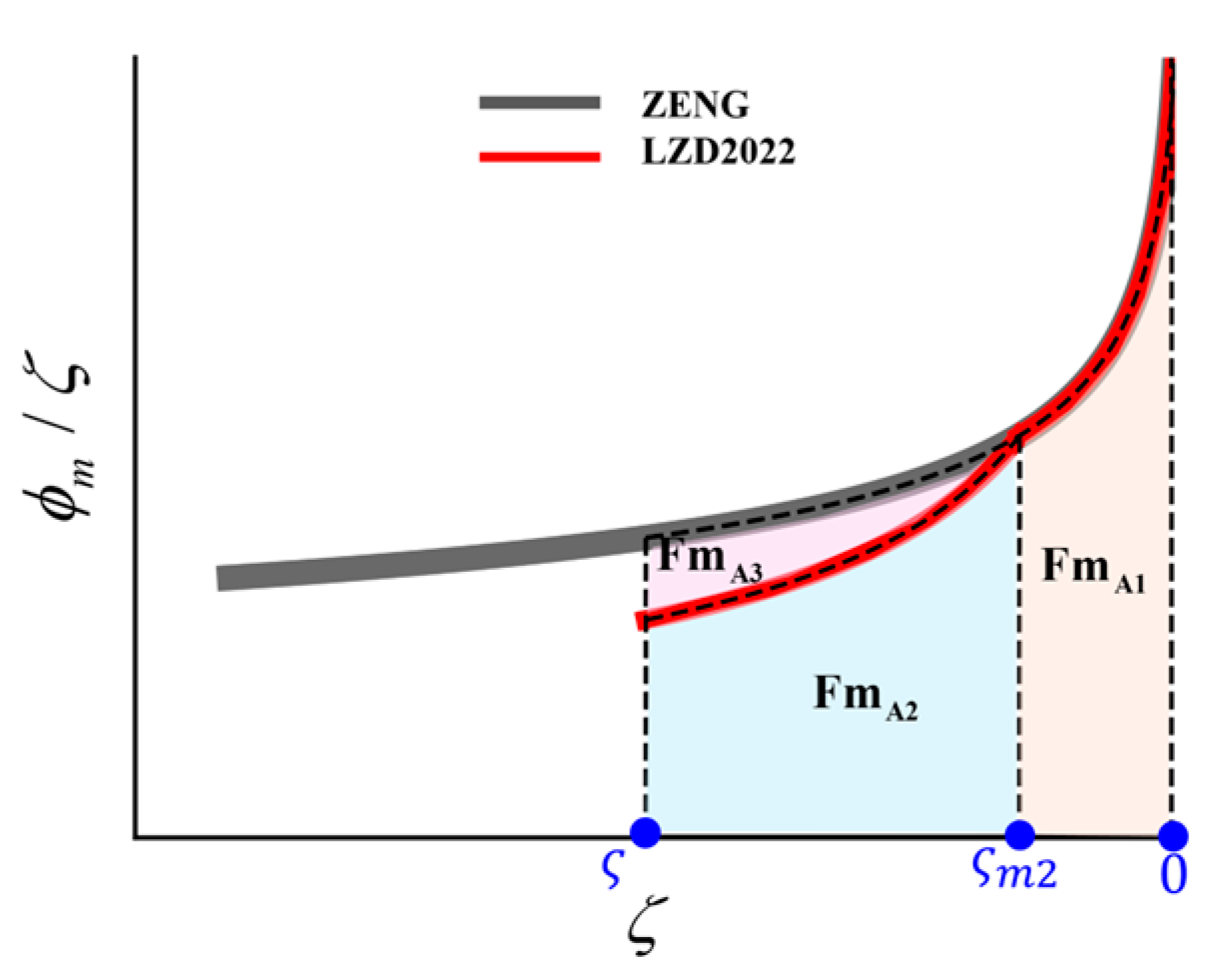
Integral momentum function in ZENG scheme.
Fm LZD 2022 Integral momentum function in LZD2022 scheme.
Fm A 1 The overlapping component with ZENG in LZD2022 scheme.
Fm A 2 The term accounting large eddy effects in LZD2022 scheme.
Fm A 3 Difference between ZENG and LZD2022 scheme.

Appendix A

Appendix A.1

Surface fluxes of momentum flux ( τ ) and heat flux ( H ) are defined as follows:
τ = ρ u * 2
H = ρ c p u * θ *
where ρ is air density, c p is specific heat capacity under constant pressure, u * is the dimensionless velocity scale (i.e., friction velocity), and θ * is the dimensionless temperature scale.
Following the Monin–Obukhov similarity theory, the scaling variables u * and θ * in surface fluxes can be obtained from flux-gradient relations, which are expressed as:
κ z u * U z = ϕ m ( ζ )
κ z θ * Θ z = ϕ h ( ζ )
where z is the reference height, κ is the Kármán constant, U and Θ are the mean wind speed and temperature, ζ = z / L is the stability parameter, and L is the Obukhov length, defined as:
L = u * 3 Θ 0 κ g ( w θ ) 0 ¯
where Θ 0 is the near-surface temperature, ( w θ ) 0 ¯ is the near-surface kinematic heat flux, and g is the gravitational acceleration.
Integration of Equations (A3) and (A4) from the height above ground can be written as:
U z = u * κ Fm
Θ z Θ s = θ * κ Fh
where Fm = ln z z 0 m ψ m ( ζ ) refers to the integral of the profile function for momentum, and Fh = ln z z 0 h ψ h ( ζ ) is the integral of the profile function for temperature. z 0 m and z 0 h are the roughness lengths for momentum and heat, respectively. Θ s is the surface skin temperature. ψ m and ψ h are the stability functions for momentum and heat, respectively. The specific expressions of ψ m and ψ h can be found in [29]. For a comprehensive understanding of the derivation and application of this formula, refer to the detailed discussion provided in that article.

Appendix A.2

Figure A1. Schematic diagram of Fm A 1 , Fm A 2 , and Fm A 3 . ζ m 2 is the intersection of the ZENG scheme and the LZD2022 scheme. Fm A 1 , Fm A 2 , and Fm A 3 are the integral areas of ϕ m ( ζ ) / ζ over ζ , respectively.
Atmosphere 16 00328 g0a1

References

  1. Dai, Y.; Williams, I.N.; Qiu, S. Simulating the effects of surface energy partitioning on convective organization: Case study and observations in the US Southern Great Plains. J. Geophys. Res. Atmos. 2021, 126, e2020JD033821. [Google Scholar] [CrossRef]
  2. Dai, Y.; Williams, I.N. Land surface effects on shear balance of squall lines. J. Geophys. Res. Atmos. 2022, 127, e2021JD035436. [Google Scholar] [CrossRef]
  3. Monin, A.S.; Obukhov, A.M. Basic Laws of Turbulent Mixing in the Atmospheric Surface Layer. Contrib. Geophys. Inst. Slovak Acad. Sci. 1954, 51, e187. [Google Scholar]
  4. Businger, J.A.; Wyngaard, J.C.; Izumi, Y.; Bradley, E.F. Flux-profile relationships in the atmospheric surface layer. J. Atmos. Sci. 1971, 28, 181–189. [Google Scholar] [CrossRef]
  5. Dyer, A.J. A Review of Flux-Profile Relationships. Bound.-Layer Meteorol. 1974, 7, 363–372. [Google Scholar] [CrossRef]
  6. Hogstrom, U. Non-dimensional Wind and Temperature Profiles in the Atmospheric Surface Layer: A Re-Evaluation. Bound.-Layer Meteorol. 1988, 42, 55–78. [Google Scholar] [CrossRef]
  7. Hogstrom, U. Review of Some Basic Characteristics of the Atmospheric Surface Layer. Bound.-Layer Meteorol. 1996, 78, 215–246. [Google Scholar] [CrossRef]
  8. Panofsky, H.A.; Tennekes, H.; Lenschow, D.H.; Wyngaard, J.C. The Characteristics of Turbulent Velocity Components in the Surface Layer under Convective Conditions. Bound.-Layer Meteorol. 1977, 11, 355–361. [Google Scholar] [CrossRef]
  9. Khanna, S.; Brasseur, J.G. Analysis of Monin–Obukhov similarity from large-eddy simulation. J. Fluid Mech. 1997, 345, 251–286. [Google Scholar] [CrossRef]
  10. Katul, G.G.; Konings, A.G.; Porporato, A. Mean Velocity Profile in a Sheared and Thermally Stratified Atmospheric Boundary Layer. Phys. Rev. Lett. 2011, 107, 268502. [Google Scholar] [CrossRef]
  11. Banerjee, T.; Li, D.; Juang, J.-Y.; Katul, G. A Spectral Budget Model for the Longitudinal Turbulent Velocity in the Stable Atmospheric Surface Layer. J. Atmos. Sci. 2016, 73, 145–166. [Google Scholar] [CrossRef]
  12. Li, Q.; Gentine, P.; Mellado, J.P.; McColl, K.A. Implications of Nonlocal Transport and Conditionally Averaged Statistics on Monin–Obukhov Similarity Theory and Townsend’s Attached Eddy Hypothesis. J. Atmos. Sci. 2018, 75, 3403–3431. [Google Scholar] [CrossRef]
  13. Salesky, S.T.; Chamecki, M. Random Errors in Turbulence Measurements in the Atmospheric Surface Layer: Implications for Monin–Obukhov Similarity Theory. J. Atmos. Sci. 2012, 69, 3700–3714. [Google Scholar] [CrossRef]
  14. Deardorff, J.W. Numerical Investigation of Neutral and Unstable Planetary Boundary Layers. J. Atmos. Sci. 1972, 29, 91–115. [Google Scholar] [CrossRef]
  15. Kaimal, J.C.; Wyngaard, J.C.; Izumi, Y.; Coté, O.R. Spectral Characteristics of Surface-Layer Turbulence. Q. J. R. Meteorol. Soc. 1972, 98, 563–589. [Google Scholar] [CrossRef]
  16. Steeneveld, G.J.; Holtslag, A.A.M.; Debruin, H.A.R. Fluxes and Gradients in the Convective Surface Layer and the Possible Role of Boundary-Layer Depth and Entrainment Flux. Bound.-Layer Meteorol. 2005, 116, 237–252. [Google Scholar] [CrossRef]
  17. McNaughton, K.G. On the Kinetic Energy Budget of the Unstable Atmospheric Surface Layer. Bound.-Layer Meteorol. 2006, 118, 83–107. [Google Scholar] [CrossRef]
  18. Gioia, G.; Guttenberg, N.; Goldenfeld, N.; Chakraborty, P. Spectral Theory of the Turbulent Mean-Velocity Profile. Phys. Rev. Lett. 2010, 105, 184501. [Google Scholar] [CrossRef]
  19. Katul, G.G.; Li, D.; Chamecki, M.; Bou-Zeid, E. Mean Scalar Concentration Profile in a Sheared and Thermally Stratified Atmospheric Surface Layer. Phys. Rev. E 2013, 87, 023004. [Google Scholar] [CrossRef]
  20. Gao, Z.; Liu, H.; Russell, E.S.; Huang, J.; Foken, T.; Oncley, S.P. Large Eddies Modulating Flux Convergence and Divergence in a Disturbed Unstable Atmospheric Surface Layer. J. Geophys. Res. Atmos. 2016, 121, 1475–1492. [Google Scholar] [CrossRef]
  21. McColl, K.A.; Katul, G.G.; Gentine, P.; Entekhabi, D. Mean-Velocity Profile of Smooth Channel Flow Explained by a Cospectral Budget Model with Wall-Blockage. Phys. Fluids 2016, 28, 035107. [Google Scholar] [CrossRef]
  22. Mellado, J.P.; Van Heerwaarden, C.C.; Garcia, J.R. Near-Surface Effects of Free Atmosphere Stratification in Free Convection. Bound.-Layer Meteorol. 2016, 159, 69–95. [Google Scholar] [CrossRef]
  23. Cheng, Y.; Li, Q.; Li, D.; Gentine, P. Logarithmic Profile of Temperature in Sheared and Unstably Stratified Atmospheric Boundary Layers. Phys. Rev. Fluids 2021, 6, 034606. [Google Scholar] [CrossRef]
  24. Liu, S.; Zeng, X.; Dai, Y.; Yuan, H.; Wei, N.; Wei, Z.; Lu, X.; Zhang, S. A Surface Flux Estimation Scheme Accounting for Large-Eddy Effects for Land Surface Modeling. Geophys. Res. Lett. 2022, 49, e2022GL101754. [Google Scholar] [CrossRef]
  25. Bonan, G. A Land Surface Model (LSM Version 1.0) for Ecological, Hydrological, and Atmospheric Studies: Technical Description and User’s Guide; UCAR/NCAR: Boulder, CO, USA, 1996; 150p, NCAR/TN-417+STR. [Google Scholar]
  26. Dickinson, R.; Henderson-Sellers, A.; Kennedy, P. Biosphere-Atmosphere Transfer Scheme (BATS) Version 1e as Coupled to the NCAR Community Climate Model; UCAR/NCAR: Boulder, CO, USA, 1993; 72p, NCAR/TN-387+STR. [Google Scholar]
  27. Dai, Y.; Zeng, Q. A Land Surface Model (IAP94) for Climate Studies Part I: Formulation and Validation in off-Line Experiments. Adv. Atmos. Sci. 1997, 14, 433–460. [Google Scholar] [CrossRef]
  28. Yuan, H.; Dai, Y.; Xiao, Z.; Ji, D.; Shangguan, W. Reprocessing the MODIS Leaf Area Index Products for Land Surface and Climate Modelling. Remote Sens. Environ. 2011, 115, 1171–1187. [Google Scholar] [CrossRef]
  29. Shangguan, W.; Dai, Y.; Duan, Q.; Liu, B.; Yuan, H. A Global Soil Data Set for Earth System Modeling. J. Adv. Model. Earth Syst. 2014, 6, 249–263. [Google Scholar] [CrossRef]
  30. Dai, Y.; Dickinson, R.E.; Wang, Y.-P. A Two-Big-Leaf Model for Canopy Temperature, Photosynthesis, and Stomatal Conductance. J. Clim. 2004, 17, 2281–2299. [Google Scholar] [CrossRef]
  31. Zeng, X.; Zhao, M.; Dickinson, R.E. Intercomparison of Bulk Aerodynamic Algorithms for the Computation of Sea Surface Fluxes Using TOGA COARE and TAO Data. J. Clim. 1998, 11, 2628–2644. [Google Scholar] [CrossRef]
  32. Kader, B.A.; Yaglom, A.M. Mean Fields and Fluctuation Moments in Unstably Stratified Turbulent Boundary Layers. J. Fluid Mech. 1990, 212, 637–662. [Google Scholar] [CrossRef]
  33. Pastorello, G.; Trotta, C.; Canfora, E.; Chu, H.; Christianson, D.; Cheah, Y.-W.; Poindexter, C.; Chen, J.; Elbashandy, A.; Humphrey, M.; et al. The FLUXNET2015 Dataset and the ONEFlux Processing Pipeline for Eddy Covariance Data. Sci. Data 2020, 7, 225. [Google Scholar] [CrossRef] [PubMed]
  34. Baldocchi, D.; Falge, E.; Gu, L.; Olson, R.; Hollinger, D.; Running, S.; Anthoni, P.; Bernhofer, C.; Davis, K.; Evans, R.; et al. FLUXNET: A New Tool to Study the Temporal and Spatial Variability of Ecosystem-Scale Carbon Dioxide, Water Vapor, and Energy Flux Densities. Bull. Am. Meteorol. Soc. 2001, 82, 2415–2434. [Google Scholar] [CrossRef]
  35. Copernicus Climate Change Service (C3S). ERA5: Fifth Generation of ECMWF Atmospheric Reanalyses of the Global Climate. Copernicus Climate Change Service (C3S); European Centre for Medium: Reading, UK, 2017. [Google Scholar]
Figure 1. Geographical distribution of study sites classified according to the United States Geological Survey (USGS) ecosystem types. The color of each circle represents a specific ecosystem type according to the USGS classification. Numbers in parentheses indicate the number of sites within each USGS ecosystem group. A legend is provided for the color-coding of ecosystem types.
Atmosphere 16 00328 g001
Figure 2. Multi-year average diurnal variations of the integral momentum function (Fm) between ZENG (classical flux-gradient relation) and LZD2022 (modified flux-gradient relation) across different land cover types (0800 LST-1600 LST). The left y-axis represents the integral momentum function (Fm), while the right y-axis shows the relative bias of LZD2022 to ZENG for Fm. The analyzed land cover types include: (a) CRP, (b) DBF, (c) ENF, (d) GRA, (e) MF, (f) MSG, (g) SAV, (h) SHR, and (i) WET. Numbers in parentheses represent the number of sites per USGS classification group. In the figure, the solid black line represents the ZENG scheme, the black plus signs represent the LZD2022 scheme, and the blue solid line with circular markers represents the relative bias (%).
Atmosphere 16 00328 g002
Figure 3. Similar to Figure 2, but for friction velocity ( u * ).
Atmosphere 16 00328 g003
Figure 4. Similar to Figure 2, but for sensible heat flux (SH).
Atmosphere 16 00328 g004
Figure 5. Similar to Figure 2, but for latent heat flux (LE).
Atmosphere 16 00328 g005
Figure 6. Probability distribution of the overlapping component ratio in LZD2022 ( Fm A 1 / ( Fm A 1 + Fm A 2 ) ) for nine land cover types. The land cover types analyzed are (a) CRP, (b) DBF, (c) ENF, (d) GRA, (e) MF, (f) MSG, (g) SAV, (h) SHR, and (i) WET. Numbers in parentheses represent the number of sites within each United States Geological Survey (USGS) ecosystem group.
Atmosphere 16 00328 g006
Figure 7. Box plot showing the distribution of the ratio Fm A 3 / ( Fm A 2 + Fm A 3 ) across nine land cover types, where Fm A 3 / ( Fm A 2 + Fm A 3 ) represents the proportion of differences between the LZD2022 and ZENG schemes relative to the ZENG scheme after removing overlapping contributions. Each colored point corresponds to an individual site within its respective land cover type. The box represents the interquartile range, the line inside the box denotes the median, and the whiskers extend to the minimum and maximum values.
Atmosphere 16 00328 g007
Figure 8. Multi-year average diurnal variations of the relative bias for the LZD2022 (modified flux-gradient relation) and LZD2022_R1 scheme relative the ZENG (classical flux-gradient relation) scheme across bare soil, grassland-type, and forest-type sites. The LZD2022_R1 scheme represents the LZD2022 scheme after eliminating the overlapping effects of the ZENG scheme. This figure presents the following variables: integral momentum function (Fm), friction velocity ( u * ), sensible heat flux (SH), and latent heat flux (LE).
Atmosphere 16 00328 g008
Figure 9. Multi-year average diurnal variations of the relative bias for the LZD2022 (modified flux-gradient relation), LZD2022_R1, and LZD2022_R2 scheme relative to the ZENG (classical flux-gradient relation) scheme across bare soil, grassland-type, and forest-type sites. The LZD2022_R1 scheme represents the LZD2022 scheme after eliminating the overlapping effects of the ZENG scheme. The LZD2022_R2 scheme is derived from the LZD2022_R1 scheme by blocking the indirect influence on heat flux. This figure presents the following variables: integral momentum function (Fm), friction velocity ( u * ), sensible heat flux (SH), and latent heat flux (LE).
Atmosphere 16 00328 g009
Figure 10. Multi-year average diurnal variations in the ratios of sensible heat flux (SH), latent heat flux (LE), and soil heat flux (G) to net radiation (Rnet) for different land types (bare soil, grassland-type, forest-type sites). The left y-axis shows the energy flux contributions for the ZENG scheme, while the right y-axis displays the difference between the LZD2022_R2 and ZENG schemes.
Atmosphere 16 00328 g010
Figure 11. Multi-year average diurnal variations in the ratios of sensible heat flux (SH), latent heat flux (LE), and soil heat flux (G) to net radiation (Rnet) for different land types (bare soil, grassland-type, forest-type sites) during the summer and winter periods. The left y-axis shows the energy flux contributions for the ZENG scheme, while the right y-axis displays the difference between the LZD2022_R2 and ZENG schemes. Black solid circles represent the summer data for the ZENG scheme, and black star symbols represent the winter data for the ZENG scheme. Blue circles indicate the summer difference between the LZD2022_R2 and ZEN schemes, while blue star symbols show the winter difference.
Atmosphere 16 00328 g011
Table 1. Characteristics of FLUXNET Sites and Data Information.
Site NameLongitudeLatitudeYearLand Cover Type (USGS)Height (m)
AU-Cpr140.58−34.002011–2017Savanna20
AU-DaP131.32−14.062009–2012Grassland15
AU-DaS131.38−14.152010–2017Savanna23
AU-Dry132.37−15.252011–2015Savanna15
AU-How131.15−12.492003–2017Savanna23
AU-Lit130.79−13.12016–2017Savanna31
AU-Stp133.35−17.152010–2017Grassland4.8
BE-Bra4.5251.302004–2014Mixed Forest41.0
BE-Lon4.7450.552005–2014Irrigated Cropland and Pasture2.7
BE-Vie5.9950.301997–2014Mixed Forest40
CA-Qfo−74.3449.692004–2010Evergreen Needleleaf Forest24
CA-SF3−106.0054.092003–2005Mixed Shrubland/Grassland18.29
CH-Cha8.4147.212006–2014Grassland2
CH-Dav9.8546.811997–2014Evergreen Needleleaf Forest35
CN-Cng123.5044.592008–2009Grassland6
CN-Du2116.2842.042007–2008Grassland4
CN-HaM101.1837.372002–2003Grassland2.2
CZ-wet14.7749.022007–2014Herbaceous Wetland2.7
DE-Bay11.8650.141997–1999Evergreen Needleleaf Forest32
DE-Geb10.9151.102001–2014Irrigated Cropland and Pasture6
DE-Gri13.5150.942004–2014Grassland 3
DE-Hai10.4551.072000–2012Deciduous Broadleaf Forest42
DE-Kli13.5250.892005–2014Irrigated Cropland and Pasture3.5
DE-Obe13.7250.782008–2014Evergreen Needleleaf Forest30
DE-SfN11.3247.802013–2014Herbaceous Wetland6
DE-Tha13.5650.961998–2014Evergreen Needleleaf Forest42
DE-Wet11.4550.452002–2006Evergreen Needleleaf Forest30
DK-Lva12.0855.682005–2006Grassland2.5
DK-Sor11.6455.481997–2014Deciduous Broadleaf Forest57
ES-LMa−5.7739.942004–2006Savanna15.5
FI-Hyy24.29561.841996–2014Evergreen Needleleaf Forest23
FI-Sod26.6378367.362008–2014Evergreen Needleleaf Forest23
HU-Bug19.6046.692003–2006Grassland4
IE-Dri−8.7551.982003–2005Grassland10
IT-Amp13.6041.902003–2006Grassland4
IT-Isp8.6345.812013–2014Deciduous Broadleaf Forest38
IT-Noe8.1540.602004–2014Shrubland2
IT-SR210.2943.732013–2014Evergreen Needleleaf Forest22.5
NL-Ca14.9251.972003–2006Grassland20
NL-Loo5.7452.161997–2013Evergreen Needleleaf Forest24.4
RU-Fyo32.9256.462003–2014Evergreen Needleleaf Forest29
SD-Dem30.4713.282005–2009Savanna9
US-AR1−99.4236.422010–2012Grassland2.84
US-Aud−110.5031.592003–2005Grassland4
US-Bkg−96.8344.342005–2006Grassland4
US-Bo1−88.2940.001997–2006Irrigated Cropland and Pasture10
US-FPe−105.1048.302000–2006Grassland3.5
US-Goo−89.8734.252004–2006Grassland4
US-Ho1−68.7445.201996–2004Evergreen Needleleaf Forest30
US-KS2−80.671528.608582003–2006Shrubland3.5
US-Me2−121.55744.45232002–2014Evergreeen Needleleaf Forest32
US-Me4−121.6244.491996–2000Evergreeen Needleleaf Forest47
US-SRG−110.8231.782009–2014Grassland3.25
US-SRM−110.8631.822004–2014Savanna7.8
US-Ton−120.9638.432001–2014Savanna23.5
US-Var−120.9538.412001–2014Grassland2.2
US-Whs−110.0531.742008–2014Mixed Shrubland/Grassland6.5
US-Wkg−109.9431.732005–2014Grassland6.4
Table 2. Mean proportions of Fm A 1 / ( Fm A 1 + Fm A 2 ) across nine land cover types.
Land Cover Type
(USGS)
Fm A 1 / ( Fm A 1 + Fm A 2 )
CRP0.98
DBF0.88
ENF0.91
GRA0.98
MF0.87
MSG0.95
SAV0.92
SHR0.98
WET0.97
Disclaimer/Publisher’s Note: The statements, opinions and data contained in all publications are solely those of the individual author(s) and contributor(s) and not of MDPI and/or the editor(s). MDPI and/or the editor(s) disclaim responsibility for any injury to people or property resulting from any ideas, methods, instructions or products referred to in the content.

